Time-uniform, nonparametric, nonasymptotic confidence sequences

Steven R. Howard $^{1}$      Aaditya Ramdas $^{2,3}$      Jon McAuliffe $^{1,4}$      Jasjeet Sekhon $^{1,5}$

Departments of Statistics $^{1}$ and Political Science $^{5}$, UC Berkeley
Departments of Statistics and Data Science $^{2}$ and Machine Learning $^{3}$, Carnegie Mellon
The Voleon Group $^{4}$
{stevehoward,jonmcauliffe,sekhon}@berkeley.edu, [email protected]

August 9, 2022

Abstract

A confidence sequence is a sequence of confidence intervals that is uniformly valid over an unbounded time horizon. Our work develops confidence sequences whose widths go to zero, with nonasymptotic coverage guarantees under nonparametric conditions. We draw connections between the Cramér-Chernoff method for exponential concentration, the law of the iterated logarithm (LIL), and the sequential probability ratio test---our confidence sequences are time-uniform extensions of the first; provide tight, nonasymptotic characterizations of the second; and generalize the third to nonparametric settings, including sub-Gaussian and Bernstein conditions, self-normalized processes, and matrix martingales. We illustrate the generality of our proof techniques by deriving an empirical-Bernstein bound growing at a LIL rate, as well as a novel upper LIL for the maximum eigenvalue of a sum of random matrices. Finally, we apply our methods to covariance matrix estimation and to estimation of sample average treatment effect under the Neyman-Rubin potential outcomes model.

Executive Summary: In today's data-driven world, organizations routinely run sequential experiments like A/B tests to optimize online products and services. These tests generate data continuously as users interact, but traditional statistical methods treat the sample as fixed from the start. Peeking at results mid-experiment inflates the risk of false positives—declaring an effect real when it's not—often by a factor of two or more. This problem has grown urgent with the scale of modern experiments, where decisions must be timely and reliable, yet most analyses still ignore the sequential nature of the data.

This paper develops confidence sequences, a tool for building updating confidence intervals that remain valid no matter how long the experiment runs or when it stops. The goal is to create intervals that shrink toward the true value over time, under minimal assumptions about the data's distribution, ensuring at least 95% coverage (or whatever level is chosen) uniformly across all time points.

The authors use a high-level approach rooted in martingale theory—a way to track cumulative deviations in data streams—and connect it to classic ideas like exponential concentration bounds and the law of iterated logarithm. They focus on nonparametric settings, meaning no strong assumptions about data shape, and derive sequences for various cases, including bounded data, heavy-tailed distributions, matrix observations, and causal effects. Key tools include "stitching" linear bounds into curved ones over time epochs, mixture methods for exact boundaries, and self-normalization to estimate variance empirically. They test these on simulated data from independent observations over up to 100,000 points, comparing against fixed-sample and pointwise methods.

The core findings are fourfold. First, the methods yield intervals about twice as wide as standard fixed-sample ones but shrink at a rate of roughly the square root of (log log t over t), matching the theoretical limit from the law of iterated logarithm—far better than non-shrinking bounds. Second, an empirical-Bernstein version adapts to the data's true variance, making intervals 40-50% narrower than conservative bounds based on maximum possible spread, especially for low-variance or skewed data. Third, applications show novel results: for causal inference in randomized trials, intervals track average treatment effects with coverage staying flat at the target level, even under adaptive designs; for covariance matrices from vectors, operator-norm errors are bounded uniformly with a log log t factor added to fixed-sample rates. Fourth, simulations across Bernoulli, heavy-tailed, and three-point distributions confirm error rates stay below 5% for 95% sequences, outperforming naive self-normalized methods that can exceed 20% false positives.

These results matter because they enable safe, flexible experimentation amid streaming data, reducing costs from erroneous decisions in high-stakes settings like product launches or policy trials. Unlike prior work limited to parametric or finite horizons, these sequences generalize to martingales (cumulative processes) and support continuous monitoring without approximations, cutting Type I errors that plague "p-hacking." They align with real-world needs, where experiments rarely follow rigid plans, and offer tighter constants than existing nonparametric bounds—potentially halving effective widths in practice.

Leaders should integrate these sequences into A/B testing platforms for ongoing monitoring, starting with the closed-form stitched or mixture bounds for sub-Gaussian data like bounded metrics. For causal studies, adopt the empirical-Bernstein version in potential outcomes models to estimate treatment effects sequentially. Trade-offs include choosing mixture boundaries for short-to-medium runs (up to three orders of magnitude in sample size) versus stitched ones for theoretical guarantees. Further work is needed: pilot implementations in software like R or Python, more benchmarks against group-sequential methods for batched data, and extensions to anticoncentration bounds for lower tails.

Limitations include wider intervals than asymptotic fixed-sample methods (by a factor under 2 for practical sizes) and reliance on tail conditions like sub-Gaussianity, which may not hold for very heavy tails without adjustments. Confidence is strong in the derivations, proven nonasymptotically, and simulations validate coverage across diverse cases; caution is advised for non-independent data or when variance explodes, where additional validation data would help.

1. Introduction

Section Summary: Organizations commonly run large-scale A/B tests to enhance online products and user experiences, but these experiments unfold sequentially as data streams in, and traditional analysis methods that assume a fixed sample size often inflate error rates by monitoring results continuously. This paper introduces confidence sequences, which are evolving confidence intervals that provide reliable coverage for key parameters at every step, allowing experimenters to stop or continue flexibly without compromising validity. These tools draw from established statistical frameworks, work in diverse scenarios, and offer stronger guarantees than standard approaches, though they result in slightly wider intervals to account for uncertainty over time.

It has become standard practice for organizations with online presence to run large-scale randomized experiments, or "A/B tests", to improve product performance and user experience. Such experiments are inherently sequential: visitors arrive in a stream and outcomes are typically observed quickly relative to the duration of the test. Results are often monitored continuously using inferential methods that assume a fixed sample, despite the known problem that such monitoring inflates Type I error substantially ([1, 2]). Furthermore, most A/B tests are run with little formal planning and fluid decision-making, compared to clinical trials or industrial quality control, the traditional applications of sequential analysis.

This paper presents methods for deriving confidence sequences as a flexible tool for inference in sequential experiments ([3, 4, 5]). For $\alpha \in (0, 1)$, a $(1-\alpha)$-confidence sequence is a sequence of confidence sets $(\textup{CI}t){t=1}^\infty$, typically intervals $\textup{CI}_t = (L_t, U_t) \subseteq \mathbb{R}$, satisfying a uniform coverage guarantee: after observing the $t$ $^{\text{th}}$ unit, we calculate an updated confidence set $\textup{CI}_t$ for the unknown quantity of interest $\theta_t$, with the uniform coverage property

$ \begin{align} \mathbb{P}(\forall t \geq 1 : \theta_t \in \textup{CI}_t) \geq 1 - \alpha. \end{align}\tag{1} $

With only a uniform lower bound $(L_t)$, i.e., if $U_t \equiv \infty$, we have a lower confidence sequence. Likewise, if $L_t \equiv -\infty$ we have an upper confidence sequence given by $(U_t)$. Theorem 5, Theorem 9, and Theorem 10 and Lemma 7 are our key tools for constructing confidence sequences. All build upon the general framework for uniform exponential concentration introduced in [6], which means our techniques apply in diverse settings: scalar, matrix, and Banach-space-valued observations, with possibly unbounded support; self-normalized bounds applicable to observations satisfying weak moment or symmetry conditions; and continuous-time scalar martingales. Our methods allow for flexible control of the "shape" of the confidence sequence, that is, how the sequence of intervals shrinks in width over time. As a simple example, given a sequence of i.i.d.\ observations $(X_t)_{t=1}^\infty$ from a 1-sub-Gaussian distribution whose mean $\mu$ we would like to estimate, Theorem 5 yields the following $(1-\alpha)$-confidence sequence for $\mu$, a special case of the more general bound Equation 6:

$ \begin{align} \frac{\sum_{i=1}^t X_i}{t} \pm 1.7 \sqrt{\frac{\log \log(2t) + 0.72 \log(10.4 / \alpha)}{t}}. \end{align}\tag{2} $

The $\mathcal{O}(\sqrt{t^{-1} \log \log t})$ asymptotic rate of this bound matches the lower bound implied by the law of the iterated logarithm (LIL), and nonasymptotic bounds of this form are called finite LIL bounds ([7]).

We develop confidence sequences that possess the following properties:

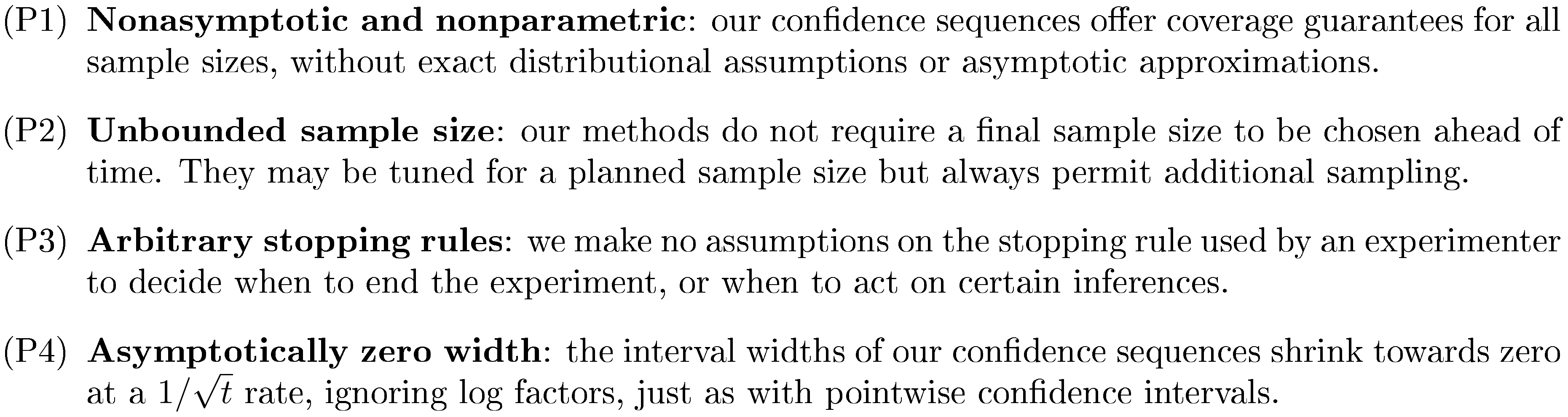
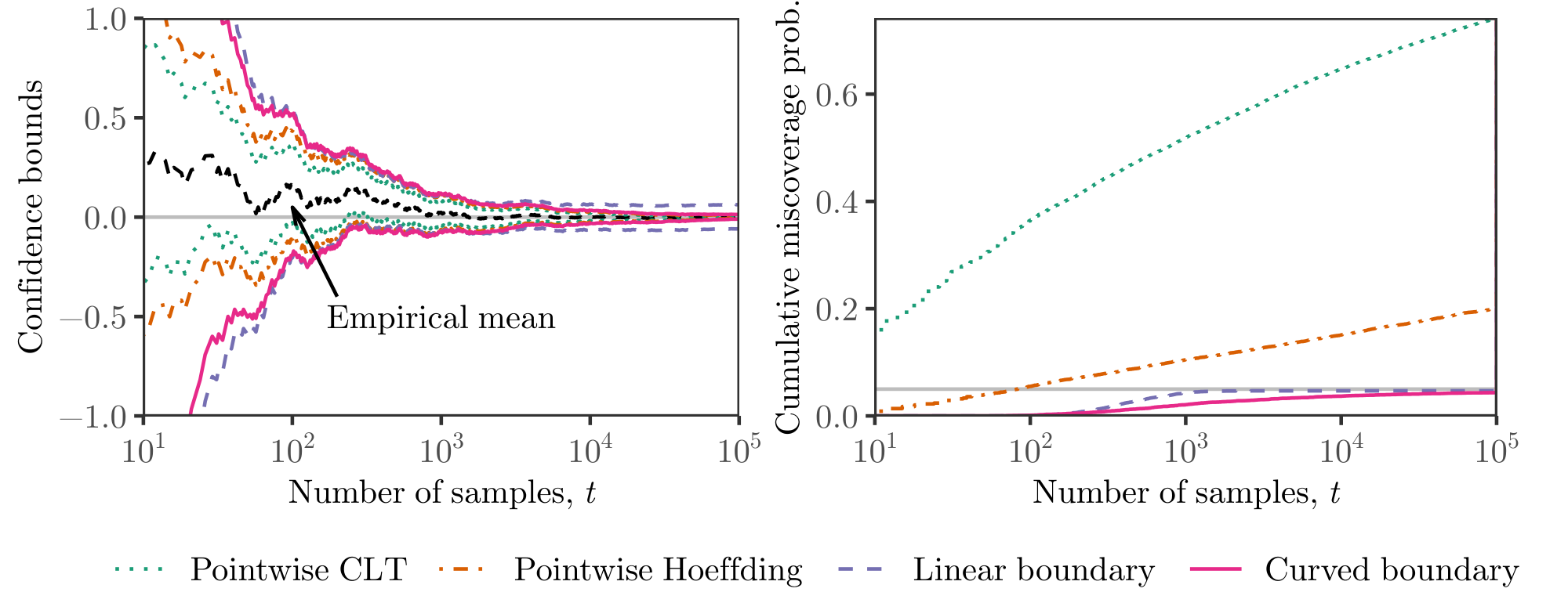
These properties give us strong guarantees and broad applicability. An experimenter may always choose to gather more samples, and may stop at any time according to any rule—the resulting inferential guarantees hold under the stated assumptions without any approximations. Of course, this flexibility comes with a cost: our intervals are wider than those that rely on asymptotics or make stronger assumptions, for example, a known stopping rule. Typical, fixed-sample confidence intervals derived from the central limit theorem do not satisfy any of (P1)-(P3), and accommodating any one property necessitates wider intervals; we illustrate this in Figure 1. It is perhaps surprising that these four properties come at a numerical cost of less than doubling the fixed-sample, asymptotic interval width—the discrete mixture bound illustrated in Figure 9 stays within a factor of two of the fixed-sample CLT bounds over five orders of magnitude in time.

1.1 Related work

The idea of a confidence sequence goes back at least to [3]. They are called repeated confidence intervals by [8, 5] (with a focus on finite time horizons) and always-valid confidence intervals by [9]. They are sometimes labeled anytime confidence intervals in the machine learning literature ([10]).

Prior work on sequential inference is often phrased in terms of a sequential hypothesis test, defined as a stopping rule and an accept/reject decision variable, or in terms of an always-valid $p$-value ([9]). In Section 6 we discuss the duality between confidence sequences, sequential hypothesis tests, and always-valid $p$-values. We show in Lemma 19 that definition Equation 1 is equivalent to requiring $\mathbb{P}(\theta_\tau \in \textup{CI}_\tau) \geq 1 - \alpha$ for all stopping times $\tau$, or even for all random times $\tau$, not necessarily stopping times. Hence the choice of definition Equation 1 over related definitions in the literature is one of convenience.

Recent interest in confidence sequences has come from the literature on best-arm identification with fixed confidence for multi-armed bandit problems. [11], [7], [12], and [13] present methods satisfying properties (P1)-(P4) for independent, sub-Gaussian observations. Our results are sharper and more general, and our Bernstein confidence sequence scales with the true variance in nonparametric settings. Confidence sequences are a key ingredient in best-arm selection algorithms ([14]) and related methods for sequential testing with multiple comparisons ([15, 16, 10]). Our results improve and generalize such methods.

[17] and [18] prove empirical-Bernstein bounds for fixed times or finite time horizons. Our empirical-Bernstein bound holds uniformly over infinite time. [19] takes a different approach to deriving confidence sequences satisfying properties (P1)-(P4) by lower bounding a mixture martingale. This work was extended in [20] to an empirical-Bernstein bound, the only infinite-horizon, empirical-Bernstein confidence sequence we are aware of in prior work. Our result removes a multiplicative pre-factor and yields sharper bounds. We emphasize that our proof technique is quite different from all three of these existing empirical-Bernstein bounds; see Appendix A.8.

The simplest confidence sequence satisfying properties (P1)-(P3) follows by inverting a suitably formulated sequential probability ratio test (SPRT, ([21])), such as in Section 3.6 of [6]. Wald worked in a parametric setting, though it is known that the normal SPRT depends only on sub-Gaussianity (e.g., [22]). The resulting confidence sequence does not shrink towards zero width as $t \to \infty$ (property P4), a problem which stems from the choice of a single point alternative $\lambda$. Numerous extensions have been developed to remedy this defect, and our work is most closely tied to two approaches. First, in the method of mixtures, one replaces the likelihood ratio with a mixture $\int \prod_i [f_\lambda(X_i) / f_0(X_i)] \mathop{}!\mathrm{d} F(\lambda)$, which is still a martingale ([23, 21, 24, 25, 26, 22, 27, 28, 19, 29, 30]). Second, epoch-based analyses choose a sequence of point alternatives $\lambda_1, \lambda_2, \dots$ approaching the null value, with corresponding error probabilities $\alpha_1, \alpha_2, \dots$ approaching zero so that a union bound yields the desired error control ([31, 32, 12]).

The literature on self-normalized bounds makes extensive use of the method of mixtures, sometimes called pseudo-maximization ([33, 28, 34, 35, 11]); these works introduced the idea of using a mixture to bound a quantity with a random intrinsic time $V_t$. These results are mostly given for fixed samples or finite time horizon, though [33], Eq. 4.20 includes an infinite-horizon curve-crossing bound. [27] treats confidence sequences for the parameter of an exponential family using mixture techniques similar to those of Section 3.2. Like most work on the method of mixtures, Lai's work focused on the parametric setting (which we discuss in Section 4.4), while we focus on the application of mixture bounds to nonparametric settings.

[36] adopt the mixture approach for a commercial A/B testing platform, where properties (P2) and (P3) are critical to provide an "off-the-shelf" solution for a variety of clients. Their application relies on asymptotics which lack rigorous justification. In Section 4.2 we give nonasymptotic justification for a similar confidence sequence under a finite-sample randomization inference model, and in Section 5 we demonstrate how our methods control Type I error in situations where asymptotics fail.

1.2 Outline

We organize our results using the sub-Gaussian, sub-gamma, sub-Bernoulli, sub-Poisson and sub-exponential settings defined in Section 2.

1. The stitching method gives new closed-form sub-Gaussian or sub-gamma boundaries (Theorem 5). Our sub-gamma treatment extends prior sub-Gaussian work to cover any martingale whose increments have finite moment-generating function in a neighborhood of zero; see Proposition 3. Our proof is transparent and flexible, accommodating a variety of boundary shapes, including those growing at the rate $\mathcal{O}(\sqrt{t \log \log t})$ with a focus on tight constants, though we do not recommend this bound in practice unless closed-form simplicity is vital.
2. Conjugate mixtures give one- and two-sided boundaries for the sub-Bernoulli, sub-Gaussian, sub-Poisson and sub-exponential cases (Section 3.2) which avoid approximations made for analytical convenience. The sub-Gaussian boundaries are unimprovable without further assumptions (Section 3.6). These boundaries include a common tuning parameter which is critical in practice and we discuss why their $\mathcal{O}(\sqrt{t \log t})$ growth rate may be preferable to the slower $\mathcal{O}(\sqrt{t \log \log t})$ rate (Section 3.5).
3. Discrete mixtures facilitate numerical computation of boundaries with a great deal of flexibility, at the cost of slightly more involved computations (Theorem 9). Like conjugate mixture boundaries, these boundaries avoid unnecessary approximations and are unimprovable in the sub-Gaussian case.
4. Finally, for sub-Gaussian processes, the inverted stitching method (Theorem 10) gives numerical upper bounds on the crossing probability of any increasing, strictly concave boundary over a limited time range. We show that any such boundary yields a uniform upper tail inequality over a finite horizon, and compute its crossing probability.

Building on this foundation, we present a a state-of-the-art empirical-Bernstein bound (Theorem 13) for any sequence of bounded observations using a new self-normalization proof technique. We illustrate our methods with two novel applications: the nonasymptotic, sequential estimation of average treatment effect in the Neyman-Rubin potential outcomes model (Section 4.2), and the derivation of uniform matrix bounds and covariance matrix confidence sequences (Corollary 15 and Section 4.3). We give simulation results in Section 5. Section 6 discusses the relationship of our work to existing concepts of sequential testing. Proofs of main results are in Appendix A, with others deferred to Appendix C.

2. Preliminaries: linear boundaries

Section Summary: This section explains how to estimate the average expected value of a sequence of observations over time using a running sample mean, while accounting for deviations from those expectations through a process called S_t. To create reliable lower bounds for these estimates—known as confidence sequences—it focuses on uniform upper tail probabilities for S_t, scaled by an "intrinsic time" process V_t that tracks squared deviations, without assuming the observations are independent or have the same mean. The approach builds on a mathematical condition called the sub-ψ property, rooted in martingale techniques from probability theory, which ensures the exponential growth of deviations can be controlled like a supermartingale to derive these bounds.

Given a sequence of real-valued observations $(X_t){t=1}^\infty$, suppose we wish to estimate the average conditional expectation $\mu_t \coloneqq t^{-1} \sum{i=1}^t \mathbb{E}{i-1} X_i$ at each time $t$ using the sample mean $\bar{X}t \coloneqq t^{-1} \sum{i=1}^t X_i$; here we assume an underlying filtration $(\mathcal{F}t){t=1}^\infty$ to which $(X_t)$ is adapted, and $\mathbb{E}t$ denotes expectation conditional on $\mathcal{F}t$. Let $S_t \coloneqq \sum{i=1}^t (X_i - \mathbb{E}{i-1} X_i)$, the zero-mean deviation of our sample sum from its estimand at time $t$. Given $\alpha \in (0, 1)$, suppose we can construct a uniform upper tail bound $u\alpha: \mathbb{R}{\geq 0} \to \mathbb{R}{\geq 0}$ satisfying

$ \begin{align} \mathbb{P}\big(\exists t \geq 1 : S_t \geq u_\alpha(V_t)\big) \leq \alpha \end{align}\tag{3} $

for some adapted, real-valued intrinsic time process $(V_t){t=1}^\infty$, an appropriate time scale to measure the (squared) deviations of $(S_t)$. This uniform upper bound on the centered sum $(S_t)$ yields a lower confidence sequence for $(\mu_t)$ with radius $t^{-1} u\alpha(V_t)$: $\mathbb{P}\left(\forall t \geq 1 : \bar{X}t - t^{-1} u\alpha(V_t) \leq \mu_t \right) \geq 1 - \alpha$.

Note that an assumption on the upper tail of $(S_t)$ yields a lower confidence sequence for $(\mu_t)$; a corresponding assumption on the lower tail of $(S_t)$ yields an upper confidence sequence for $(\mu_t)$. In this paper we formally focus on upper tail bounds, from which lower tail bounds can be derived by examining $(-S_t)$ in place of $(S_t)$. In general, the left and right tails of $(S_t)$ may behave differently and require different sets of assumptions, so that our upper and lower confidence sequences may have different forms. Regardless, we can always combine upper and lower confidence sequences using a union bound to obtain a two-sided confidence sequence Equation 1.

When the $(X_t)$ are independent with common mean $\mu$, the resulting confidence sequence estimates $\mu$, but the setup requires neither independence nor a common mean. In general, the estimand $\mu_t$ may be changing at each time $t$; Section 4.2 gives an application to causal inference in which this changing estimand is useful. In principle, $\mu_t$ may also be random, although none of our applications involve random $\mu_t$.

To construct uniform boundaries $u_\alpha$ satisfying inequality Equation 3, we build upon the following general condition ([6], Definition 1):

########## {caption="Definition 1: Sub- $\psi$ condition"}

Let $\smash{(S_t){t = 0}^\infty, (V_t){t = 0}^\infty}$ be real-valued processes adapted to an underlying filtration $(\mathcal{F}t){t = 0}^\infty$ with $\smash{S_0=V_0=0}$ and $\smash{V_t\geq0}$ for all $t$. For a function $\psi: [0, \lambda_{\max}) \to \mathbb{R}$ and a scalar $l_0 \in [1, \infty)$, we say $(S_t)$ is $l_0$-sub- $\psi$ with variance process $(V_t)$ if, for each $\lambda \in [0, \lambda_{\max})$, there exists a supermartingale $(L_t(\lambda))_{t = 0}^\infty$ w.r.t. $(\mathcal{F}_t)$ such that $\mathbb{E} L_0(\lambda) \leq l_0$ and

$ \begin{align} \exp \left\lbrace \lambda S_t - \psi(\lambda) V_t \right\rbrace \leq L_t(\lambda) \text{ a.s.\ for all } t. \end{align} $

For given $\psi$ and $l_0$, let $\mathbb{S}^{l_0}_{\psi}$ be the class of pairs of $l_0$-sub- $\psi$ processes $(S_t, V_t)$:

$ \begin{align} \mathbb{S}^{l_0}_{\psi} \coloneqq \left\lbrace (S_t, V_t): (S_t) \text{ is $l_0$-sub-$\psi$ with variance process } (V_t) \right\rbrace. \end{align} $

When stating that a process is sub- $\psi$, we typically omit $l_0$ from our terminology for simplicity. In scalar cases, we always have $l_0 = 1$, while in matrix cases $l_0 = d$, the dimension of the (square) matrices.

Where does Definition 1 come from? The jumping-off point is the martingale method for concentration inequalities (([37, 38, 39]); ([40], section 2.2)), itself based on the classical Cramér-Chernoff method (([41, 42]); ([43], section 2.2)). The martingale method starts off with an assumption of the form $\mathbb{E}{t-1}e^{\lambda(X_t - \mathbb{E}{t-1} X_t)}\leq e^{\psi(\lambda)\sigma_t^2}$ for all $t \geq 1, \lambda \in \mathbb{R}$. Then, denoting $S_t \coloneqq \sum_{i=1}^t (X_i - \mathbb{E}{i-1} X_i)$ and $V_t \coloneqq \sum{i=1}^t \sigma_i^2$, the process $\exp \left\lbrace \lambda S_t - \psi(\lambda) V_t \right\rbrace$ is a supermartingale for each $\lambda \in \mathbb{R}$. Unlike the martingale method assumption, Definition 1 allows the exponential process to be upper bounded by a supermartingale, and it permits $(V_t)$ to be adapted rather than predictable. We also restrict our attention to $\lambda \geq 0$ to derive one-sided bounds.

Intuitively, the process $\exp \left\lbrace \lambda S_t - \psi(\lambda) V_t \right\rbrace$ measures how quickly $S_t$ has grown relative to intrinsic time $V_t$, and the free parameter $\lambda$ determines the relative emphasis placed on the tails of the distribution of $S_t$, i.e., on the higher moments. Larger values of $\lambda$ exaggerate larger movements in $S_t$, and $\psi$ captures how much we must correspondingly exaggerate $V_t$. $\psi$ is related to the heavy-tailedness of $S_t$ and the reader may think of it as a cumulant-generating function (CGF, the logarithm of the moment-generating function). For example, suppose $(X_t)$ is a sequence of i.i.d., zero-mean random variables with CGF $\psi(\lambda) \coloneqq \log \mathbb{E} e^{\lambda X_1}$ which is finite for all $\lambda \in [0, \lambda_{\max})$. Then, setting $V_t \coloneqq t$, we see that $L_t(\lambda) \coloneqq \exp \left\lbrace \lambda S_t - \psi(\lambda) V_t \right\rbrace$ is itself a martingale, for all $\lambda \in [0, \lambda_{\max})$. Indeed, in all scalar cases we consider, $L_t(\lambda)$ is just equal to $\exp \left\lbrace \lambda S_t - \psi(\lambda) V_t \right\rbrace$. See Appendix Table 3 and Table 4, drawn from [6], for a catalog of sufficient conditions for a process to be sub- $\psi$ using the five $\psi$ functions defined below. We use many of these conditions in what follows.

We organize our uniform boundaries according to the $\psi$ function used in Definition 1. First recall the Cramér-Chernoff bound: if $(X_t)$ are independent zero-mean with bounded CGF $\log \mathbb{E} e^{\lambda X_t} \leq \psi(\lambda)$ for all $t \geq 1$ and $\lambda \in \mathbb{R}$, then writing $S_t = \sum_{i=1}^t X_i$, we have $\mathbb{P}(S_t \geq x) \leq e^{-t \psi^\star(x/t)}$ for any $x > 0$, where $\psi^\star$ denotes the Legendre-Fenchel transform of $\psi$. Equivalently, writing $z_\alpha(t) \coloneqq t {\psi^\star}^{-1}(t^{-1} \log \alpha^{-1})$, we have $\mathbb{P}(S_t \geq z_\alpha(t)) \leq \alpha$ for any fixed $t$ and $\alpha \in (0, 1)$. In other words, the function $z_\alpha$ gives a high-probability upper bound at any fixed time $t$ for any sum of independent random variables with CGF bounded by $\psi$. When we extend this concept to boundaries holding uniformly over time, there is no longer a unique, minimized boundary, and the following definition captures the class of valid boundaries.

########## {caption="Definition 2"}

Given $\smash{\psi: [0, \lambda_{\max}) \to \mathbb{R}}$ and $\smash{l_0\geq 1}$, a function $\smash{u: \mathbb{R}\to \mathbb{R}}$ is called an $l_0$-sub- $\psi$ uniform boundary with crossing probability $\alpha$ if

$ \begin{align} \sup_{(S_t, V_t) \in \mathbb{S}^{l_0}_{\psi}} \mathbb{P}(\exists t \geq 1: S_t \geq u(V_t)) \leq \alpha. \end{align} $

Although $u$ does depend on the constant $l_0$ in Definition 1, for simplicity we typically omit this dependence from our notation, writing simply that $u$ is a sub- $\psi$ uniform boundary.

Five particular $\psi$ functions play important roles in our development; below, we take $1 / 0 = \infty$ in the upper bounds on $\lambda$:

• $\psi_{B, g, h}(\lambda) \coloneqq \frac{1}{gh} \log\left(\frac{ge^{h\lambda} + he^{-g\lambda}}{g+h} \right)$ on $0 \leq \lambda < \infty$, the scaled CGF of a centered random variable (r.v.) supported on two points, $-g$ and $h$, for some $g, h > 0$, for example a centered Bernoulli r.v. when $g + h = 1$.
• $\psi_N(\lambda) \coloneqq \lambda^2/2$ on $0 \leq \lambda < \infty$, the CGF of a standard Gaussian r.v.
• $\psi_{P, c}(\lambda) \coloneqq c^{-2}(e^{c\lambda} - c\lambda - 1)$ on $0 \leq \lambda < \infty$ for some scale parameter $c \in \mathbb{R}$, which is the CGF of a centered unit-rate Poisson r.v. when $c=1$. By taking the limit, we define $\psi_{P, 0} = \psi_N$.
• $\psi_{E, c}(\lambda) \coloneqq c^{-2}(-\log(1-c\lambda) - c\lambda)$ on $0 \leq \lambda < 1 / (c \vee 0)$ for some scale $c \in \mathbb{R}$, which is the CGF of a centered unit-rate exponential r.v. when $c = 1$. By taking the limit, we define $\psi_{E, 0} = \psi_N$.
• $\psi_{G, c}(\lambda) \coloneqq \lambda^2 / (2 (1 - c\lambda))$ on $0 \leq \lambda < 1 / (c \vee 0)$ (taking $1/0 = \infty$) for some scale parameter $c \in \mathbb{R}$, which we refer to as the sub-gamma case following [43]. This is not the CGF of a gamma r.v. but is a convenient upper bound which also includes the sub-Gaussian case at $c = 0$ and permits analytically tractable results below.

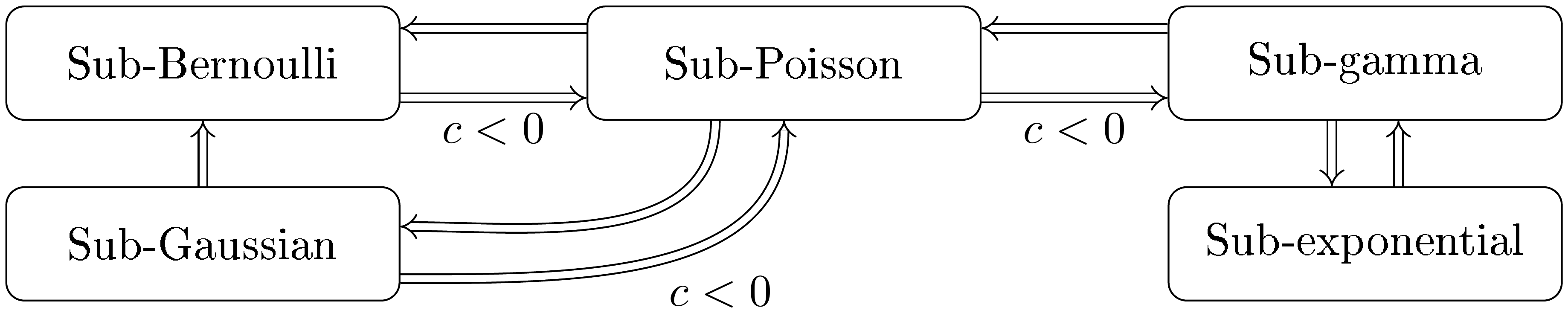
One may freely scale $\psi$ by any positive constant and divide $V_t$ by the same constant so that Definition 1 remains satisfied; by convention, we scale all $\psi$ functions above so that $\psi''(0_+) = 1$. When we speak of a sub-gamma process (or uniform boundary) with scale parameter $c$, we mean a sub- $\psi_{G, c}$ process (or uniform boundary), and likewise for other cases. We often write $\psi_B$, $\psi_P$, etc., dropping the range and scale parameters from our notation. As we summarize in Figure 2 and detail in Proposition 31, certain general implications hold among sub- $\psi$ boundaries. In particular, any sub-Gaussian boundary can also serve as a sub-Bernoulli boundary; any sub-Poisson boundary serves as a sub-Gaussian or sub-Bernoulli boundary; and, importantly, any sub-gamma or sub-exponential boundary can serve as a sub- $\psi$ boundary in any of the other four cases. Indeed, a sub-gamma or sub-exponential boundary applies to many cases of practical interest, as detailed below.

########## {caption="Proposition 3"}

Suppose $\psi$ is twice-differentiable and $\smash{\psi(0) = \psi'(0_+) = 0}$. Suppose, for each $c>0$, $u_c(v)$ is a sub-gamma or sub-exponential uniform boundary with crossing probability $\alpha$ for scale $c$. Then $v \mapsto u_{k_1}(k_2v)$ is a sub- $\psi$ uniform boundary for some constants $k_1, k_2 > 0$ depending only on $\psi$.

Proposition 3 restates [6], Proposition 1, which shows that any process $(S_t)$ which is sub- $\psi$ is also sub-gamma and sub-exponential, if $\psi$ satisfies the conditions of Proposition 3. Note that these conditions are satisfied for any mean-zero random variable if the CGF exists in a neighborhood of zero, so the conditions are quite weak ([44], Theorem 2.3).

########## {#thm:ex_variance caption="Confidence sequence for the variance of a Gaussian distribution

with unknown mean" type="Example"

Suppose $X_1, X_2, \dots$ are i.i.d.\ draws from a $\mathcal{N}(\mu, \sigma^2)$ distribution and we wish to sequentially estimate $\sigma^2$ when $\mu$ is also unknown. Let $S_t \coloneqq \sigma^{-2} \sum_{i=1}^{t+1} (X_i - \bar{X}{t+1})^2 - t$ for $t = 1, 2, \dots$, where $\bar{X}t \coloneqq t^{-1} \sum{i=1}^t X_i$ is the sample mean. This $S_t$ is a centered and scaled sample variance, and as in [3], we use the fact that $S_t$ is a cumulative sum of independent, centered Chi-squared random variables each with one degree of freedom (see Appendix H for details). Such a centered Chi-squared distribution has variance two and CGF equal to $2 \psi{E, 2}$.

Thus $(S_t)$ is 1-sub-exponential with variance process $V_t = 2t$ and scale parameter $c = 2$. We may uniformly bound the upper deviations of $S_t$ using any sub-exponential uniform boundary, for example the gamma-exponential mixture boundary of Proposition 24. Or, we can use Proposition 31 to deduce that $(S_t)$ is sub-gamma with scale $c = 2$ (and the same variance process) and use the closed-form stitched boundary of Theorem 5.

The above constructions yield lower confidence sequences for the variance. To obtain an upper confidence sequence, we use the fact that $(-S_t)$ is 1-sub-exponential with scale parameter $\smash{c = -2}$. Now Proposition 31 implies that $(-S_t)$ is sub-gamma with scale $c = -1$, so the stitched boundary again applies, while Proposition 31 implies that $(-S_t)$ is also sub-Gaussian, so we may alternatively use the normal mixture boundary of Proposition 21. Since $\psi_{G, -1}$ is uniformly smaller than $\psi_N$, the above analysis yields tighter bounds than the sub-Gaussian approach of [3].

The simplest uniform boundaries are linear with positive intercept and slope. This is formalized in [6], partially restated below.

########## {caption="Lemma 4: ([6]), Theorem 1"}

For any $\lambda \in [0, \lambda_{\max})$ and $\alpha \in (0, 1)$,

$ \begin{align} u(v) \coloneqq \frac{\log(l_0 / \alpha)}{\lambda}

• \frac{\psi(\lambda)}{\lambda} \cdot v \end{align} $

is a sub- $\psi$ uniform boundary with crossing probability $\alpha$.

While Lemma 4 provides a versatile building block, the $\mathcal{O}(V_t)$ growth of $u(V_t)$ may be undesirable. Indeed, from a concentration point of view, the typical deviations of $S_t$ tend to be only $\mathcal{O}(\sqrt{V_t})$, so the bound will rapidly become loose for large $t$. From a confidence sequence point of view, recall that the confidence radius for the mean is given by $u(V_t) / t$. Typically, $V_t = \Theta(t)$ a.s. as $t \to \infty$, so the confidence radius will be asymptotically zero width if and only if $u(v) = o(v)$. In other words, we cannot achieve arbitrary estimation precision with arbitrarily large samples unless the uniform boundary is sublinear. We address this problem in Section 3, building upon Lemma 4 to construct curved sub- $\psi$ uniform boundaries.

3. Curved uniform boundaries

Section Summary: This section outlines techniques for computing curved uniform boundaries to control the excursions of random processes, such as sub-Gaussian or sub-gamma ones, which are useful in fields like statistics and machine learning. It focuses on a "stitched" analytical boundary that combines simpler linear bounds across geometrically spaced time periods, requiring user-chosen parameters to set the starting point, growth rate, and overall shape. The method guarantees that the probability of the process crossing this boundary remains below a specified small value, with growth behaving like the square root of time multiplied by the log of log time in key examples, ensuring reliable performance through careful tuning.

We present our four methods for computing curved uniform boundaries in Figure 3, Section 3.2, Figure 8, and Section 3.4. In Section 3.5, we discuss how to tune boundaries, a necessity for good performance in practice, and we describe the unimprovability of sub-Gaussian mixture bounds in Section 3.6.

3.1 Closed-form boundaries via stitching

Our analytical "stitched" bound is useful in the sub-Gaussian case or, more generally, the sub-gamma case with scale $c$. We require three user-chosen parameters:

• a scalar $\eta > 1$ determines the geometric spacing of intrinsic time,
• a scalar $m > 0$ which gives the intrinsic time at which the uniform boundary starts to be nontrivial, and
• an increasing function $h : \mathbb{R}{\geq 0} \to \mathbb{R}{>0}$ such that ${\sum_{k=0}^\infty 1 / h(k) \leq 1}$, which determines the shape of the boundary's growth after time $m$.

Recalling the scale parameter $c$ for the $\psi_G$ function above and the constant $l_0$ in Definition 1, we define the stitching function $\mathcal{S}_\alpha$ as

$ \mathcal{S}_\alpha(v) \coloneqq \sqrt{k_1^2 v \ell(v) + k_2^2 c^2 \ell^2(v)} \

• k_2 c \ell(v), \text{ where } \begin{cases} \ell(v) \coloneqq \log h(\log_{\eta}(\frac{v}{m})) + \log(\frac{l_0}{\alpha}), \ k_1 \coloneqq (\eta^{1/4} + \eta^{-1/4}) / \sqrt{2}, \ k_2 \coloneqq (\sqrt{\eta} + 1) / 2, \end{cases}\tag{4} $

and define the stitched boundary as $u(v) = \mathcal{S}\alpha(v \vee m)$. Note $\mathcal{S}\alpha(v) \leq k_1 \sqrt{v \ell(v)} + 2 c k_2 \ell(v)$ when $c > 0$, while $\mathcal{S}\alpha(v) \leq k_1 \sqrt{v \ell(v)}$ when $c \leq 0$, with equality in the sub-Gaussian case ($c = 0$). These simpler expressions may sometimes be preferable. For notational simplicity we suppress the dependence of $\mathcal{S}\alpha$ on $h$, $\eta$, $l_0$, and $c$; we will discuss specific choices as necessary. In the examples we consider, $\ell(v)$ grows as $\mathcal{O}(\log v)$ or $\mathcal{O}(\log \log v)$ as $v \uparrow \infty$, so the first term, $k_1 \sqrt{V_t \ell(V_t)}$, dominates for sufficiently large $V_t$, specifically when $V_t / \ell(V_t) \gg 2c^2\sqrt{\eta}$.

########## {caption="Theorem 5: Stitched boundary"}

For any $\smash{c \geq 0, \alpha \in (0, 1), \eta > 1, m>0}$, and $\smash{h : \mathbb{R}{\geq 0} \to \mathbb{R}{\geq 0}}$ increasing such that $\smash{\sum_{k=0}^\infty 1 / h(k) \leq 1}$, the function $v \mapsto \mathcal{S}_\alpha(v \vee m)$ is a sub-gamma uniform boundary with crossing probability $\alpha$. Further, for any sub- $\psi_G$ process $(S_t)$ with variance process $(V_t)$ and any $v_0 \geq m$,

$ \begin{align} \mathbb{P}\left(\exists t \geq 1: V_t \geq v_0 \text{ and } S_t \geq \mathcal{S}\alpha(V_t) \right) \leq \sum{k=\lfloor \log_\eta(v_0/m) \rfloor}^\infty \frac{\alpha}{h(k)}. \end{align}\tag{5} $

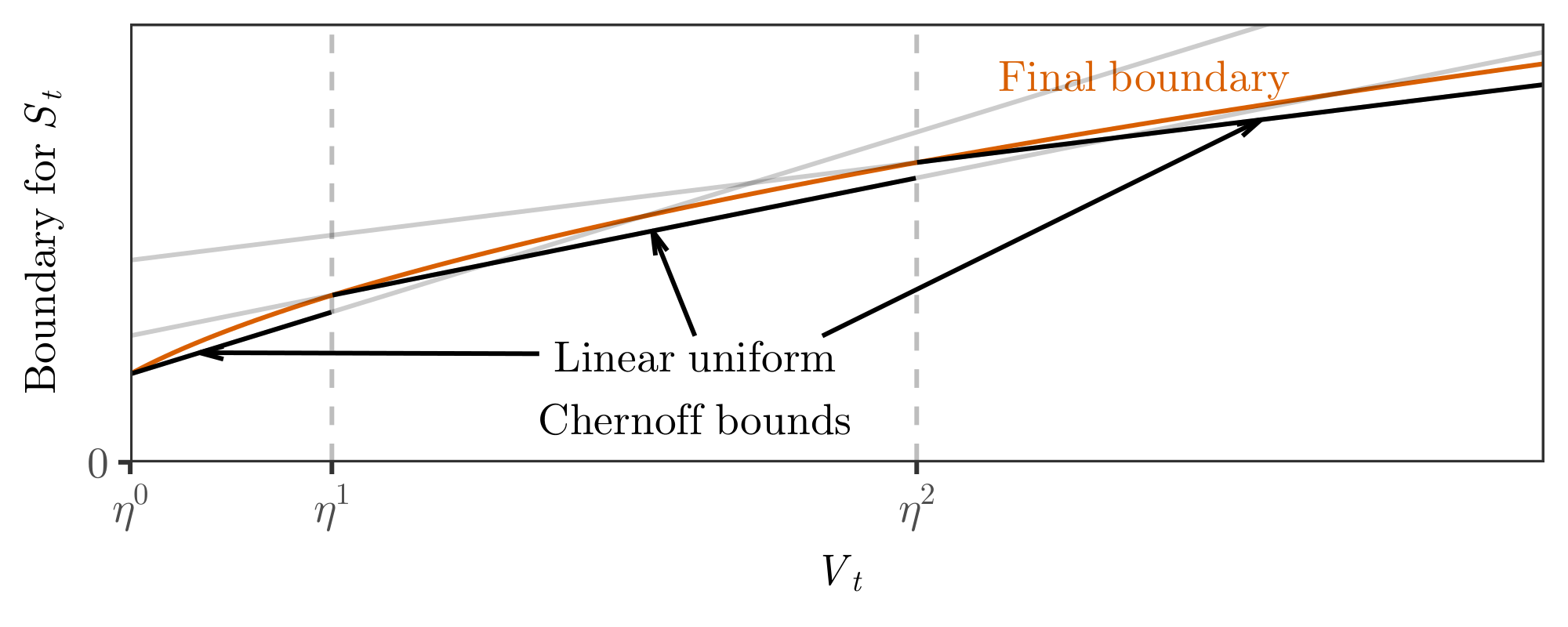
The first sentence above says that the probability of $S_t$ crossing $\mathcal{S}\alpha(V_t \vee m)$ at least once is at most $\alpha$, while the second says that, even if it does happen to cross once or more, the probability of further crossings decays to zero beyond larger and larger intrinsic times $v_0$. Note that Equation 5 implies $\mathbb{P}\left(\sup_t V_t = \infty and S_t \geq \mathcal{S}\alpha(V_t) infinitely often \right) = 0$. The proof of Theorem 5, given with discussion in Appendix A.1, follows by taking a union bound over a carefully chosen family of linear boundaries, one for each of a sequence of geometrically-spaced epochs; see Figure 3. The high-level proof technique is standard, often referred to as "peeling" in the bandit literature, and closely related to chaining elsewhere in probability theory. Our proof generalizes beyond the sub-Gaussian case and involves careful parameter choices in order to achieve tight constants. In brief, within each epoch, there are many possible linear boundaries, and we have found that optimizing the linear boundary for the geometric mean of the epoch endpoints strikes a good balance between tight constants and analytical simplicity in the final boundary. Appendix G gives a detailed comparison of constants arising from our bound with similar bounds from the literature.

The boundary shape is determined by choosing the function $h$ and setting the nominal crossing probability in the $k$ $^{\text{th}}$ epoch to equal $\alpha/h(k)$. Then Theorem 5 gives a curved boundary which grows at a rate $\mathcal{O}\left(\sqrt{V_t \log h(\log_\eta V_t)} \right)$ as $V_t \uparrow \infty$. The more slowly $h(k)$ grows as $k \uparrow \infty$, the more slowly the resulting boundary will grow as $V_t \uparrow \infty$. A simple choice is exponential growth, $h(k) = \eta^{sk} / (1 - \eta^{-s})$ for some $s > 1$, yielding $\mathcal{S}_\alpha(v) = \mathcal{O}(\sqrt{v \log v})$. A more interesting example is $h(k) = (k + 1)^s \zeta(s)$ for some $s > 1$, where $\zeta(s)$ is the Riemann zeta function. Then, when $l_0 = 1$, Theorem 5 yields the polynomial stitched boundary: for $c \geq 0$,

$ \begin{align} \mathcal{S}_\alpha(v) = k_1 \sqrt{ v \left(s \log\log\left(\frac{\eta v}{m} \right)

• \log \frac{\zeta(s)}{\alpha \log^s \eta} \right) }
• c k_2 \left(s \log\log\left(\frac{\eta v}{m} \right)
• \log \frac{\zeta(s)}{\alpha \log^s \eta} \right), \end{align}\tag{6} $

where the second term is neglected in the sub-Gaussian case since $c=0$. This is a "finite LIL bound", so-called because $\mathcal{S}_\alpha(v) \sim \sqrt{s k_1^2 v \log \log v}$, matching the form of the law of the iterated logarithm ([45]). We can bring $s k_1^2$ arbitrarily close to $2$ by choosing $\eta$ and $s$ sufficiently close to one, at the cost of inflating the additive term $\log(\zeta(s) / (\log^s \eta))$. Briefly, increasing $\eta$ increases the size of each epoch in the aforementioned peeling argument, which reduces the looseness of the union bound over epochs. But the larger we make the epochs, the further each linear boundary deviates from the ideal curved shape at the ends of the epochs, which inflates our final boundary. The choice of $s$ involves a similar tradeoff: increasing $s$ causes us to exhaust more of our total error probability budget on earlier epochs, decreasing the constant term (which matters most for early times), at the cost of a union bound over smaller error probabilities in later epochs, which shows up as an increase in the leading constant. We discuss parameter tuning in more practical terms in Section 3.5. For example, take $\smash{\eta = 2, s = 1.4, m = 1}$; if $S_t$ is a sum of independent, zero-mean, 1-sub-Gaussian observations, we obtain

$ \begin{align} \mathbb{P}\left(\exists t \geq 1 : S_t \geq 1.7 \sqrt{t \left(\log \log(2t) + 0.72 \log \left(\frac{5.2}{\alpha} \right) \right)} \right) \leq \alpha. \end{align}\tag{7} $

Figure 9 in Appendix G compares a sub-Gaussian stitched boundary to a numerically-computed discrete mixture bound with a mixture distribution roughly corresponding to $h(k) \propto (k+1)^{1.4}$, as described in Appendix A.6. This discrete mixture boundary acts as a lower bound (see Section 3.6) and shows that not too much is lost by the approximations involved in the stitching construction. Figure 10 compare the same stitched boundary to related bounds from the literature; our bound shows slightly improved constants over the best known bounds.

Although our stitching construction begins with a sub-gamma assumption, it applies to other sub- $\psi$ cases, including sub-Bernoulli, sub-Poisson and sub-exponential cases; see Figure 2 and Proposition 3. Further, our stitched bounds apply equally well in continuous-time settings to Brownian motion, continuous martingales, martingales with bounded jumps, and martingales whose jumps satisfy a Bernstein condition; see Corollary 35.

While our focus is on nonasymptotic results, Theorem 5 makes it easy to obtain the following general upper asymptotic LIL, proved in Appendix A.2:

########## {caption="Corollary 6"}

Suppose $(S_t)$ is sub- $\psi$ with variance process $(V_t)$ and $\psi(\lambda) \sim \lambda^2 / 2$ as $\lambda \downarrow 0$. Then

$ \begin{align} \limsup_{t \to \infty} \frac{S_t}{\sqrt{2 V_t \log \log V_t}} \leq 1 \quad \text{on } \left\lbrace \sup_t V_t = \infty \right\rbrace. \end{align} $

3.2 Conjugate mixture boundaries

For appropriate choice of mixing distribution $F$, the integral $\int \exp \left\lbrace \lambda S_t - \psi(\lambda) V_t \right\rbrace \mathop{}!\mathrm{d} F(\lambda)$ will be analytically tractable. Since, under Definition 1, this mixture process is upper bounded by a mixture supermartingale $\int L_t(\lambda) \mathop{}!\mathrm{d} F(\lambda)$, such mixtures yield closed-form or efficiently computable curved boundaries, which we call conjugate mixture boundaries. This approach is known as the method of mixtures, one of the most widely-studied techniques for constructing uniform bounds ([23, 21, 24, 22, 25, 26, 27, 30]). Unlike the stitched bound of Theorem 5, which involves a small amount of looseness in the analytical approximations, mixture boundaries involve no such approximations and, in the sub-Gaussian case, are unimprovable in the sense described in Section 3.6. We restate the following standard idea behind the method of mixtures using our definitions, with a proof in Appendix A.3. The proof details a technical condition on product measurability which we require of $L_t$.

########## {caption="Lemma 7"}

For any probability distribution $F$ on $[0, \lambda_{\max})$ and $\alpha \in (0, 1)$,

$ \begin{align} \mathcal{M}\alpha(v) := \sup\Bigg\lbrace s \in \mathbb{R}: \underbrace{\int \exp \left\lbrace \lambda s - \psi(\lambda) v \right\rbrace \mathop{}!\mathrm{d} F(\lambda)}{\eqqcolon m(s, v)} < \frac{l_0}{\alpha} \Bigg\rbrace \end{align}\tag{8} $

is a sub- $\psi$ uniform boundary with crossing probability $\alpha$, so long as the supermartingale $(L_t)$ of Definition 1 is product measurable when the underlying probability space is augmented with the independent random variable $\lambda$.

For each of our conjugate mixture bounds, we compute $m(s, v)$ in closed-form. The boundary $u(v)$ can then be computed by numerically solving the equation $m(s, v) = l_0 / \alpha$ in $s$, as we show in Appendix D. When an identical sub- $\psi$ condition applies to $(-S_t)$ as well as $(S_t)$, we may apply a uniform boundary to both tails and take a union bound, obtaining a two-sided confidence sequence. However, mixing over $\lambda \in \mathbb{R}$ rather than $\lambda \in \mathbb{R}_{\geq 0}$ yields a two-sided bound directly, so in some cases we present two-sided variants along with their one-sided counterparts. We give details for the following conjugate mixture boundaries in Appendix A.3:

• one-, two-sided normal mixture boundaries (sub-Gaussian case);
• one-, two-sided beta-binomial mixture boundaries (sub-Bernoulli case);
• one-sided gamma-Poisson mixture boundary (sub-Poisson case); and
• one-sided gamma-exponential mixture boundary (sub-exponential case).

The two-sided normal mixture boundary has a closed form expression:

$ \begin{align} u(v) \coloneqq \sqrt{ (v + \rho) \log\left(\frac{l_0^2 (v + \rho)}{\alpha^2 \rho} \right) }. \end{align}\tag{9} $

The one-sided normal mixture boundary has a similar, closed-form upper bound, making these especially convenient. It is clear from Equation 9 that the normal mixture boundary grows as $\mathcal{O}(\sqrt{v \log v})$ asymptotically, and this rate is shared by all of our conjugate mixture boundaries. Indeed, Proposition 8 below, proved in Appendix A.4, shows that such a rate holds for any mixture boundary as given by Equation 8 whenever the mixing distribution is continuous with positive density at and around the origin, a property which holds for all mixture distributions used in our conjugate mixture boundaries, subject to regularity conditions on $\psi$ which hold for the CGF of any nontrivial, mean-zero r.v. and specifically for the five $\psi$ functions in Section 2.

########## {caption="Proposition 8"}

Assume $(i)$ $\psi$ is nondecreasing, $\psi(0) = \psi'(0_+) = 0$, $\psi''(0_+) = c > 0$, and $\psi$ has three continuous derivatives on a neighborhood including the origin; and $(ii)$ $F$ has density $f$ (w.r.t. Lebesgue) which is continuous and positive on a neighborhood including the origin. Then

$ \begin{align} \mathcal{M}_\alpha(v) = \sqrt{ v \left[c\log\left(\frac{c l_0^2 v}{2\pi \alpha^2 f^2(0)} \right) + o(1) \right]} \quad \text{as } v \to \infty. \end{align}\tag{10} $

Note that $f$ need not place mass on all of $[0, \lambda_{\max})$, only near the origin, for the asymptotic rate to hold. Proposition 8 shows how the asymptotic behavior of any such mixture bound depends only on the behavior of $\psi$ and $f$ near the origin, a result reminiscent of the central limit theorem. Analogous, related results for the sub-Gaussian special case using $\psi(\lambda) = \lambda^2 / 2$ can be found in [26], Section 4 and [46], Theorem 2, in some cases under weaker assumptions on $F$.

In contrast to previous derivations of conjugate mixture boundaries in the literature, all of our conjugate mixture boundaries include a common tuning parameter $\rho > 0$ which controls the sample size for which the boundary is optimized. Such tuning is critical in practice, as we explain in Section 3.5, but has been ignored in much prior work. Additionally, with the exception of the sub-Gaussian case, most prior work on the method of mixtures has focused on parametric settings. We instead emphasize the applicability of these bounds to nonparametric settings. For example, when the observations are bounded, one may construct a confidence sequence making use of empirical-Bernstein estimates (Theorem 13) based on our gamma-exponential mixture (Proposition 24). See Appendix J for other conditions in which mixture bounds yield nonparametric uniform boundaries.

3.3 Numerical bounds using discrete mixtures

In applications, one may not need an explicit closed-form expression so long as the bound can be easily computed numerically. Our discrete mixture method is an efficient technique for numerical computation of curved boundaries for processes satisfying Definition 1. It permits arbitrary mixture densities, thus producing boundaries growing at the rate $\mathcal{O}(\sqrt{v \log \log v})$. Recall that the shape of the stitched bound was determined by the user-specified function $h$. For the discrete mixture bound, one instead specifies a probability density $f$ over finite support $(0, \overline{\lambda}]$ for some $\overline{\lambda} \in (0, \lambda_{\max})$. We first discretize $f$ using a series of support points $\lambda_k$, geometrically spaced according to successive powers of some $\eta > 1$, and an associated set of weights $w_k$:

$ \begin{align} \lambda_k \coloneqq \frac{\overline{\lambda}}{\eta^{k+1/2}} \quad \text{and} \quad w_k \coloneqq \frac{\overline{\lambda} (\eta - 1) f(\lambda_k\sqrt{\eta})}{\eta^{k+1}} \quad \text{for} \quad k = 0, 1, 2, \dots. \end{align}\tag{11} $

########## {caption="Theorem 9: Discrete mixture bound"}

Fix $\psi: [0, \lambda_{\max}) \to \mathbb{R}$, $\alpha\in(0, 1)$, $\overline{\lambda} \in (0, \lambda_{\max})$, and a probability density $f$ on $(0, \overline{\lambda}]$ that is nonincreasing and positive. For supports $\lambda_k$ and weights $w_k$ defined in Equation 11,

$ \textup{DM}\alpha(v) \coloneqq \sup\left\lbrace s \in \mathbb{R} : \sum{k=0}^\infty w_k \exp \left\lbrace \lambda_k s - \psi(\lambda_k) v \right\rbrace < \frac{l_0}{\alpha} \right\rbrace,\tag{12} $

is a sub- $\psi$ uniform boundary with crossing probability $\alpha$.

We suppress the dependence of $\textup{DM}_\alpha$ on $f$, $l_0$, $\overline{\lambda}$ and $\eta$ for notational simplicity. Though Theorem 9 is a straightforward consequence of the method of mixtures, our choice of discretization Equation 11 makes it effective, broadly applicable, and easy to implement. See Appendix A.5 for the proof of this result. Figure 9 includes an example bound, demonstrating a slight advantage over stitching. Appendix A.6 describes a connection between the stitching and discrete mixture methods, including a correspondence between the alpha-spending function $h$ and the mixture density $f$. Finally, we note that the method can be applied even when $f$ is not monotone; one must simply choose the discretization Equation 11 more carefully, using known properties of $f$.

3.4 Inverted stitching for arbitrary boundaries

In the method of mixtures, we choose a mixing distribution $F$ and the machinery yields a boundary $\mathcal{M}\alpha$. Likewise, in the stitching construction of Theorem 5, we choose an error decay function $h$ and obtain a boundary $\mathcal{S}\alpha$. Here, we invert the procedure: we choose a boundary function $g(v)$ and numerically compute an upper bound on its $S_t$-upcrossing probability using a stitching-like construction.

########## {caption="Theorem 10"}

For any nonnegative, strictly concave function $g:~ \mathbb{R} \to \mathbb{R}$ and $v_{\max} > 1$, the function

$ \begin{align} u(v) \coloneqq \begin{cases} g(1 \vee v), & v \leq v_{\max}, \ \infty, & \text{otherwise} \end{cases} \end{align}\tag{13} $

is a sub-Gaussian uniform boundary with crossing probability at most

$ \begin{align} l_0 \inf_{\eta > 1} \sum_{k=0}^{\lceil \log_\eta v_{\max} \rceil} \exp \left\lbrace -\frac{2(g(\eta^{k+1}) - g(\eta^k))(\eta g(\eta^k) - g(\eta^{k+1}))} {\eta^k(\eta - 1)^2} \right\rbrace. \end{align}\tag{14} $

The proof is in Appendix A.7. For simplicity we restrict to the sub-Gaussian case; examination of the proof will show that the method applies in other sub- $\psi$ cases as well, since we simply apply Lemma 4 to appropriately chosen lines, but more involved numerical calculations will be necessary, as the closed-form Equation 14 no longer applies. A similar idea was considered by [24], using a mixture integral approximation instead of an epoch-based construction to derive closed-form bounds. Theorem 10 requires numerical summation but yields tighter bounds with fewer assumptions. As an example, Theorem 10 with $\eta = 2.99$ shows that

$ \begin{align} \mathbb{P}\left(\exists t : 1 \leq V_t \leq 10^{20} \text{ and } S_t \geq 1.7 \sqrt{V_t (\log\log(e V_t) + 3.46)} \right) \leq 0.025. \end{align}\tag{15} $

This boundary is illustrated in Figure 9.

3.5 Tuning boundaries in practice

All uniform boundaries involve a tradeoff of tightness at different intrinsic times: making a bound tighter for some range of times requires making it looser at other times. Roughly speaking, the choice of a uniform boundary involves choosing both what time the bound should be optimized for (e.g., should the bound be tightest around 100 observations or around 100, 000 observations?) as well as how quickly the bound degrades as we move away from the optimized-for time (e.g., if we optimize for 100 samples, will the bound be twice as wide when we reach 1, 000 samples, or will it stay within a factor of two until we reach 1, 000, 000 samples?). A boundary which decays more slowly will necessarily not be as tight around the optimized-for time. In brief, linear boundaries decay the most quickly, conjugate mixture boundaries decay substantially more slowly, and polynomial stitched boundaries decay even more slowly; we feel that mixture boundaries strike a good balance in practice.

Here, we explain how to optimize uniform boundaries for a particular time and discuss the above tradeoff in more detail. Let $W_{-1}(x)$ be the lower branch of the Lambert $W$ function, the most negative real-valued solution in $z$ to $z e^z = x$. Consider the unitless process $S_t / \sqrt{V_t}$, and the corresponding uniform boundary $v \mapsto u(v) / \sqrt{v}$. Since all of our uniform boundaries $u(v)$ have positive intercept at $v = 0$, and all grow at least at the rate $\sqrt{v \log \log v}$ as $v \to \infty$, the normalized boundary $u(v) / \sqrt{v}$ diverges as $v \to 0$ and $v \to \infty$. For the two-sided normal mixture Equation 9, there is a unique time $m$ at which $u(v) / \sqrt{v}$ is minimized; $m$ is proportional to tuning parameter $\rho$ as follows:

########## {caption="Proposition 11"}

Let $u(v)$ be the two-sided normal mixture boundary Equation 9 with parameter $\rho > 0$.

• (a) For fixed $\rho > 0$, the function $v \mapsto u(v) / \sqrt{v}$ is uniquely minimized at $v = m$ with $m$ given by

$ \begin{align} \frac{m}{\rho} = -W_{-1}\left(-\frac{\alpha^2}{e l_0^2} \right) - 1. \end{align}\tag{16} $

• (b) For fixed $m > 0$, the choice of $\rho$ which minimizes the boundary value $u(m)$ is also determined by Equation 16.

The above result is proved in Appendix C.1; it is a matter of elementary calculus, but addresses a question that has received little attention in the literature. Figure 4 includes the normalized versions of two normal mixture boundaries optimized for different times, $m = 300$ and $m = $ 5, 000. Optimizing for the range of values of $V_t$ most relevant in a particular application will yield the tightest confidence sequences. However, as the figure shows, one need not have a very precise range of times, so long as one uses a conservatively low value for $m$, because $u(v) / \sqrt{v}$ grows slowly after time $m$. Indeed, for the normal mixture boundary with $\alpha = 0.05$ and $l_0 = 1$, we have $u(m) / \sqrt{m} \approx 3.0$ and $u(100m) / \sqrt{100m} \approx 3.6$, so that the penalty for being off by two orders of magnitude is modest.

The one-sided normal mixture boundary of Appendix Proposition 21 with crossing probability $\alpha$ is nearly identical to the two-sided normal mixture boundary with crossing probability $2\alpha$, so one may choose $\rho$ as in Proposition 11 with $\alpha$ doubled. For the gamma-exponential mixture and other non-sub-Gaussian uniform boundaries, Proposition 11 provides a good approximation in practice. Figure 4 includes gamma-exponential mixture boundaries with the same $\rho$ values as each corresponding normal mixture boundary. Though the normalized gamma-exponential mixture boundary with $m = 300$ clearly reaches its minimum at $v > m$, this choice of $\rho$ seems reasonable. Discrete mixtures can be similarly tuned by adjusting the precision of the mixing distribution, but require additional considerations (Appendix E).

Comparing the sub-Gaussian stitched boundary, discrete mixture boundary, and normal mixture boundary optimized for $m = 300$ in Figure 4 illustrates another important point for practice: although the normal mixture bound grows more quickly than the others as $v \to \infty$, it remains smaller over about three orders of magnitude. This makes it preferable for many real-world applications, as the longest feasible duration of an experiment is rarely more than two orders of magnitude larger than the earliest possible stopping time. For example, many online experiments run for at least one week to account for weekly seasonality effects, and very few such experiments last longer than 100 weeks. As both the normal mixture and the discrete mixture are unimprovable in general (Section 3.6), the difference is attributable to the choice of mixture, or alternatively, to the fact that the normal mixture trades tightness around the optimized-for time in exchange for looseness at much later times. The lesson is that the $\mathcal{O}(v \log \log v)$ rate, while asymptotically optimal in certain settings and useful for theory and some applications, may not be preferable in all real-world scenarios.

3.6 Unimprovability of uniform boundaries

Definition 2 of a sub- $\psi$ boundary $u$ involves only an upper bound on the $u$-crossing probability of any sub- $\psi$ process $(S_t)$. One may reasonably ask for corresponding lower bounds on the $u$-crossing probability to quantify how tight this boundary is. In the ideal case, we might desire a boundary $u$ such that the true $u$-crossing probability of some process $(S_t)$ is equal to the upper bound. In nonparametric settings, we cannot achieve this goal for every sub- $\psi$ process. However, we might still ask that there exists some sub- $\psi$ process for which the true $u$-crossing probability is arbitrarily close to the upper bound, so that the upper bound on crossing probability is unimprovable in general. That is, we might ask that the inequality on the supremum in Definition 2 holds with equality.

The fact we wish to point out, known in various forms, is that in the scalar, sub-Gaussian case, exact mixture bounds are unimprovable in the above sense. It is in this sense that the discrete mixture bound in Figure 9 provides a lower bound, showing that the sub-Gaussian polynomial stitched bound cannot be improved by much. The following result shows that, for any exact, sub-Gaussian mixture boundary $\mathcal{M}\alpha$, as defined in Lemma 7 for $\psi = \psi_N$, there exists a sub-Gaussian process whose true $\mathcal{M}\alpha$-crossing probability is arbitrarily close to $\alpha$. The result is similar to Theorem 2 of [26], which gives a more general invariance principle, but requires conditions on the boundary that appear difficult to verify for arbitrary mixture boundaries $\mathcal{M}\alpha$. Recall that $\mathbb{S}{\psi_N}^1$ is the class of pairs of processes $(S_t, V_t)$ such that $(S_t)$ is 1-sub-Gaussian with variance process $(V_t)$.

########## {caption="Proposition 12"}

For any exact, 1-sub-Gaussian mixture boundary $\mathcal{M}_\alpha$,

$ \begin{align} \sup_{(S_t, V_t) \in \mathbb{S}{\psi_N}^1} \mathbb{P}(\exists t \geq 1: S_t \geq \mathcal{M}\alpha(V_t)) = \alpha. \end{align} $

We prove Proposition 12 in Appendix C.2. In general, for each $\alpha$ there is an infinite variety of boundaries that are unimprovable in the above sense, differing in when they are loose and tight. These different boundaries will yield confidence sequences which are loose or tight at different sample sizes, or, equivalently, are efficient for detecting different effect sizes. Such a boundary cannot be tightened everywhere without increasing the crossing probability.

4. Applications

Section Summary: This section explores practical uses of a new statistical tool called an empirical-Bernstein confidence sequence, which helps estimate averages from bounded data by adapting to the observed variability rather than relying on worst-case assumptions. It begins by detailing the method's core theorem, which provides anytime-valid confidence intervals around the true average expectation, using predictions like past averages or more sophisticated forecasts to tighten the bounds without needing identical distributions. As an example, the approach is applied to measure average treatment effects in randomized experiments, employing an inverse probability weighting estimator to track causal impacts over time with guaranteed coverage.

After presenting an empirical-Bernstein confidence sequence for bounded observations, we apply our uniform boundaries to causal effect estimation and matrix martingales. We also consider estimation for a general, one-parameter exponential family.

4.1 An empirical-Bernstein confidence sequence

The following novel result is proved in Appendix A.8 using a self-normalization argument, which leads to its attractive simplicity. Recall the estimand $\mu_t \coloneqq t^{-1} \sum_{i=1}^t \mathbb{E}_{i-1} X_i$, the average conditional expectation.

########## {caption="Theorem 13"}

Suppose $X_t \in [a, b]$ a.s. for all $t$. Let $(\widehat{X}_t)$ be any $[a, b]$-valued predictable sequence, and let $u$ be any sub-exponential uniform boundary with crossing probability $\alpha$ for scale $c = b - a$. Then

$ \begin{align} \mathbb{P}\left(\forall t \geq 1: \left\lvert\bar{X}t - \mu_t\right\rvert < \frac{u\left(\sum{i=1}^t (X_i - \widehat{X}_i)^2 \right)}{t} \right) \geq 1 - 2\alpha. \end{align}\tag{17} $

This is an empirical-Bernstein bound because it uses the sum of observed squared deviations to estimate the true variance, much like a classical $t$-test. Hence the confidence radius scales with the true standard deviation for sufficiently large samples, regardless of the support diameter $b - a$, and with no prior knowledge of the true variance. Note also that this bound does not require that observations share a common mean.

The confidence statement Equation 17 holds for any sequence of predictions $(\widehat{X}_i)$, but predictions closer to the conditional expectations, $\widehat{X}i \approx \mathbb{E}{i-1} X_i$, will yield smaller confidence intervals on average. A simple choice is the mean, $\widehat{X}t = (t-1)^{-1} \sum{i=1}^{t-1} X_i$, which will be effective when the samples are i.i.d., for example. But the predictions $(\widehat{X}_i)$ can also make use of trends, seasonality, stratification or regression (in the presence of covariates), machine learning algorithms, or any other information that may aid with prediction.

For an explicit example, assume $X_i \in [0, 1]$ and define the empirical variance as $\widehat{V}t \coloneqq \sum{i=1}^t (X_i - \bar{X}_{i-1})^2$. Invoking Theorem 13 with the polynomial stitched bound Equation 6 using $c=1$, $\eta=2$, $m=1$, and $h(k) \propto k^{1.4}$, we have the following 95%-confidence sequence for $\mu_t$:

$ \begin{align} \smash{ \bar{X}_t \pm \frac{ 1.7 \sqrt{(\widehat{V}_t \vee 1) (\log \log(2(\widehat{V}_t \vee 1)) + 3.8)}

• 3.4 \log \log(2(\widehat{V}_t \vee 1)) + 13 }{t}.} \end{align}\tag{18} $

When a closed form is not required, the gamma-exponential mixture (Proposition 24) may yield tighter bounds than stitching; simulations in Section 5 demonstrate the use of Theorem 13 with this mixture.

4.2 Estimating ATE in the Neyman-Rubin model

As one illustration of Theorem 13, we consider the sequential estimation of average treatment effect under the Neyman-Rubin potential outcomes model ([47, 48, 49]). We imagine a sequence of experimental units, each with real-valued potential outcomes under control and treatment denoted by ${Y_t(0), Y_t(1)}_{t \in \mathbb{N}}$, respectively. These potential outcomes are fixed, but we observe only one outcome for each unit in the experiment. We assign a randomized treatment to each unit, denoted by the $\lbrace 0, 1 \rbrace$-valued random variable $Z_t \in \mathcal{F}t$, observing $Y_t^\textup{obs} \coloneqq Y_t(Z_t)$. Here treatment is assigned by flipping a coin for each subject, with a bias possibly depending on previous observations. This treatment assignment is the only source of randomness. Specifically, let $P_t \coloneqq E{t-1} Z_t$ and suppose $0 < P_t < 1$ a.s. for all $t$; then we permit $P_t$ to vary between individuals and to depend on past outcomes. This accommodates Efron's biased coin design [50] and related covariate balancing methods.

At each step $t$, having treated and observed units $1, \dots, t$, we wish to draw inference about the estimand $\textup{ATE}t \coloneqq t^{-1} \sum{i=1}^t [Y_i(1) - Y_i(0)]$. In particular, we seek a confidence sequence for $(\textup{ATE}t){t=1}^\infty$. To construct our estimator, we may utilize any predictions $\widehat{Y}_t(0)$ and $\widehat{Y}t(1)$ for each unit's potential outcomes; these random variables must be $\mathcal{F}{t-1}$-measurable, for each $t$. We then employ the inverse probability weighting estimator

$ \begin{align} X_t & \coloneqq \widehat{Y}_t(1) - \widehat{Y}_t(0)

• \left(\frac{Z_t - P_t}{P_t(1 - P_t)} \right) (Y_t^\textup{obs} - \widehat{Y}_t(Z_t)), \end{align}\tag{19} $

which is (conditionally) unbiased for the individual treatment effect $Y_t(1) - Y_t(0)$. As with Theorem 13, better predictions will lead to shorter confidence intervals, but the coverage guarantee holds for any choice of predictions, and a reasonable choice would be the average of past observed outcomes. See [51] for a similar strategy for fixed-sample estimation.

We assume bounded potential outcomes; for simplicity we assume $Y_t(k) \in [0, 1]$ for all $t \geq 1, k = 0, 1$, and we assume predictions are likewise bounded. We further assume that treatment probabilities are uniformly bounded away from zero and one. Then, an empirical-Bernstein confidence sequence for $\textup{ATE}_t$ follows from Theorem 13, where we use $\widehat{X}_t = \widehat{Y}_t(1) - \widehat{Y}_t(0)$ so that

$ \begin{align} V_t ~ \coloneqq~ \sum_{i=1}^t (X_i - \widehat{X}i)^2 = \sum{i=1}^t \left(\frac{Z_i - P_i}{P_i(1 - P_i)} \right)^2 (Y_i^\textup{obs} - \widehat{Y}_i(Z_i))^2. \end{align} $

########## {caption="Corollary 14"}

Suppose $P_t \in [p_{\min}, 1 - p_{\min}]$ a.s., $Y_t(k) \in [0, 1]$ and $\widehat{Y}t(k) \in [0, 1]$ for all $t \geq 1, k = 0, 1$. Let $u$ be any sub-exponential uniform boundary with scale $2 / p{\min}$ and crossing probability $\alpha$. Then

$ \begin{align} \mathbb{P}\left(\forall t \geq 1: \left\lvert\bar{X}_t - \textup{ATE}_t\right\rvert < \frac{u(V_t)}{t} \right) \geq 1 - 2\alpha. \end{align} $

For $u$, one may choose the gamma-exponential mixture boundary (Proposition 24) or the stitched boundary Equation 6 with $c=\frac{2}{p_{\min}}$. Figure 5 illustrates our strategy on simulated data. Over the range $t = 100$ to $t = $ 100, 000 displayed, our bound is about twice as wide as the fixed-sample CLT bound, with the ratio growing at a slow $ \mathcal{O}(\sqrt{\log t})$ rate thereafter. Of course the fixed-sample CLT bound provides no uniform coverage guarantee.

4.3 Matrix iterated logarithm bounds

Our second application is the construction of iterated logarithm bounds for random matrix sums and their use in sequential covariance matrix estimation. The curved uniform bounds given in Section 3 may be applied to matrix martingales by taking $(S_t)$ to be the maximum eigenvalue process of the martingale and $(V_t)$ the maximum eigenvalue of the corresponding matrix variance process. [6], Section 2 give sufficient conditions for Definition 1 to hold in this matrix case. Then Theorem 5 yields a novel matrix finite LIL; here we give an example for bounded increments. We denote the space of symmetric, real-valued, $d \times d$ matrices by $\mathbb{S}^d$; $\gamma_{\max}(\cdot)$ denotes the maximum eigenvalue; $\ell_{\eta, s}(v) = s \log\log(\eta v / m) + \log \frac{d, \zeta(s)}{\alpha \log^s \eta}$; and $k_1(\eta), k_2(\eta)$ are defined in Equation 4.

########## {caption="Corollary 15"}

Suppose $(Y_t){t=1}^\infty$ is a $\mathbb{S}^d$-valued matrix martingale such that $\smash{\gamma{\max}(Y_t - Y_{t-1}) \leq b}$ a.s. for all $t$. Let $V_t \coloneqq \gamma_{\max}(\sum_{i=1}^t \mathbb{E}{t-1} (Y_t - Y{t-1})^2)$ and $S_t \coloneqq \gamma_{\max}(Y_t)$. Then for any $\smash{\eta >1, s>1, m>0, \alpha\in(0, 1)}$, we have

$ \mathbb{P}\left(\exists t \geq 1 : S_t \geq k_1(\eta) \sqrt{(V_t \vee m) \ell_{\eta, s}(V_t \vee m)}

• \frac{b k_2(\eta)}{3} \ell_{\eta, s}(V_t \vee m) \right) \leq \alpha.\tag{20} $

The result follows using the polynomial stitched boundary after invoking Fact 1(c) and Lemma 2 of [6] (cf. ([52])), which show that $(S_t)$ is sub-gamma with variance process $(V_t)$, scale $c = b/3$, and $l_0 = d$. Beyond bounded increments, the same bound holds for any sub-gamma process. As evidenced by Proposition 3, this is a very general condition.

Taking $\eta$ and $s$ arbitrarily close to one and using the final result of Theorem 5, we obtain the following asymptotic matrix upper LIL, proved in Appendix A.9. Here we denote the martingale increments by $\Delta Y_t \coloneqq Y_t - Y_{t-1}$.

########## {caption="Corollary 16"}

Let $(Y_t){t=1}^\infty$ be a $\mathbb{S}^d$-valued, square-integrable martingale, and define $V_t = \gamma{\max}\left(\sum_{i=1}^t \mathbb{E}_{i-1} \Delta Y_t^2 \right)$. Then

$ \begin{align} \limsup_{t \to \infty} \frac{\gamma_{\max}\left(Y_t \right)} {\sqrt{2 V_t \log \log V_t}} \leq 1 \quad \text{a.s. on } \left\lbrace \sup_t V_t = \infty \right\rbrace \end{align}\tag{21} $

whenever either (1) the increments $(\Delta Y_t)$ are i.i.d., or (2) the increments $(\Delta Y_t)$ satisfy a Bernstein condition on higher moments: for some $c > 0$, for all $t$ and all $k > 2$, $\mathbb{E}{t-1} (\Delta Y_t)^k \preceq (k!/2) c^{k-2} \mathbb{E}{t-1} \Delta Y_t^2$.

The Bernstein condition holds if the increments are uniformly bounded, $\gamma_{\max}(\Delta Y_t) \leq c$ for some $c > 0$. Also, in the i.i.d. case, $\mathbb{P}(V_t \to \infty) = 1$ and then Equation 21 states that $\smash{\limsup_{t \to \infty} \gamma_{\max}\left(Y_t \right) / \sqrt{2 \gamma_{\max}(\mathbb{E} \Delta Y_1^2) t \log \log t} \leq 1}$, a.s. on $\lbrace \sup_t V_t = \infty \rbrace$. When $d = 1$, this recovers the classical upper LIL, showing that Corollary 16 cannot be improved uniformly, but we are not aware of an appropriate lower bound for the general matrix case.

We now consider the nonasymptotic sequential estimation of a covariance matrix based on bounded vector observations ([53, 54, 55, 56, 57]). In particular, we observe a sequence of independent, mean zero, $\mathbb{R}^d$-valued random vectors $x_t$ with common covariance matrix $\Sigma = \mathbb{E} x_t x_t^T$. We wish to estimate $\Sigma$ using an operator-norm confidence ball centered at the empirical covariance matrix $\widehat{\Sigma}t \coloneqq t^{-1} \sum{i=1}^t x_i x_i^T$. For fixed-sample estimation, when $\lVert x_i\rVert_2 \leq \sqrt{b}$ a.s. for all $i \in [t]$, the analysis of [56], section 1.6.3 implies

$ \begin{align} {\mathbb{P}\left(\lVert\widehat{\Sigma}t - \Sigma\rVert{\text{op}} \geq \sqrt{\frac{2 b \lVert\Sigma\rVert_{\text{op}} \log(2d/\alpha)}{t}}

• \frac{4 b \log(2d/\alpha)}{3t} \right) \leq \alpha.} \end{align}\tag{22} $

We use a sub-Poisson uniform boundary to obtain a uniform analogue:

########## {caption="Corollary 17"}

Let $(x_t)_{t=1}^\infty$ be a sequence of $\mathbb{R}^d$-valued, independent random vectors with $\mathbb{E} x_t = 0$, $\lVert x_t\rVert_2 \leq \sqrt{b}$ a.s. and $\mathbb{E} x_t x_t^T = \Sigma$ for all $t$. If $u$ is a sub-Poisson uniform boundary with crossing probability $\alpha$ and scale $2b$, then

$ \begin{align} \mathbb{P}\left(\exists t \geq 1 : \lVert\widehat{\Sigma}t - \Sigma\rVert{\text{op}} \geq \frac{1}{t} u\left(b t \lVert\Sigma\rVert_{\text{op}} \right) \right) \leq \alpha. \end{align} $

For example, using the polynomial stitched bound with scale $c = 2b/3$ and $m = b \lVert\Sigma\rVert_{\text{op}}$, Corollary 17 gives a $(1-\alpha)$-confidence sequence for $\Sigma$ with operator norm radius $\mathcal{O}(\sqrt{t^{-1} \log \log t})$. This bound has the closed form

$ {\mathbb{P}\left(\exists t \geq 1 : \lVert\widehat{\Sigma}t - \Sigma\rVert{\text{op}} \geq k_1 \sqrt{\frac{b \lVert\Sigma\rVert_{\text{op}} \ell(t)}{t}}

• \frac{4b k_2 \ell(t)}{3t} \right) \leq \alpha, }\tag{23} $

where $\ell(t) = s \log\log(\eta t) + \log \frac{d, \zeta(s)}{\alpha \log^s \eta}$, and $k_1, k_2$ are defined in Equation 4.

In other words, with high probability, we have for all $t \geq 1$ that

$ \begin{align} {\lVert\widehat{\Sigma}t - \Sigma\rVert{\text{op}} \lesssim \sqrt{\frac{b \log(d\log t)}{t}} + \frac{b \log(d\log t)}{t}.} \end{align} $

Compared to the fixed-sample result Equation 22, we obtain uniform control by adding a factor of $\log \log t$. We are not aware of other results like these for sequential covariance matrix estimation. Figure 6 illustrates the confidence sequence of Corollary 17 on simulated data using a discrete mixture boundary with the mixture density $f^{\text{LIL}}_s$ defined in Equation 41.

4.4 One-parameter exponential families

Suppose $(X_t)$ are i.i.d. from an exponential family in mean parametrization, with sufficient statistic $T(X)$ having mean in some set $\Omega$. For each $\mu \in \Omega$, we write the density as $\smash{f_{\mu}(x) = h(x) \exp \left\lbrace \theta(\mu) T(x) - A(\theta(\mu)) \right\rbrace}$ where $A'(\theta(\mu)) = \mu$. Let $\psi_\mu$ be the cumulant-generating function of $T(X_1) - \mu$ when $\mathbb{E} T(X_1) = \mu$, that is, $\smash{\psi_\mu(\lambda) \coloneqq A(\lambda + \theta(\mu)) - A(\theta(\mu)) - \lambda \mu}$, with $\psi_\mu(\lambda) \coloneqq \infty$ if the RHS does not exist. Writing $S_t(\mu) \coloneqq \sum_{i=1}^t T(X_i) - t \mu$, the process $\exp \left\lbrace \lambda S_t(\mu) - t \psi_\mu(\lambda) \right\rbrace$ is the likelihood ratio testing $H_0: \theta = \theta(\mu)$ against $H_1: \theta = \theta(\mu) + \lambda$, and if we use a method-of-mixtures uniform boundary, the resulting confidence sequence will be dual to a family of mixture sequential probability ratio tests, as discussed in Section 6. To obtain a two-sided confidence sequence, we use the "reversed" CGF $\tilde{\psi}\mu(\lambda) = \psi\mu(-\lambda)$. We summarize these observations as follows; see [27], Theorem 1 for a related result.

########## {caption="Corollary 18"}

Suppose, for each $\mu \in \Omega$, $u_\mu$ is a sub- $\psi_\mu$ uniform bound with crossing probability $\alpha_1$, and $\tilde{u}\mu$ is a sub- $\tilde{\psi}\mu$ uniform bound with crossing probability $\alpha_2$. Defining

$ \begin{align} \textup{CI}t \coloneqq \left\lbrace \mu \in \Omega: -\tilde{u}\mu(t) < S_t(\mu) < u_\mu(t) \right\rbrace, \end{align}\tag{24} $

we have $\mathbb{P}(\forall t \geq 1: \mathbb{E} T(X_1) \in \textup{CI}_t) \geq 1 - \alpha_1 - \alpha_2$.

5. Simulations

Section Summary: This section presents simulations testing various confidence sequence methods for estimating the average of sequences of bounded random numbers, using 1,000 runs each with 100,000 observations from three different distributions. In the simplest case, a balanced coin-flip-like distribution, most methods effectively control errors and produce reasonably narrow intervals, but in a skewed case with rare events, basic bounds become overly wide while smarter approaches that infer variance from the data perform better and keep errors in check. For the most challenging three-point distribution with occasional extreme values, only the method using an adaptive variance estimate from past data delivers tight, reliable intervals without failing to cover the true average.

In[^1] Figure 7 we illustrate the error control of some of our confidence sequences for estimating the mean of an i.i.d. sequence of observations $(X_i)$ with bounded support $[a, b]$. We compare four strategies:

[^1]: The repository https://github.com/gostevehoward/cspaper contains code to reproduce all simulations and plots in this paper. Uniform boundaries themselves are implemented in R and Python packages at https://github.com/gostevehoward/confseq.

1. The Hoeffding strategy exploits the fact that bounded observations are sub-Gaussian ([37]; cf. [6], Lemma 3(c)). We use a two-sided normal mixture boundary Equation 9 with variance process $V_t = (b-a)^2 t / 4$.
2. The beta-binomial strategy uses the stronger condition that bounded observations are sub-Bernoulli ([37]; cf. [6], Fact 1(b)), accounting for the true mean as well as the boundedness, but possibly failing to take account of the true variance. For hypothesized true mean $\mu$, this strategy uses the beta-binomial mixture boundary given in Proposition 22, with parameters $g(\mu) = \mu - a$ and $h(\mu) = b - \mu$, and variance process $V_t(\mu) = g(\mu) h(\mu) t$. The confidence set for the mean is $\lbrace \mu \in [a, b]: -f_{g(\mu), h(\mu)}(V_t(\mu)) \leq \sum_{i=1}^t X_i - t \mu \leq f_{h(\mu), g(\mu)}(V_t(mu)) \rbrace$. This is more efficiently computed using the mixture supermartingale $m(S_t, V_t)$ of Equation 35, as $\lbrace \mu \in [a, b]: m(\sum_{i=1}^t X_i - t \mu, V_t(\mu)) < 1 / \alpha \rbrace$.
3. The pointwise Bernoulli strategy uses the same sub-Bernoulli condition as the beta-binomial strategy, but relies on a fixed-sample Cramér-Chernoff bound which is valid pointwise but not uniformly over time. Specifically, we reject mean $\mu$ if $V_t \psi_B^\star(S_t / V_t) \geq \log \alpha^{-1}$, where $S_t$ is the sum of centered observations as usual, $V_t = (\mu - a)(b - \mu) t$, and we set $\smash{g = \mu - a, h = b - \mu}$ in $\psi_B$, with $\psi_B^\star$ its Legendre-Fenchel transform.
4. The empirical-Bernstein strategy uses an empirical estimate of variance, thus achieving a confidence width scaling with the true variance in all three cases. Here we use Theorem 13 with a gamma-exponential mixture boundary (Proposition 24). For predictions, we use the mean of past observations: $\widehat{X}t = (t-1)^{-1} \sum{i=1}^{t-1} X_i$.
5. The naive self-normalized ("Naive SN") strategy plugs the empirical variance estimate, the sum of squared prediction errors from Theorem 13, into the two-sided normal mixture Equation 9. It ignores the facts that the observations are not sub-Gaussian with respect to their true variance and that the variance is estimated. This strategy is similar to that of [36] and does not guarantee coverage. Though it will sometimes control false positives, coverage rates can easily be inflated for asymmetric, heavy-tailed distributions, as we illustrate.

We present three cases of bounded distributions. The first case is the easiest, with $\operatorname{Ber}(0.5)$ observations. Here the sub-Gaussian variance parameter based on the boundedness of the observations is equal to the true variance, so the Hoeffding strategy performs well. The empirical-Bernstein strategy is only a little wider, and all four successfully control false positives. The story changes with the more difficult $\operatorname{Ber}(0.01)$ distribution, however. The Hoeffding boundary is far too wide, since it fails to make use of information about the true variance. The beta-binomial bound uses information about variance provided by the first moment to achieve the correct scaling. The naive self-normalized strategy, on the other hand, yields confidence intervals that are too small and fail to control false positive rate. The empirical-Bernstein strategy, though only slightly wider than the naive bound for large sample sizes, gives just enough extra width to control the false positive rate and is nearly as narrow as the beta-binomial bound. The final, three-point distribution takes values $-1.408$ and $1$ with probability $0.495$ each, and takes value $20$ with probability $0.01$. Here the beta-binomial strategy yields confidence intervals that are too wide. In this most difficult case, only the empirical-Bernstein strategy yields tight intervals while controlling false positive rates.

6. Implications for sequential hypothesis testing

Section Summary: This section explores how confidence sequences—ongoing statistical intervals that reliably capture the true parameter value as data arrives—connect to sequential hypothesis testing, including always-valid p-values and tests that control error rates over time. It demonstrates that these ideas are mathematically equivalent, enabling flexible tests that eventually reject false hypotheses with certainty under common conditions, and links them to classic methods like mixture likelihood ratio tests in parametric settings. While allowing varying parameters enhances usability, intersecting past intervals can tighten bounds without sacrificing validity, though it may complicate interpretations.

We have organized our presentation around confidence sequences and closely related uniform concentration bounds due to our belief that they offer a useful "user interface" for sequential inference. However, our methods also yield always-valid $p$-values ([9]) for sequential tests. Indeed, a slew of related definitions from the literature are equivalent or "dual" to one another. Here we briefly discuss these connections. The following result, proved in Appendix C.4, gives equivalent formulations of common definitions in sequential testing.

########## {caption="Lemma 19"}

Let $(A_t){t=1}^\infty$ be an adapted sequence of events in some filtered probability space and let $A\infty \coloneqq \limsup_{t \to \infty} A_t$. The following are equivalent:

• (a) $\mathbb{P}\left(\bigcup_{t = 1}^\infty A_t \right) \leq \alpha.$
• (b) $\mathbb{P}(A_T) \leq \alpha$ for all random (not necessarily stopping) times $T$.
• (c) $\mathbb{P}(A_\tau) \leq \alpha$ for all stopping times $\tau$, possibly infinite.

Our definition of confidence sequences Equation 1, based on [3] and [4], differs from that [9], who require that $\mathbb{P}(\theta_\tau \in \textup{CI}\tau) \geq 1 - \alpha$ for all stopping times $\tau$. They allow $\tau = \infty$ by defining $\textup{CI}\infty \coloneqq \liminf_{t \to \infty} \textup{CI}_t$. By taking $A_t \coloneqq \lbrace \theta_t \notin \textup{CI}_t \rbrace$ in Lemma 19, we see that the distinction is immaterial, and furthermore that we could equivalently define confidence sequences in terms of arbitrary random times, not necessarily stopping times. This generalizes Proposition 1 of [13].

Always-valid $p$-values and tests of power one

As an alternative to confidence sequences, [9] define an always-valid $p$-value process for some null hypothesis $H_0$ as an adapted, $[0, 1]$-valued sequence $(p_t)_{t=1}^\infty$ satisfying $\mathbb{P}0(p\tau \leq \alpha) \leq \alpha$ for all stopping times $\tau$, where $\mathbb{P}_0$ denotes probability under the null $H_0$. Taking $A_t \coloneqq \lbrace p_t \leq \alpha \rbrace$ in Lemma 19 shows that we may replace this definition with an equivalent one over all random times, not necessarily stopping times, or with the uniform condition $\mathbb{P}_0(\exists t \in \mathbb{N}: p_t \leq \alpha) \leq \alpha$. By analogy to the usual dual construction between fixed-sample $p$-values and confidence intervals, one can see that confidence sequences are dual to always-valid $p$-values, and both are dual to sequential tests, as defined by a stopping time and a binary random variable indicating rejection ([9], Proposition 5). In particular, for the null $H_0: \theta = \theta^\star$, if $(\textup{CI}_t)$ is a $(1-\alpha)$-confidence sequence for $\theta$, it is clear that a test which stops and rejects the null as soon as $\theta^\star \notin \textup{CI}_t$ controls type I error: $\mathbb{P}_0(reject H_0) = \mathbb{P}_0(\exists t \in \mathbb{N} : \theta^\star \notin \textup{CI}_t) \leq \alpha$. Typically, then, a confidence sequence based on any of the curved uniform bounds in this paper, with radius $u(v) = o(v)$, will yield a test of power one ([31, 22]). In particular, for a confidence sequence with limits $\bar{X}_t \pm u(V_t)$, it is sufficient that $\bar{X}t \overset{\text{a.s.}}{\rightarrow} \theta$ and $\limsup{t \to \infty} V_t / t < \infty$ a.s., conditions that usually hold. These conditions imply that the radius of the confidence sequence, $u(V_t) / t$, approaches zero, while the center $\bar{X}_t$ is eventually bounded away from $\theta^\star$ whenever $\theta \neq \theta^\star$, so that the confidence sequence eventually excludes $\theta^\star$ with probability one.

In the one-parameter exponential family case considered in Section 4.4, as noted above, the exponential process $\exp \left\lbrace \lambda S_t(\mu) - t \psi_\mu(t) \right\rbrace$ is exactly the likelihood ratio for testing $H_0: \theta = \theta(\mu)$ against $H_1: \theta = \theta(\mu) + \lambda$. From the definitions Equation 24 and Lemma 7 we see that, when using a mixture uniform boundary, a sequential test which rejects as soon as the confidence sequence of Corollary 18 excludes $\mu^\star$ can be seen as equivalently rejecting as soon as either of the mixture likelihood ratios $\int \exp \left\lbrace \lambda S_t - \psi_{\mu^\star}(\lambda) t \right\rbrace \mathop{}!\mathrm{d} F(\lambda)$ or $\int \exp \left\lbrace -\lambda S_t - \psi_{\mu^\star}(-\lambda) t \right\rbrace \mathop{}!\mathrm{d} F(\lambda)$ exceeds $2/\alpha$. Thus a sequential hypothesis test built upon a mixture-based confidence sequence is equivalent to a mixture sequential probability ratio test ([22]) in the parametric setting. As discussed in Appendix A.6, stitching can be viewed as an approximation to certain mixture bounds, so that hypothesis tests based on stitched bounds are also approximations to mixture SPRTs. Importantly, our confidence sequences are natural nonparametric generalizations of the mixture SPRT, recovering various mixture SPRTs in the parametric settings.

Pros and cons of the running intersection

Our definition Equation 1 of a confidence sequence allows for the parameter $\theta_t$ to vary with $t$. It is common in the literature on sequential testing to assume a single, stationary parameter, $\theta_t \equiv \theta$, but this assumption has a troublesome consequence in the context of confidence sequences. If the confidence sequence $(\textup{CI}t)$ satisfies $\mathbb{P}(\forall t: \theta \in \textup{CI}t) \geq 1 - \alpha$, then the running intersection $\widetilde{\textup{CI}}t \coloneqq \cap{s \leq t} \textup{CI}t$ is also uniformly valid for $\theta$, is never larger and may be much smaller. This was observed by [31], and is used in the implementation of [36], for example. (In the language of sequential testing, if $(p_t){t=1}^\infty$ is an always-valid $p$-value process, then so is $(\min{s\leq t}p_s){t=1}^\infty$.)

However, the intersected intervals $\widetilde{\textup{CI}}_t$ may become empty at some point. This is particularly likely if the underlying parameter is drifting over time, contrary to the assumption of stationarity or identically-distributed observations, and such a drift would be the likely interpretation of this event in practice. In this non-stationary case, the non-intersected sequence is the more sensible one to use. The solution of [36] is to "reset" the experiment, discarding data accumulated up to that point, on the rationale that such an event indicates that previous data are no longer relevant to estimation of the current parameter of interest. However, this means that our confidence sequence can go from a very high precision estimate at some time $t$ to knowing almost nothing at time $t+1$, which is difficult for an experimenter to interpret and could lead to misleading inference just before the reset. [5] make a case for the non-intersected intervals on slightly different grounds, arguing that estimation at time $t$ ought to be a function of the sufficient statistic at that time. Shifting to the potential outcomes model in Section 4.2 neatly avoids this issue: because the estimand is changing at each time, the non-intersected intervals are the only reasonable choice for estimating $\textup{ATE}_t$ and no conceptual difficulty remains.

7. Summary and future work

Section Summary: This section wraps up the paper by highlighting four advanced techniques for creating flexible statistical boundaries that adapt to data without strict assumptions, building on prior research to offer practical improvements, such as bounds for causal studies and matrix patterns. It compares the work to related ideas like mixture methods, supermartingales for safe testing, and group sequential approaches, noting that while some alternatives are tighter in specific cases, the authors' method provides broader, anytime-valid guarantees without needing fixed stopping rules. Looking ahead, the authors suggest expanding to complex mathematical spaces and continuous data, investigating efficiency measures, opposite-style bounds to track rare events, and adaptations for batched observations or limited time frames.

We have discussed four techniques for deriving curved uniform boundaries, each improving upon past work, with careful attention paid to constants and to practical issues. By building upon the general framework of [6], we have emphasized the nonparametric applicability of our boundaries. A leading example of the utility of this approach is the general empirical-Bernstein bound, with an application to sequential causal inference, and we have also shown how our framework immediately yields novel results for matrix martingales.

7.1 Other related work

We introduced the method of mixtures and the epoch-based analyses in Section 1.1. Two other methods of extending the SPRT deserve mention, though they are distinct from our approaches. First, the approach of [58, 59] examines $\prod_i f_{\hat{\lambda}{i-1}}(X_i) / f_0(X_i)$ where $\hat{\lambda}{i-1}$ is a "nonanticipating" estimate based on $X_1, \dots, X_{i-1}$. This is similar to a generalized likelihood ratio but modified to retain the martingale property (cf. Wald ([60], section 10.5), ([61])). Second, the sequential generalized likelihood ratio approach examines $\sup_\lambda \prod_i f_\lambda(X_i) / f_0(X_i)$, which is not a martingale under the null ([62, 63, 64]).

The concept of test (super)martingales expounded by [65] is related to our methods for conducting inference based on Ville's inequality applied to nonnegative supermartingales. Their main example is the Beta mixture for i.i.d. Bernoulli observations, an example which originated with [23] and discussed by [22] and [27]. A recent "safe testing" framework of [66] is also tightly related. In terms of these frameworks, our work can be viewed as constructing "safe confidence intervals" (and thus safe tests) using nonparametric test supermartingales.

A very different approach is that of group sequential methods ([67, 68, 69, 70]). These methods rely on either exact discrete distributions or asymptotics to assume exact normality of group increments, either of which permits computation of sequential boundaries via numerical integration. The resulting confidence sequences are tighter than ours, but lack nonasymptotic guarantees or closed-form results and do not support continuous monitoring.

A related problem is that of terminal confidence intervals, in which one assumes a rigid stopping rule and wishes to construct a confidence interval upon termination. [71] gave an analytical treatment of the problem; numerical methods are also available for group sequential tests ([70], section 8.5). However, the idea of a rigid stopping rule is often restrictive.

7.2 Future work

We discuss in Appendix I how our work may be extended to martingales in smooth Banach spaces and real-valued, continuous-time martingales. It may be fruitful to explore applications in those areas.

Our consideration of optimality has been limited to the discussion in Section 3.6. It would be valuable to further explore various optimality properties for nonasymptotic uniform bounds. For example, it is standard in sequential testing to compute the expected sample size to reject a null under parametric alternatives. Though we target less restrictive assumptions, it may be instructive to compute bounds in special cases. Second, a natural counterpoint to our uniform concentration bounds would be a set of uniform anticoncentration bounds. This would yield a nonasymptotic extension of the "lim inf" half of the classical LIL. [19], Theorem 3 gives one such interesting result. Last, in practice, one will rarely require updated inference after every observation, and may be content to take observations in groups. Further, one may be satisfied with a finite time horizon [72]. This is the domain in which group-sequential methods shine, but SPRT-based methods can be made competitive by estimating the "overshoot" of the stopped supermartingale ([73, 74, 75, 76]). It would be interesting to understand whether such improvements work out in nonparametric settings.

Acknowledgments

Howard thanks ONR Grant N00014-15-1-2367. Sekhon thanks ONR grants N00014-17-1-2176 and N00014-15-1-2367. Ramdas thanks NSF grant DMS1916320. We thank Boyan Duan and Ian Waudby-Smith as well as the referees/AE for useful suggestions.

Appendix

Section Summary: This appendix provides detailed proofs for the paper's key theorems, starting with Theorem 5, which describes a boundary that limits how far a random process can stray while keeping the chance of crossing it low. The proof divides the timeline into expanding intervals and builds simple straight-line barriers in each, adjusting them so their combined shape forms a smooth, curved upper limit. By combining probability estimates from these barriers and accounting for all intervals together, the result ensures the overall boundary controls the crossing risk to a small, specified level.

A. Proofs of main results

In this section we give proofs of our main results along with selected discussion of and intuition for proof techniques.

A.1 Proof of Theorem 5

The idea behind Theorem 5 is to divide intrinsic time into geometrically spaced epochs, $\eta^k \leq V_t < \eta^{k+1}$ for some $\eta > 1$. We construct a linear boundary within each epoch using Lemma 4 and take a union bound over crossing events of the different boundaries. The resulting, piecewise-linear boundary may then be upper bounded by a smooth, concave function. Figure 3 illustrates the construction.

As discussed in Figure 3, the function $h$ determines the nominal crossing probability $\alpha/h(k)$ allocated to the $k$ $^{\text{th}}$ epoch, and we have mentioned the choices $h(k) = \eta^{sk} / (1 - \eta^{-s})$ and $h(k) = (k + 1)^s \zeta(s)$. One may substitute a series converging yet more slowly; for example, $h(k) \propto (k+2) \log^s(k+2)$ for $s > 1$ yields

$ \begin{align} \log h(\log_\eta V_t) = \log \log_\eta(\eta^2 V_t)

• s \log \log \log_\eta(\eta^2 V_t)
• \log\left(\frac{\log^{1-s}(3/2)}{s-1} \right), \end{align}\tag{25} $

matching related analysis in [31], [25], [22], and [19]. In practice, the bound Equation 25 appears to behave like bound Equation 6 with worse constants. However, the fact that the stitching approach can recover key theoretical results like these gives some indication of its power.

Proof of Theorem 5: We prove the result in the case $m = 1$ for simplicity. The general result may be obtained by considering $S_t / \sqrt{m}$ in place of $S_t$, $V_t / m$ in place of $V_t$, and $c / \sqrt{m}$ in place of $c$. See Appendix F for details.

We first compute $\psi_G^{-1}(u)$ by taking the positive solution to the quadratic equation given by $\psi_G(\lambda) = u$, yielding

$ \begin{align} \psi_G^{-1}(u) &= -cu \pm \sqrt{c^2 u^2 + 2u} = \frac{2}{c + \sqrt{c^2 + 2/u}}, \end{align}\tag{26} $

where we have used the identity $\sqrt{1 + x} - 1 = \frac{x}{\sqrt{1 + x} + 1}$. Let

$ \begin{align} K(u) \coloneqq \frac{\sqrt{2u}}{\psi_G^{-1}(u)} = \sqrt{1 + \frac{c^2 u}{2}} + c\sqrt{\frac{u}{2}}. \end{align}\tag{27} $

$K(u)$ will appear below. Now we start from the line-crossing inequality of Lemma 4: reparametrizing $r = \log \alpha^{-1}$, we have for any $r > 0, \lambda > 0$

$ \begin{align} \mathbb{P}\Bigg(\exists t \geq 1 : S_t \geq \underbrace{\frac{r + \psi_G(\lambda) V_t}{\lambda}}{g{\lambda, r}(V_t)} \Bigg) \leq l_0 e^{-r}. \end{align}\tag{28} $

We divide intrinsic time into epochs $\eta^k \leq V_t < \eta^{k+1}$ for each $k = 0, 1, \dots$, and we will construct a linear boundary over each epoch by carefully choosing values for $\lambda_k$ and $r_k$ and using the probability bound Equation 28. We choose $\lambda_k$ so that the "standardized" boundary takes equal values at both endpoints of the epoch: $g_{\lambda_k, r_k}(\eta^k) / \eta^{k/2} = g_{\lambda_k, r_k}(\eta^{k+1}) / \eta^{(k+1)/2}$. This equation is solved by $\lambda_k = \psi_G^{-1}(r_k / \eta^{k+1/2})$, which yields, after some algebra,

$ \begin{align} g_{\lambda_k, r_k}(v) &= K\left(\frac{r_k}{\eta^{k+1/2}} \right) \left[\sqrt{\frac{\eta^{k+1/2}}{v}} + \sqrt{\frac{v}{\eta^{k+1/2}}} \right] \sqrt{\frac{r_k v}{2}} \end{align}\tag{29} $

Our goal, after choosing $r_k$ below, is to upper bound this expression by a function of $v$ alone, independent of $k$. Noting that the term in square brackets in Equation 29 reaches its maximum over the $k$ $^{\text{th}}$ epoch at the endpoints, $v = \eta^k$ and $v = \eta^{k+1}$, and substituting the expression Equation 27 for $K(u)$, we have

$ \begin{align} g_{\lambda_k, r_k}(v) &\leq \left(\sqrt{1 + \frac{c^2 r_k}{2\eta^{k+1/2}}}

• c \sqrt{\frac{r_k}{2\eta^{k+1/2}}} \right) \frac{\eta^{1/4} + \eta^{-1/4}}{\sqrt{2}} \sqrt{r_k v}, \quad \text{for all } \eta^k \leq v < \eta^{k+1}. \end{align} $

The inequality $\eta^{k+1/2} \geq v / \sqrt{\eta}$ yields

$ \begin{align} g_{\lambda_k, r_k}(v) &\leq \frac{\eta^{1/4} + \eta^{-1/4}}{\sqrt{2}} \left(\sqrt{r_k v + \frac{\sqrt{\eta} c^2 r_k^2}{2}}

• c \frac{\eta^{1/4} r_k}{\sqrt{2}} \right) \ &= \sqrt{k_1^2 r_k v + k_2^2 c^2 r_k^2}
• c k_2 r_k, \quad \text{for all } \eta^k \leq v < \eta^{k+1}, \end{align} $

using the definition Equation 4 of $k_1$ and $k_2$. Now let $r_k = \log(l_0 h(k) / \alpha)$, which we choose to ensure total error probability will be bounded by $\alpha$ via a union bound. Note that $h$ is nondecreasing and ${k \leq \log_\eta V_t}$ over the epoch, so that $r_k \leq \ell(v)$ over the epoch, recalling the definition Equation 4 of $\ell(v)$. We conclude

$ \begin{align} g_{\lambda_k, r_k}(v) &\leq \sqrt{k_1^2 v \ell(v) + k_2^2 c^2 \ell^2(v)} + c k_2 \ell(v) = \mathcal{S}_\alpha(v), \end{align} $

for all $\eta^k \leq v < \eta^{k+1}$. This final expression no longer depends on $k$, showing that the final boundary $\mathcal{S}\alpha(v)$ majorizes the corresponding linear boundary $g{\lambda_k, r_k}(v)$ over each epoch $\eta^k \leq v < \eta^{k+1}$ for $k = 0, 1, \dots$. Hence

$ \begin{align} \mathcal{S}\alpha(v) \geq \min{k \geq 0} g_{\lambda_k, r_k}(v) \quad \text{for all } v \geq 1. \end{align} $

But the first linear boundary $g_{\lambda_0, t_0}(v)$ passes through $\mathcal{S}_\alpha(1)$ and has positive slope, which implies

$ \begin{align} \mathcal{S}\alpha(1 \vee v) \geq \min{k \geq 0} g_{\lambda_k, r_k}(v) \quad \text{for all } v > 0. \end{align}\tag{30} $

Now taking a union bound over the probability bounds given by Equation 28 for $k = 0, 1, \dots$, we have

$ \begin{align} \mathbb{P}\left(\exists t \geq 1 : S_t \geq \min_{k \geq 0} g_{\lambda_k, r_k}(V_t) \right) \leq l_0 \sum_{k=0}^\infty e^{-r_k} = \alpha \sum_{k=0}^\infty \frac{1}{h(k)} \leq \alpha. \end{align}\tag{31} $

Combining Equation 31 with Equation 30 proves that $v \mapsto \mathcal{S}_\alpha(1 \vee v)$ is a sub-gamma uniform boundary with crossing probability $\alpha$.

For the second statement Equation 5, we simply restrict the union bound to epochs $k \geq \lfloor \log_\eta V_t \rfloor$, which restricts the sum in Equation 31 accordingly.

We have given a stitched bound which is constant for $v < m$, but inspection of the proof shows that one may improve the bound to be linear with positive slope on $v < m$, by extending the linear bound over the first epoch to cover all $v > 0$. This seems of limited utility for theoretical work, and we recommend other bounds over the stitched bound for practice, so we do not pursue this point further.

The idea of taking a union bound over geometrically spaced epochs is standard in the proof of the classical law of the iterated logarithm ([77], Theorem 8.5.1). The idea has been extended to finite-time bounds by [31], [7], [12], and [13], usually when the observations are independent and sub-Gaussian; the technique is sometimes called "peeling". Of course, Theorem 5 generalizes these constructions much beyond the independent sub-Gaussian case, but it also achieves tighter constants for the sub-Gaussian setting. Here, we briefly discuss how the improved constants arise.

Both [7] and [13] construct a constant boundary rather than a linear increasing boundary over each epoch. They apply Doob's maximal inequality for submartingales ([77], Theorem 4.4.2), as in [37], eq. 2.17, to obtain boundaries similar to that of [78]. As illustrated in [6], Figure 2, the linear bounds from Lemma 4 are stronger than corresponding Freedman-style bounds, and the additional flexibility yields tighter constants.

Both [31] and [12] use linear boundaries within each epoch analogous to those of Lemma 4. Both methods share a great deal in common with ours, and [31] give consideration to general cumulant-generating functions. Recall from Lemma 4 that such linear boundaries may be chosen to optimize for some fixed time $V_t = m$. Our method chooses the linear boundary within each epoch to be optimal at the geometric center of the epoch, i.e., at $V_t = \eta^{k+{1/2}}$, so that at both epoch endpoints the boundary will be equally "loose", that is, equal multiples of $\sqrt{V_t}$. [31] choose the boundaries to be tangent at the start of the epoch, hence their boundary is looser than ours at the end of the epoch. [12] choose the boundary as we do, but appear to incur more looseness in the subsequent inequalities used to construct a smooth upper bound.

A.2 Proof of Corollary 6

Fix any $\epsilon > 0$ and choose $a > 0$ small enough that $\psi(\lambda) \leq (1 + \epsilon) \lambda^2 / 2$ for all $\lambda \in (0, a)$. Using the fact that $\psi_{G, c}(\lambda) \geq \lambda^2 / 2$ for $c \geq 0$, we have $\psi(\lambda) \leq (1 + \epsilon) \psi_{G, 1/a}(\lambda)$ for all $\lambda \in (0, a)$, so that $(S_t)$ is sub-gamma with scale $c = 1/a$ and variance process $((1 + \epsilon) V_t)$. Now Theorem 5 shows that

$ \begin{align} \mathbb{P}\left(\sup_t V_t = \infty \text{ and } S_t \geq u((1 + \epsilon) V_t) \text{ infinitely often} \right) = 0, \end{align} $

where we may choose $u(v) \sim \sqrt{2 (1 + \epsilon) v \log \log v}$ (see Equation 6 and discussion thereafter), so that $u((1 + \epsilon) v) \sim \sqrt{2 (1 + \epsilon)^2 v \log \log v}$. It follows that

$ \begin{align} \limsup_{t \to \infty} \frac{S_t}{\sqrt{2 (1 + \epsilon)^2 V_t \log \log V_t}} \leq 1 \quad \text{on } \left\lbrace \sup_t V_t = \infty \right\rbrace. \end{align} $

As $\epsilon > 0$ was arbitrary, we are done. $\blacksquare$

A.3 Conjugate mixture proofs

Proof of Lemma 7: Assume $(S_t)$ is sub- $\psi$ with variance process $(V_t)$, so that, for each $\lambda \in [0, \lambda_{\max})$, we have $\exp \left\lbrace \lambda S_t - \psi(\lambda) V_t \right\rbrace \leq L_t(\lambda)$ where $(L_t(\lambda))_{t=0}^\infty$ is a nonnegative supermartingale. We will show that $M_t \coloneqq \int L_t(\lambda) \mathop{}!\mathrm{d} F(\lambda)$ is a supermartingale with respect to $(\mathcal{F}_t)$.

Formally, for this proof, we augment the underlying probability space with the random variable $\lambda$ having distribution $F$ over the Borel $\sigma$-field on $\mathbb{R}$, independent of everything else. For each $t$, we require $L_t$ to be a random variable on this product space, i.e., it must be product measurable. Now Definition 1 stipulates that $L_t \in \sigma(\lambda, \mathcal{F}t)$ and $\mathbb{E}\left(\left. L_t , \right|, \lambda, \mathcal{F}{t-1} \right) \leq L_{t-1}$ for each $t \geq 1$, and additionally, $\mathbb{E}\left(\left. L_0 , \right|, \lambda \right) \leq l_0$ a.s. In other words, $(L_t)$ is a supermartingale with respect to the filtration given by $\mathcal{G}_t \coloneqq \sigma(\lambda, \mathcal{F}_t)$ on this augmented space. Finally, we have $M_t = \mathbb{E}\left(\left. L_t , \right|, \mathcal{F}_t \right)$. These facts follow directly from the definition and properties of conditional expectation.

We claim that $(M_t)$ is a supermartingale with respect to $(\mathcal{F}_t)$ on this augmented space. Indeed,

$ \begin{align} \mathbb{E}\left(\left. M_t , \right|, \mathcal{F}{t-1} \right) = \mathbb{E}\left(\left. \mathbb{E}\left(\left. L_t , \right|, \mathcal{F}t \right) , \right|, \mathcal{F}{t-1} \right) = \mathbb{E}\left(\left. \mathbb{E}\left(\left. L_t , \right|, \lambda, \mathcal{F}{t-1} \right) , \right|, \mathcal{F}{t-1} \right) \leq \mathbb{E}\left(\left. L{t-1} , \right|, \mathcal{F}_{t-1} \right) \end{align} $

by the supermartingale property, and this last expression is equal to $M_{t-1}$. Furthermore, $\mathbb{E} M_0 = \mathbb{E} \mathbb{E}\left(\left. L_0 , \right|, \lambda \right) \leq l_0$ since $\mathbb{E}\left(\left. L_0 , \right|, \lambda \right) \leq l_0$ a.s., hence $\mathbb{E} \lvert M_t\rvert = \mathbb{E} M_t \leq l_0$ for all $t$.

Now Definition 1 and Ville's maximal inequality for nonnegative supermartingales ([77], exercise 4.8.2) yield

$ \begin{align} \mathbb{P}\left(\exists t \geq 1: \int \exp \left\lbrace \lambda S_t - \psi(\lambda) V_t \right\rbrace \mathop{}!\mathrm{d} F(\lambda) \geq \frac{l_0}{\alpha} \right) \leq \mathbb{P}\left(\exists t \geq 1: M_t \geq \frac{l_0}{\alpha} \right) \leq \alpha. \end{align} $

In other words, $\mathbb{P}(\exists t \geq 1: S_t \geq \mathcal{M}\alpha(V_t)) \leq \alpha$ by the definition of $\mathcal{M}\alpha$, which is the desired conclusion.

In the sub-Gaussian case, the following boundary is well-known ([22], example 2).

########## {caption="Proposition 20: Two-sided normal mixture"}

Suppose both $(S_t)$ and $(-S_t)$ are sub-Gaussian with variance process $(V_t)$. Fix $\alpha \in (0, 1)$ and $\rho > 0$, and define

$ \begin{align} u(v) \coloneqq \sqrt{ (v + \rho) \log\left(\frac{l_0^2 (v + \rho)}{\alpha^2 \rho} \right) }. \end{align}\tag{32} $

Then $\mathbb{P}(\forall t \geq 1: \lvert S_t\rvert < u(V_t)) \geq 1 - \alpha$.

We have included the bound in Figure 9 and Figure 4; although its $\mathcal{O}(\sqrt{V_t \log V_t})$ rate of growth is worse than the finite LIL discrete mixture bound, it can achieve tighter control over about three orders of magnitude of intrinsic time. This makes the normal mixture preferable in many practical situations when a sub-Gaussian assumption applies. When only a one-sided sub-Gaussian assumption holds, the normal mixture still yields a sub-Gaussian uniform boundary.

########## {caption="Proposition 21: One-sided normal mixture"}

For any $\alpha \in (0, 1)$ and $\rho > 0$, the boundary

$ \begin{align} \textup{NM}_\alpha(v) = \sup\left\lbrace s \in \mathbb{R} : \sqrt{\frac{4 \rho}{v + \rho}} \exp \left\lbrace \frac{s^2}{2(v + \rho)} \right\rbrace \Phi\left(\frac{s}{\sqrt{v + \rho}} \right) < \frac{l_0}{\alpha} \right\rbrace. \end{align}\tag{33} $

is a sub-Gaussian uniform boundary with crossing probability $\alpha$. Furthermore, we have the following closed-form upper bound:

$ \begin{align} \textup{NM}\alpha(v) \leq \widetilde{\textup{NM}}\alpha(v) \coloneqq \sqrt{ 2(v + \rho) \log\left(\frac{l_0}{2 \alpha} \sqrt{\frac{v + \rho}{\rho}} + 1 \right) }. \end{align}\tag{34} $

The boundary $\textup{NM}\alpha$ is easily evaluated to high precision by numerical root-finding, and the closed-form approximation is excellent: numerical calculations indicate that $\widetilde{\textup{NM}}{0.025}(v) / \textup{NM}_{0.025}(v) < 1.007$ uniformly when $\rho = 1$, for example.

Proof of Proposition 21: To obtain the explicit upper bound $\widetilde{\textup{NM}}_\alpha$ in Equation 34 from the exact boundary Equation 33, we use the inequality $1 - \Phi(x) \leq e^{-x^2/2}$ for $x > 0$, which follows from a standard Cramér-Chernoff bound. This implies

$ \begin{align} \sqrt{\frac{4 \rho}{v + \rho}} \exp \left\lbrace \frac{s^2}{2(v + \rho)} \right\rbrace \Phi\left(\frac{s}{\sqrt{v + \rho}} \right) \geq \sqrt{\frac{4 \rho}{v + \rho}} \left[\exp \left\lbrace \frac{s^2}{2(v + \rho)} \right\rbrace - 1 \right], \quad \text{for } s > 0. \end{align} $

We set the RHS equal to $l_0 / \alpha$ and solve to conclude

$ \begin{align} \textup{NM}\alpha(v) \leq \sqrt{ 2(v + \rho) \log\left(\frac{l_0}{2 \alpha} \sqrt{\frac{v + \rho}{\rho}} + 1 \right) } = \widetilde{\textup{NM}}\alpha(v), \end{align} $

so long as $\textup{NM}\alpha(v) > 0$. But we are guaranteed that $\textup{NM}\alpha(v) > 0$, because the LHS of the inequality in Equation 33 is increasing in $s$ on $s \geq 0$ and no larger than one when $s = 0$, while the RHS $l_0/\alpha \geq 1$.

The fact that $\textup{NM}\alpha$ is a sub-Gaussian uniform boundary follows directly from Lemma 7, and therefore $\widetilde{\textup{NM}}\alpha$ is as well.

When a sub-Bernoulli condition holds, as with bounded observations, the following beta-binomial boundary is tighter than the normal mixture. Simpler versions of this boundary have long been studied for i.i.d. Bernoulli sampling ([23, 22, 27, 65]). Below, $B_x(a, b) = \int_0^x p^{a-1} (1-p)^{b-1} \mathop{}!\mathrm{d} p$ denotes the incomplete Beta function, whose implementation is available in statistical software packages; $B_1$ is the ordinary Beta function.

########## {caption="Proposition 22: Two-sided beta-binomial mixture"}

Suppose $(S_t)$ is sub-Bernoulli with variance process $(V_t)$ and range parameters $g, h$, while $(-S_t)$ is sub-Bernoulli with variance process $(V_t)$ and range parameters $h, g$. Fix any $\rho > gh$, let $r = \rho - gh$, and define

$ \begin{align} f_{g, h}(v) &~ \coloneqq~ \sup\left\lbrace s \in \left[0, \frac{r+v}{g}\right) : m_{g, h}(s, v) < \frac{l_0}{\alpha} \right\rbrace, \ \text{ where } m_{g, h}(s, v) &~ \coloneqq~ \frac{(g+h)^{v/gh}}{\left[g^{v/h + s} h^{v/g - s} \right]^{1/(g+h)}} \cdot \frac{B_1\left(\frac{r+v-gs}{g (g+h)}, \frac{r+v+hs}{h(g+h)} \right)} {B_1\left(\frac{r}{g(g+h)}, \frac{r}{h(g+h)} \right)}. \end{align}\tag{35} $

Then $\mathbb{P}(\forall t \geq 1: -f_{g, h}(V_t) < S_t < f_{h, g}(V_t)) \geq 1 - \alpha$.

As with the normal mixture, we have a one-sided variant as well.

########## {caption="Proposition 23: One-sided beta-binomial mixture"}

Fix any $g, h > 0$, $\alpha \in (0, 1)$, and $\rho > gh$. Let $r = \rho - gh$ and define

$ \begin{align} f_{g, h}(v) &~ \coloneqq~ \sup\left\lbrace s \in \left[0, \frac{r+v}{g}\right) : m_{g, h}(s, v) < \frac{l_0}{\alpha} \right\rbrace, \ \text{ where } m_{g, h}(s, v) &~ \coloneqq~ \frac{(g+h)^{v/gh}}{\left[g^{v/h + s} h^{v/g - s} \right]^{1/(g+h)}} \cdot \frac{B_{h/(g+h)}\left(\frac{r+v-gs}{g (g+h)}, \frac{r+v+hs}{h(g+h)} \right)} {B_{h/(g+h)}\left(\frac{r}{g(g+h)}, \frac{r}{h(g+h)} \right)}. \end{align}\tag{36} $

Then $f_{g, h}$ is a sub-Bernoulli uniform boundary with crossing probability $\alpha$ and range parameters $g, h$.

In the sub-Bernoulli case, we first rewrite the exponential process $\exp \left\lbrace \lambda S_t - \psi_B(\lambda) V_t \right\rbrace$ in terms of the transformed parameter $p = [1 + (h/g)e^{-\lambda}]^{-1}$. This is motivated by the transform from the canonical parameter to the mean parameter of a Bernoulli family, but keep in mind that we make no parametric assumption here, these are merely analytical manipulations. Then a truncated Beta distribution on $p \in [g/(g+h), 1]$ yields the one-sided beta-binomial uniform boundary, while an untruncated mixture yields the two-sided boundary.

Proof of Proposition 23 and Proposition 22:

For simplicity of notation, we will assume here that the problem has been scaled so that $g + h = 1$, e.g., by replacing $X_t$ with $X_t / (g + h)$. Using the sub-Bernoulli $\psi$ function $\psi_B(\lambda) = \frac{1}{gh} \log\left(ge^{h\lambda} + he^{-g\lambda} \right)$, the exponential integrand in our mixture is

$ \begin{align} \exp \left\lbrace \lambda s - \frac{v}{gh} \log\left(ge^{h\lambda} + he^{-g\lambda} \right) \right\rbrace = \frac{p^{v/h + s} (1-p)^{v/g - s}}{g^{v/h+s} h^{v/g-s}}, \end{align} $

after substituting the one-to-one transformation

$ \begin{align} p = p(\lambda) \coloneqq \frac{ge^{h\lambda}}{ge^{h\lambda} + he^{-g\lambda}}, \quad \text{so that} \quad \lambda = \log\left(\frac{ph}{(1-p) g} \right), \end{align} $

followed by some algebra. We wish to integrate against a Beta mixture density on $p$ with parameters $r/h$ and $r/g$, which has mean $p = g$, corresponding to $\lambda = 0$. For Proposition 23, we must also truncate to $\lambda \geq 0$, i.e., to $p \geq g$. The appropriately normalized mixture integral is then

$ \begin{align} \frac{1}{g^{v/h+s} h^{v/g-s}} \cdot \frac{\int_g^1 p^{v/h + s + r/h-1} (1-p)^{v/g - s + r/g-1} \mathop{}!\mathrm{d} p} {\int_g^1 p^{r/h-1} (1-p)^{r/g-1} \mathop{}!\mathrm{d} p} = \frac{1}{g^{v/h+s} h^{v/g-s}} \cdot \frac{B_h\left(\frac{r+v}{g} - s, \frac{r+v}{h} + s \right)} {B_h\left(\frac{r}{g}, \frac{r}{h} \right)}, \end{align} $

using the fact that $B_x(a, b) = \int_0^x p^{a-1} (1-p)^{b-1} \mathop{}!\mathrm{d} p = \int_{1-x}^1 p^{b-1} (1 - p)^{a-1} \mathop{}!\mathrm{d} p$. This gives the closed-form mixture Equation 36. (To obtain the formula for general $g+h \neq 1$, substitute $g/(g+h)$ for $g$, $h/(g+h)$ or $h$, $s/(g+h)$ for $s$, $v/(g+h)^2$ for $v$, and $r/(g+h)^2$ for $r$.)

The proof of Proposition 22 is nearly identical, but we integrate over the full Beta mixture rather than truncating.

To verify that our choice of $r$ ensures that $\lambda$ has approximate precision $\rho$ under the full (not truncated) mixture distribution, we use the delta method to calculate the approximate variance of $\lambda$ for large $r$ based on the variance of $p$ under the full Beta mixture:

$ \begin{align} \operatorname{Var} \lambda \approx \left[\left(\frac{1}{p(1-p)} \right)^2 \right] _{p = g} \cdot \frac{gh}{\frac{r}{gh} + 1} = \frac{1}{r+gh}. \end{align} $

Setting this equal to $1/\rho$ yields $r = \rho - gh$ as desired.

When tails are heavier than Gaussian, the normal mixture boundary is not applicable. However, the following sub-exponential mixture boundary, based on a gamma mixing density, is universally applicable, as described in Proposition 3. Like the normal mixture, the gamma-exponential mixture is unimprovable as described in Section 3.6. Below we make use of the regularized lower incomplete gamma function $\gamma(a, x) \coloneqq (\int_0^x u^{a-1} e^{-u} \mathop{}!\mathrm{d} u) / \Gamma(a)$, available in standard statistical software packages.

########## {caption="Proposition 24: Gamma-exponential mixture"}

Fix $c > 0, \rho > 0$ and define

$ \begin{align} \textup{GE}_\alpha(v) &~ \coloneqq~ \sup\left\lbrace s \geq 0 : m(s, v) < \frac{l_0}{\alpha} \right\rbrace, \ \text{ where } m(s, v) &~ \coloneqq~ \frac{\left(\frac{\rho}{c^2} \right)^{\frac{\rho}{c^2}}} {\Gamma\left(\frac{\rho}{c^2} \right) \gamma\left(\frac{\rho}{c^2}, \frac{\rho}{c^2} \right)} \frac{\Gamma\left(\frac{v+\rho}{c^2} \right) \gamma\left(\frac{v+\rho}{c^2}, \frac{cs+v+\rho}{c^2} \right)} {\left(\frac{cs+v+\rho}{c^2} \right)^{\frac{v+\rho}{c^2}}} \exp \left\lbrace \frac{cs+v}{c^2} \right\rbrace. \end{align}\tag{37} $

Then $\textup{GE}_\alpha$ is a sub-exponential uniform boundary with crossing probability $\alpha$ for scale $c$.

The gamma-exponential mixture is the result of evaluating the mixture integral in Equation 8 with mixing density

$ \begin{align} \frac{\mathop{}!\mathrm{d} F}{\mathop{}!\mathrm{d} \lambda} = \frac{1}{\gamma(\rho/c^2, \rho/c^2)} \frac{(\rho/c)^{\rho/c^2}}{\Gamma(\rho/c^2)} (c^{-1} - \lambda)^{\rho/c^2-1} e^{-\rho(c^{-1}-\lambda)/c}. \end{align} $

This is a gamma distribution with shape $\rho/c^2$ and scale $\rho/c$ applied to the transformed parameter $u = c^{-1} - \lambda$, truncated to the support $[0, c^{-1}]$. The distribution has mean zero and variance equal to $1/\rho$, making it comparable to the normal mixture distribution used above. As $\rho \to \infty$, the gamma mixture distribution converges to a normal distribution and concentrates about $\lambda = 0$, the regime in which $\psi_E(\lambda) \sim \psi_N(\lambda)$, which gives some intuition for why the gamma-exponential mixture recovers the normal mixture when $\rho \gg c^2$.

Proof of Proposition 24: We need only show that

$ \begin{align} m(s, v) &= \int_0^{1/c} \exp \left\lbrace \lambda s - \psi_E(\lambda) v \right\rbrace f(\lambda) \mathop{}!\mathrm{d} \lambda, \ \text{where } f(\lambda) &= \frac{1}{\gamma(\rho/c^2, \rho/c^2)} \frac{(\rho/c)^{\rho/c^2}}{\Gamma(\rho/c^2)} (c^{-1} - \lambda)^{\rho/c^2-1} e^{-\rho(c^{-1}-\lambda)/c}. \end{align}\tag{38} $

Then the fact that $\textup{GM}_\alpha$ is a sub-exponential uniform boundary follows as a special case of Lemma 7.

Proving Equation 38 is an exercise in calculus. Substituting the definition of $\psi_E$ and removing common terms, it suffices to show that

$ \begin{align} c^{-\rho/c^2} \frac{\Gamma\left(\frac{v+\rho}{c^2} \right) \gamma\left(\frac{v+\rho}{c^2}, \frac{cs+v+\rho}{c^2} \right)} {\left(\frac{cs+v+\rho}{c^2} \right)^{\frac{v+\rho}{c^2}}} e^{(cs+v)/c^2} = \int_0^{1/c} (1-c\lambda)^{v/c^2} e^{\lambda(s+v/c)} (c^{-1}-\lambda)^{\rho/c^2-1} e^{-\rho(c^{-1}-\lambda)/c} \mathop{}!\mathrm{d} \lambda. \end{align} $

After change of variables $u = \left(\frac{cs + v + \rho}{c} \right)(c^{-1} - \lambda)$, the right-hand side is equal to

$ \begin{align} \left(\frac{cs+v+\rho}{c} \right)^{-\frac{v+\rho}{c^2}} c^{v/c^2} e^{(cs+v)/c^2} \int_0^{(cs+v+\rho)/c^2} u^{(v+\rho)/c^2-1} e^{-u} \mathop{}!\mathrm{d} u. \end{align} $

Now the definition of the regularized lower incomplete gamma function and a bit of algebra finishes the argument.

A similar mixture boundary holds in the sub-Poisson case, making use of the regularized upper incomplete gamma function $\bar{\gamma}(a, x) \coloneqq (\int_x^\infty u^{a-1} e^{-u} \mathop{}!\mathrm{d} u) / \Gamma(a)$.

########## {caption="Proposition 25: Gamma-Poisson mixture"}

Fix $c > 0, \rho > 0$ and define

$ \begin{align} \textup{GP}_\alpha(v) &~ \coloneqq~ \sup\left\lbrace s \geq 0 : m(s, v) < \frac{l_0}{\alpha} \right\rbrace, \ \text{ where } m(s, v) &~ \coloneqq~ \frac{\left(\frac{\rho}{c^2} \right)^{\rho/c^2}} {\Gamma\left(\frac{\rho}{c^2} \right) \bar{\gamma}\left(\frac{\rho}{c^2}, \frac{\rho}{c^2} \right)} \frac{\Gamma\left(\frac{cs+v+\rho}{c^2} \right) \bar{\gamma}\left(\frac{cs+v+\rho}{c^2}, \frac{v+\rho}{c^2} \right)} {\left(\frac{v+\rho}{c^2} \right)^{(cs+v+\rho)/c^2}} \exp \left\lbrace \frac{v}{c^2} \right\rbrace. \end{align}\tag{39} $

Then $\textup{GP}_\alpha$ is a sub-Poisson uniform boundary with crossing probability $\alpha$ for scale $c$.

Proof of Proposition 25:

The proof follows the same contours as that of Proposition 23. Using the sub-Poisson $\psi$ function $\psi_P(\lambda) = c^{-2} (e^{c\lambda} - c\lambda - 1)$, the exponential integrand in our mixture is

$ \begin{align} \exp \left\lbrace \lambda s - v \left(\frac{e^{c\lambda} - c\lambda - 1}{c^2} \right) \right\rbrace = \theta^{(cs+v)/c^2} e^{(1-\theta) v/c^2}, \end{align} $

after substituting the one-to-one transformation $\theta = \theta(\lambda) \coloneqq e^{c\lambda}$, so that $\lambda = c^{-1} \log \theta$. We integrate against a gamma mixing distribution on $\theta$ with shape and scale parameters both equal to $\beta \coloneqq \rho / c^2$, truncated to $\theta \geq 1$, so that $\lambda \geq 0$:

$ \begin{align} e^{v/c^2} , \frac{\int_1^\infty \theta^{(cs+v+\rho)/c^2-1} e^{-(v+\rho)\theta/c^2} \mathop{}!\mathrm{d} \theta} {\int_1^\infty \theta^{\rho/c^2-1} e^{-\rho\theta/c^2} \mathop{}!\mathrm{d} \theta} = \frac{\left(\frac{\rho}{c^2} \right)^{\rho/c^2}}{\Gamma\left(\frac{\rho}{c^2} \right)} \cdot \frac{\Gamma\left(\frac{cs+v+\rho}{c^2} \right)}{\left(\frac{v+\rho}{c^2} \right)^{(cs+v+\rho)/c^2}} \cdot \frac{\bar{\gamma}\left(\frac{cs+v+\rho}{c^2}, \frac{v+\rho}{c^2} \right)} {\bar{\gamma}\left(\frac{\rho}{c^2}, \frac{\rho}{c^2} \right)} \exp \left\lbrace \frac{v}{c^2} \right\rbrace. \end{align} $

This yields the closed-form mixture Equation 39. To verify that our choice of $\beta$ ensures that $\lambda$ has approximate precision $\rho$ under the full (not truncated) mixture distribution, we use the delta method to calculate the approximate variance of $\lambda$ for large $\beta$ based on the variance of $\theta$ under the full gamma mixture:

$ \begin{align} \operatorname{Var} \lambda \approx \left[\frac{1}{c^2 \theta^2} \right] _{\theta = 1} \cdot \frac{1}{\beta} = \frac{1}{\rho}. \end{align} $

A.4 Proof of Proposition 8

Under the conditions of Proposition 8, we have

$ \begin{align} m(s, v) = \int_0^{\lambda_{\max}} \exp \left\lbrace \lambda s - \psi(\lambda) v \right\rbrace f(\lambda) \mathop{}!\mathrm{d} \lambda. \end{align} $

Note that $m(s, v)$ is nondecreasing in $s$ and nonincreasing in $v$ (since $\psi \geq 0$ by our assumptions on $\psi$).

Choose $\delta \in (0, \lambda_{\max})$ so that $\psi$ has three continuous derivatives and $f$ is continuous and positive on $[0, \delta)$; such a value of $\delta$ must exist by conditions (i) and (ii). Before proving Proposition 8, we state several lemmas.

########## {caption="Lemma 26"}

Under the conditions of Proposition 8, for any $b \in (0, \psi'(\delta))$, we have $m(bv, v) < \infty$ and $m(bv, v) \to \infty$ as $v \to \infty$.

Proof: Observe

$ \begin{align} m(bv, v) = \int_0^{\lambda_{\max}} \exp \left\lbrace v [\lambda b - \psi(\lambda)] \right\rbrace f(\lambda) \mathop{}!\mathrm{d} \lambda. \end{align} $

Note $\frac{\mathop{}!\mathrm{d}}{\mathop{}!\mathrm{d} \lambda}\left[\lambda b - \psi(\lambda) \right] = b - \psi'(\lambda) < 0$ for all $\lambda \geq \delta$ by our condition on $b$. Hence the integrand $\exp \left\lbrace v [\lambda b - \psi(\lambda)] \right\rbrace$ is decreasing on $\lambda \geq \delta$ and bounded above by $e^{v \delta b}$ on $\lambda \leq \delta$ (since $\psi \geq 0$). The integrand is therefore uniformly bounded on $[0, \lambda_{\max})$, so that $m(bv, v) < \infty$.

Now Laplace's asymptotic approximation ([79], Chapter VII.2, Theorem 2b) yields

$ \begin{align} \int_0^\delta \exp \left\lbrace v \left[\lambda b - \psi(\lambda) \right] \right\rbrace f(\lambda) \mathop{}!\mathrm{d} \lambda \sim \frac{C e^{v \psi^\star(b)}}{\sqrt{v}}, \quad \text{ as } v \to \infty, \end{align}\tag{40} $

where $C > 0$ is a constant not depending on $v$. (The condition $b < \psi'(\delta)$ ensures that the maximizer of $\lambda b - \psi(\lambda)$ lies within $[0, \delta)$.) Since the LHS of Equation 40 lower bounds $m(bv, v)$ while the RHS diverges as $v \to \infty$, we must have $m(bv, v) \to \infty$ as $v \to \infty$.

########## {caption="Lemma 27"}

Under the conditions of Proposition 8, $m(\mathcal{M}_\alpha(v), v) = l_0/\alpha$ for all $v$ sufficiently large.

Proof: Let $\mathcal{C}(v) \coloneqq [0, \psi'(\delta) v)$ for $v > 0$. Lemma 26 shows that $m(s, v) < \infty$ for all $s \in \mathcal{C}(v)$. Since $m(s, v)$ is nondecreasing in $s$, we may apply dominated convergence to find that $s \mapsto m(s, v)$ is continuous at all $s \in \mathcal{C}(v)$. Condition (i) of Proposition 8 implies $\psi \geq 0$, so that $m(0, v) \leq 1 \leq l_0/\alpha$ for all $v$. Finally, Lemma 26 shows that $\sup_{s \in \mathcal{C}(v)} m(s, v) \to \infty$ as $v \to \infty$. Hence, for $v$ sufficiently large, there exists $s \in \mathcal{C}(v)$ such that $m(s, v) > l_0/\alpha$.

We have argued that, for any sufficiently large $v$, $m(0, v) \leq l_0/\alpha < m(\bar{s}, v) < \infty$ for some $\bar{s} < \psi'(\delta) v$, and $m(\cdot, v)$ is continuous on $[0, \bar{s}]$. The conclusion follows from the definition Equation 8 of $\mathcal{M}_\alpha$.

########## {caption="Lemma 28"}

Under the conditions of Proposition 8, $\lim_{v \to \infty} \mathcal{M}_\alpha(v) = \infty$.

Proof: Suppose for the sake of contradiction that there exists $a > 0$ such that $\mathcal{M}\alpha(v) \leq a$ for all $v$. Then, since $m(s, v)$ is nondecreasing in $s$, $m(\mathcal{M}\alpha(v), v) \leq m(a, v)$ for all $v$. But for sufficiently large $v$, we can write $a = bv$ for some $b < \psi'(\delta)$, so that Lemma 26 implies $m(a, v) < \infty$ for sufficiently large $v$. Since condition (i) of Proposition 8 implies $\psi \geq 0$, we have $m(s, v)$ is decreasing in $v$, and dominated convergence yields $m(a, v) \to 0$ as $v \to \infty$. But this implies $m(\mathcal{M}_\alpha(v), v) \to 0$, contradicting Lemma 27.

We have shown that $\limsup_{v \to \infty} \mathcal{M}\alpha(v) = \infty$. But since $m(s, v)$ is nondecreasing in $s$ and nonincreasing in $v$, Lemma 27 implies $\mathcal{M}\alpha(v)$ must be nondecreasing in $v$. It follows that $\lim_{v \to \infty} \mathcal{M}_\alpha(v) = \infty$.

########## {caption="Lemma 29"}

Under the conditions of Proposition 8, $\mathcal{M}_\alpha(v) = o(v)$.

Proof: Suppose for the sake of contradiction that $\mathcal{M}\alpha(v) \geq b v$ for all $v$ sufficiently large, for some $0 < b < \psi'(\delta)$. Then (again using the fact that $m(s, v)$ is nondecreasing in $s$) $\lim{v \to \infty} m(\mathcal{M}\alpha(v), v) \geq \lim{v \to \infty} m(b v, v) = \infty$ by Lemma 26, contradicting Lemma 27.

Proof of Proposition 8: We invoke Theorem 4 of [80], setting Fulks' $h$ equal to our $v$, Fulks' $k$ equal to our $\mathcal{M}\alpha(v)$, Fulks' $\phi$ equal to our $\psi$, Fulks' $\psi$ equal to the identity function, Fulks' $f$ equal to our $f$, and Fulks' $b$ equal to our $\lambda{\max}$. Fulks' assumptions (A1)-(A4) now read as follows.

(A1) and (A3) are satisfied by conditions (i) and (ii) of Proposition 8. (A4) is satisfied by Lemma 28 and Lemma 29. For Fulks' Theorem 4, it remains to verify that $\sqrt{v} = o(\mathcal{M}\alpha(v))$. But if this were not true, then we could apply Theorem 1 or Theorem 2 of [80] to conclude that $m(\mathcal{M}\alpha(v), v) \to 0$ as $v \to \infty$, contradicting Lemma 27. So Fulks' Theorem 4 yields

$ \begin{align} m(\mathcal{M}\alpha(v), v) \sim f(0) \sqrt{\frac{2\pi}{cv}} \exp \left\lbrace \frac{\mathcal{M}\alpha^2(v)}{2cv} \right\rbrace. \end{align} $

Using Lemma 27 to set $m(\mathcal{M}_\alpha(v), v) = l_0/\alpha$, we may write

$ \begin{align} f(0) \sqrt{\frac{2\pi}{cv}} \exp \left\lbrace \frac{\mathcal{M}_\alpha^2(v)}{2cv} \right\rbrace = \frac{l_0 e^{o(1)}}{\alpha}, \end{align} $

which can be rearranged into the desired conclusion.

We have proved the result for one-sided bounds, but a nearly-identical argument applies to two-sided bounds such as Proposition 22.

A.5 Proof of Theorem 9

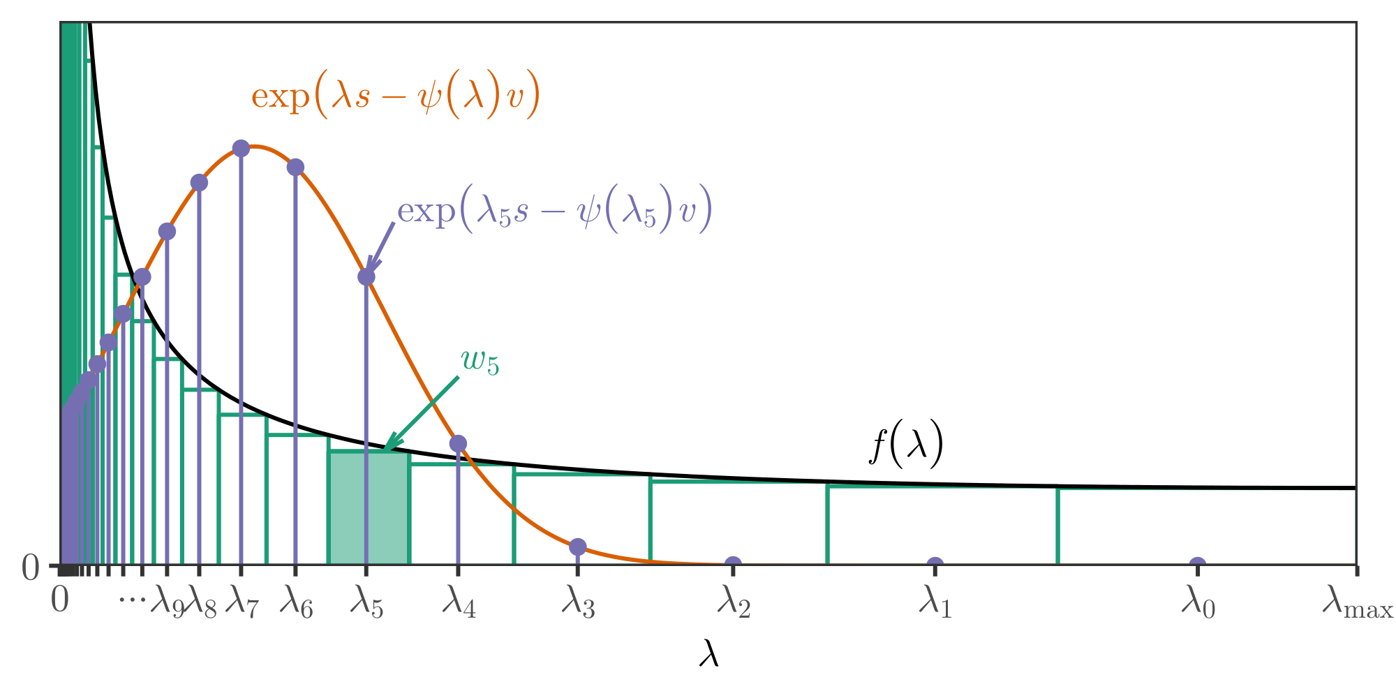
Recall the discrete mixture support points and weights,

$ \begin{align} \lambda_k \coloneqq \frac{\overline{\lambda}}{\eta^{k+1/2}} \quad \text{and} \quad w_k \coloneqq \frac{\overline{\lambda} (\eta - 1) f(\lambda_k\sqrt{\eta})}{\eta^{k+1}} \quad \text{for} \quad k = 0, 1, 2, \dots. \end{align} $

Figure 8 illustrates the construction. To see heuristically why the exponentially-spaced grid $\lambda_k = \mathcal{O}(\eta^{-k})$ makes sense, observe that the integrand $\exp \left\lbrace \lambda s - \lambda^2 v / 2 \right\rbrace$ is a scaled normal density in $\lambda$ with mean $s/v$ and standard deviation $1/\sqrt{v}$. In the regime relevant to our curved boundaries, $s$ is of order $\sqrt{v}$, ignoring logarithmic factors. Hence the integrand at time $v$ has both center and spread of order $1/\sqrt{v}$, so as $v \to \infty$, the relevant scale of the integrand shrinks. With the grid $\lambda_k = \mathcal{O}(\eta^{-k})$ we have $\lambda_k - \lambda_{k+1} = \mathcal{O}(\lambda_k)$, ensuring that the resolution of the grid around the peak of the integrand matches the scale of the integrand as $v \to \infty$.

The discrete mixture bound is a valid mixture boundary in its own right, based on a discrete mixing distribution, but we may wish to know how well it approximates the continuous-mixture boundary from which it is derived. To illustrate the accuracy of the discrete mixture construction, we compare it to the one-sided normal mixture bound, Proposition 21. By using the same half-normal mixing density in Theorem 9 and setting $\eta = 1.05$, $\overline{\lambda} = 100$, we may evaluate a corresponding discrete mixture bound $\textup{DM}\alpha$. With $\rho = 14.3$, $\alpha = 0.05$ and $l_0 = 1$, numerical calculations indicate that $\textup{DM}\alpha(v) / \textup{NM}_\alpha(v) \leq 1.004$ for $1 \leq v \leq 10^6$, suggesting that Theorem 9 gives an excellent conservative approximation to the corresponding continuous mixture boundary over a large practical range. Of course, when a closed form is available as in Proposition 21, one should use it in practice. But an exact closed form integral is rarely available as it is in Proposition 21, and substantial looseness often accompanies closed-form approximations which provably maintain crossing probability guarantees. In such cases, unless a closed form is required, Theorem 9 is preferable. See Figure 10 for an example; in this figure, the bounds of [19] and [24] involve closed-form mixture integral approximations.

Proof of Theorem 9: Because $f$ is nonincreasing, $f(\lambda) \geq f(\lambda_k \sqrt{\eta})$ on the interval $[\lambda_k / \sqrt{\eta}, \lambda_k \sqrt{\eta}]$, which has width $\lambda_{\max} (\eta - 1) / \eta^{k+1} = w_k / f(\lambda_k \sqrt{\eta})$. Hence $\sum_{k=0}^\infty w_k \leq \int_0^\infty f(\lambda) \mathop{}!\mathrm{d} \lambda = 1$. Let $G$ be a discrete distribution which places mass $w_k / \sum_{j=0}^\infty w_j$ at the point $\lambda_k$. By Lemma 7, we know the mixture bound $\mathcal{M}_\alpha$ applied to the discrete mixture distribution $G$ yields a sub- $\psi$ uniform boundary with crossing probability $\alpha$. But

$ \begin{align} \sum_{k=0}^\infty w_k \exp \left\lbrace \lambda_k s - \psi(\lambda_k) v \right\rbrace \leq \int \exp \left\lbrace \lambda s - \psi(\lambda) v \right\rbrace \mathop{}!\mathrm{d} G(\lambda), \end{align} $

so $\textup{DM}\alpha \geq \mathcal{M}\alpha$. That is, our discrete mixture approximation $\textup{DM}\alpha$ is a conservative overestimate of a corresponding exact mixture boundary $\mathcal{M}\alpha$, and can only have a lower crossing probability. So the discrete mixture bound $\textup{DM}\alpha$ satisfies the desired probability inequality $\mathbb{P}(\exists t : S_t \geq \textup{DM}\alpha(V_t)) \leq \alpha$.

A.6 Stitching as a discrete mixture approximation

Suppose we wish to analytically approximate the discrete mixture boundary $\textup{DM}_\alpha$ of Theorem 9 in the sub-Gaussian case $\psi = \psi_N$. Clearly the sum is lower bounded by the maximum summand, which gives

$ \begin{align} \textup{DM}\alpha(v) &\leq \sup\left\lbrace s \in \mathbb{R} : \sup{k \geq 0} \left[w_k \exp\left\lbrace \lambda_k s - \psi_N(\lambda_k) v \right\rbrace \right] < \frac{l_0}{\alpha} \right\rbrace \ &= \min_{k \geq 0} \left\lbrace \frac{\log(l_0 / w_k \alpha)}{\lambda_k} + \frac{\lambda_k}{2}, v \right\rbrace. \end{align} $

The last expression is the pointwise minimum of a collection of linear boundaries of the form presented in Lemma 4, each chosen with a different $\lambda_k$, and with nominal crossing rates $w_k \alpha$ so that a union bound over crossing events yields total crossing probability $\sum_k w_k \alpha \leq \alpha$. This is very similar to the stitching construction, with a slightly different choice of the sequence $\lambda_k$.

By equating $w_k$ from Theorem 9 with $1/h(k)$ from Theorem 5, this observation allows us to view a stitched bound with function $h(k)$ as an approximation to a mixture bound with mixture density $f(\lambda) = \Theta(1 / \lambda h(\log \lambda^{-1}))$ as $\lambda \downarrow 0$. For exponential stitching, this yields $f(\lambda) = \Theta(1)$ —densities approaching a nonzero constant as $\lambda \downarrow 0$, including the half-normal distribution, correspond to exponential stitched boundaries growing at a rate $\sqrt{V_t \log V_t}$. For polynomial stitching, we have the corresponding mixture density

$ \begin{align} f^{\text{LIL}}s(\lambda) \coloneqq \frac{(s - 1) s^{s-1} 1{0 \leq \lambda \leq \exp(-s)}} {\lambda \log^s \lambda^{-1}}, \end{align}\tag{41} $

matching the density from [19], Lemma 12 (we truncate at $\lambda = e^{-s}$ to ensure the density is nonincreasing). The "slower" function $h(k) \propto k \log^s k$ corresponds to $f(\lambda) = \Theta(1 / \lambda (\log \lambda^{-1}) (\log \log \lambda^{-1})^s)$, the density from example 3 of [22].

A.7 Proof of Theorem 10

The proof follows a straightforward idea. We break time into epochs $\eta^k \leq V_t < \eta^{k+1}$. Within each epoch we consider the linear boundary passing through the points $(\eta^k, g(\eta^k))$ and $(\eta^{k+1}, g(\eta^{k+1}))$. This line lies below $g(V_t)$ throughout the epoch, and its crossing probability is determined by its slope and intercept as in Lemma 4. Taking a union bound over epochs yields the result.

We need the following lemma concerning $g$:

########## {caption="Lemma 30"}

If $g$ is nonnegative and strictly concave on $\mathbb{R}_{\geq 0}$, then $g(v)$ is nondecreasing and $g(v) / v$ is strictly decreasing on $v > 0$.

Proof: If $s < 0$ is a supergradient of $g$ at some point $t$, then $g(t + u) < g(t) + s u < 0$ for sufficiently large $u$, contradicting the non-negativity of $g$. So $g$ is nondecreasing. Now fix $0 < x < y$ and let $s$ be any supergradient of $g$ at $x$. From nonnegativity and concavity we have $0 \leq g(0) \leq g(x) - x s$, so that $s \leq g(x) / x$. Strict concavity then implies $g(y) < g(x) + s (y - x) \leq g(x) y / x$.

Proof of Theorem 10: Fix any $\eta > 1$. On $\eta^k \leq v < \eta^{k+1}$ we lower bound $g(v)$ by the line $a_k + b_k v$ passing through the points $(\eta^k, g(\eta^k))$ and $(\eta^{k+1}, g(\eta^{k+1}))$. This line has intercept and slope

$ \begin{align} a_k &= \frac{\eta g(\eta^k) - g(\eta^{k+1})}{\eta - 1}, \ b_k &= \frac{g(\eta^{k+1}) - g(\eta^k)}{\eta^k (\eta - 1)}. \end{align} $

Note $a_k > 0$ and $b_k \geq 0$ by Lemma 30. We bound the upcrossing probability of this linear boundary using Lemma 4:

$ \begin{align} \mathbb{P}(\exists t \geq 1 : S_t \geq a_k + b_k V_t) \leq l_0 e^{-2 a_k b_k} = l_0 \exp \left\lbrace -\frac{2(g(\eta^{k+1}) - g(\eta^k))(\eta g(\eta^k) - g(\eta^{k+1}))} {\eta^k(\eta-1)^2} \right\rbrace. \end{align} $

The conclusion follows from a union bound over epochs and from the arbitrary choice of $\eta$.

Inspection of the proof reveals that the crossing probability bound Equation 14 is valid not only for the boundary $u$ given in Equation 13, but also for a similar boundary which is finite and linear for all $v < 1$ and $v > v_{\max}$. This follows by extending the linear boundaries over the first and last epochs.

A.8 Proof of Theorem 13

For the proof, we take $a = 0, b = 1$ without loss of generality. Write $Y_t \coloneqq X_t - \mathbb{E}{t-1} X_t$ and $\delta_t \coloneqq \widehat{X}t - \mathbb{E}{t-1} X_t$. Then $Y_t - \delta_t = X_t - \widehat{X}t \in [-1, 1]$. We will show that $\exp \left\lbrace \lambda \sum{i=1}^t Y_i - \psi_E(\lambda) \sum{i=1}^t (Y_i - \delta_i)^2 \right\rbrace$ is a supermartingale for each $\lambda \in [0, 1)$, where we take $c=1$ in $\psi_E$.

The proof of Lemma 4.1 in [81] shows that $\exp \left\lbrace \lambda \xi - \psi_E(\lambda) \xi^2 \right\rbrace \leq 1 + \lambda \xi$ for all $\lambda \in [0, 1)$ and $\xi \geq -1$. Applied to $\xi = y - \delta$, we have

$ \begin{align} \exp \left\lbrace \lambda y - \psi_E(\lambda)(y - \delta)^2 \right\rbrace \leq e^{\lambda \delta}(1 + \lambda (y - \delta)). \end{align} $

Since $Y_t - \delta_t \geq -1$, $\mathbb{E}_{t-1} Y_t = 0$, and $\delta_t$ is predictable, the above inequality implies

$ \begin{align} \mathbb{E}_{t-1} \exp \left\lbrace \lambda Y_t - \psi_E(\lambda)(Y_t - \delta_t)^2 \right\rbrace \leq e^{\lambda \delta_t}(1 - \lambda \delta_t) \leq 1, \end{align} $

using $1 - x \leq e^{-x}$ in the final step.

This shows that $S_t = \sum_{i=1}^t Y_i = \sum_{i=1}^t X_i - t \mu_t$ is sub-exponential with variance process $V_t = \sum_{i=1}^t (Y_i - \delta_i)^2 = \sum_{i=1}^t (X_i - \widehat{X}_i)^2$ and scale $c=1$. It follows that $\mathbb{P}(\exists t: S_t \geq u(V_t)) \leq \alpha$. A similar argument applied with $-X_t$ in place of $X_t$ shows that $\mathbb{P}(\exists t: -S_t \geq u(V_t)) \leq \alpha$, and a union bound finishes the proof. $\blacksquare$

We remark that the proofs of [17], Theorem 11, [18], Theorem 1, and [20] follow very different arguments. All three proofs involve a Bennett-type concentration bound for the sample mean with a radius depending on the true variance, combined via a union bound with a concentration bound for the sample variance. [18] and [20] achieve the latter bound using another Bennett/Bernstein-type inequality and the inequality $\mathbb{E} X^4 \leq \mathbb{E} X^2$ for $\lvert X\rvert \leq 1$, while [17] use a self-bounding property to achieve a concentration inequality for the sample variance directly ([17], Theorem 7).

In contrast, our argument avoids the union bound over the sample mean and sample variance bounds. We achieve this by constructing an exponential supermartingale which directly relates the deviations of $S_t$ to the "online" empirical variance $V_t$. In terms of proof technique, our method owes much more to the literature on self-normalized bounds ([82], [33], [83], [84] and especially [81]) than to the literature on empirical-Bernstein bounds.

A.9 Proof of Corollary 16

For case (1), Lemma 3(f) and Lemma 2 of [6] (cf. [84]) show that $S_t = \gamma_{\max}(Y_t)$ is sub-Gaussian with variance process $\widetilde{V}t = \gamma{\max}\left(\sum_{i=1}^t \frac{\Delta Y_i^2 + 2 \mathbb{E} \Delta Y_i^2}{3} \right)$. Invoking Corollary 6, we have

$ \begin{align} \limsup_{t \to \infty} \frac{S_t}{\sqrt{2 \widetilde{V}_t \log\log \widetilde{V}_t}} \leq 1 \quad \text{a.s. on } \left\lbrace \sup_t \widetilde{V}_t = \infty \right\rbrace. \end{align} $

Applying the strong law of large numbers elementwise, we have $t^{-1} \sum_{i=1}^t \frac{\Delta Y_i^2 + 2 \mathbb{E} \Delta Y_i^2}{3} \overset{a.s.}{\rightarrow} \mathbb{E} Y_1^2$ as $t \to \infty$, and the continuity of the maximum eigenvalue map over the set of positive semidefinite matrices ensures that $t^{-1} \widetilde{V}t \overset{\text{a.s.}}{\rightarrow} \gamma{\max}(\mathbb{E} Y_1^2) = t^{-1} V_t$. Hence, so long as $\mathbb{E} Y_1^2 > 0$ we conclude that, with probability one, $\sup_t \widetilde{V}_t = \infty$ and $\sqrt{\widetilde{V}_t \log \log \widetilde{V}t} \sim \sqrt{\gamma{\max}(\mathbb{E} Y_1^2) t \log \log t}$, completing the proof for case (1). (If $\mathbb{E} Y_1^2 = 0$ then the event $\lbrace \sup_t V_t = \infty \rbrace$ is empty and the result is vacuous.)

In case (2), Fact 1(d) and Lemma 2 of [6] (cf. [85]) show that $(S_t)$ defined as above is sub-gamma with variance process $(V_t)$ and scale $c$. The conclusion now follows directly from Corollary 6. $\blacksquare$

A.10 Proof of Corollary 17

The argument is adapted from [56]. Let $X_i \coloneqq x_i x_i^T - \Sigma$. The triangle inequality implies $\lVert X_i\rVert_{\text{op}} \leq \lVert x_i x_i^T\rVert_{\text{op}} + \lVert\Sigma\rVert_{\text{op}} \leq 2b$. Hence, by Fact 1(c) and Lemma 2 of [6] (cf. [85]), $S_t = \gamma_{\max}\left(\sum_{i=1}^t X_i \right)$ is sub-Poisson with scale $c = 2b$ and variance process

$ \begin{align} V_t &= \gamma_{\max}\left(\sum_{i=1}^t \mathbb{E} X_i^2 \right) \ &= \gamma_{\max} \left(\sum_{i=1}^t \left[\mathbb{E}[(x_i x_i^T)^2] - \Sigma^2 \right] \right) \ &\leq \sum_{i=1}^t \gamma_{\max}\left(\mathbb{E}[(x_i x_i^T)^2] \right). \end{align} $

In the final step, we neglect the negative semidefinite term $-\Sigma^2$ and use the fact that the maximum eigenvalue of a sum of positive semidefinite matrices is bounded by the sum of the maximum eigenvalues. We continue by using $\lVert x_i x_i^T\rVert = \lVert x_i\rVert_2^2 \leq b$ and the fact the expectation respects the semidefinite order to obtain

$ \begin{align} V_t &\leq \sum_{i=1}^t \gamma_{\max}\left(\mathbb{E} \lVert x_i\rVert_2^2 x_i x_i^T \right) \ &\leq t b \lVert\Sigma\rVert_{\text{op}}. \end{align} $

Plugging this upper bound on $V_t$ into the discrete mixture bound of Theorem 9 gives the result. $\blacksquare$

B. Implications among sub- $\psi$ boundaries

:Table 1: For each row, if $u$ is a sub- $\psi_1$ uniform boundary, subject to the given restriction, then $v \mapsto u(av)$ is a sub- $\psi_2$ uniform boundary. $\varphi(g, h)$ is defined in Equation 42. See Proposition 31 for details.

	$\psi_1$	$\psi_2$	$a$	Restriction
(1)	$\psi_N$	$\psi_{B, g, h}$	$\frac{\varphi(g, h)}{gh}$	any $g, h > 0$
(2)	$\psi_N$	$\psi_{B, g, h}$	$\frac{(g+h)^2}{4gh}$	any $g, h > 0$
(3)	$\psi_{P, c}$	$\psi_{B, g, g+c}$	1	any $g > -c$
(5)	$\psi_{G, c}$	$\psi_{P, 3c}$	1
(6)	$\psi_{E, c}$	$\psi_{G, 2c/3}$	1
(7)	$\psi_{G, c}$	$\psi_{E, c}$	1	$c \geq 0$
(8)	$\psi_{G, c}$	$\psi_{E, 2c}$	1	$c < 0$
(9)	$\psi_{P, c}$	$\psi_{G, c/2}$	1	$c < 0$
(10)	$\psi_N$	$\psi_{P, c}$	1	any $c < 0$
(11)	$\psi_{B, g, h}$	$\psi_{P, -g}$	1

Together with Table 1, the following proposition formalizes the relationships illustrated in Figure 2, restating Proposition 2 of [6] in the language of uniform boundaries. The first row of Table 1 uses the function

$ \begin{align} \varphi(g, h) \coloneqq \begin{cases} \frac{h^2 - g^2}{2 \log(h/g)}, & g < h \ gh, & g \geq h. \end{cases} \end{align}\tag{42} $

########## {caption="Proposition 31"}

For each row in Table 1, if $u$ is a sub- $\psi_1$ uniform boundary, and the given restrictions are satisfied, then $v \mapsto u(av)$ is a sub- $\psi_2$ uniform boundary for the given constant $a$. Furthermore, when we allow only transformations of the form $v \mapsto u(av)$, these capture all possible implications among the five sub- $\psi$ boundary types defined above, and the given constants are the best possible (in the case of row (2), the constant $(g+h)^2 / 4gh$ is the best possible of the form $k/gh$ where $k$ depends only on the total range $g + h$).

A reader who is familiar with [6] will note that the arrows in Figure 2 are reversed with respect to Figure 4 in their paper. Indeed, since any sub-Bernoulli process is also sub-Gaussian, it follows that any sub-Gaussian uniform boundary is also a sub-Bernoulli uniform boundary, and so on.

C. Additional proofs

C.1 Proof of Proposition 11

Let $k \coloneqq (l_0 / \alpha)^2$. For part (a), we will set the derivative of the squared objective $u^2(v) / v$ to zero:

$ \begin{align} \frac{\mathop{}!\mathrm{d}}{\mathop{}!\mathrm{d} v} \left[\left(1 + \frac{\rho}{v} \right)\left(\log\left(\frac{k(v+\rho)}{\rho} \right) \right) \right] = -\frac{\rho}{v^2} \log\left(\frac{k(v+\rho}{\rho} \right) + \frac{1}{v} &= 0 .\ -\left(\frac{v+\rho}{\rho} \right) \exp \left\lbrace -\frac{v+\rho}{\rho} \right\rbrace &= -\frac{1}{ek}. \end{align}\tag{43} $

We solve this equation using the lower branch $W_{-1}$ since we know $-(v+\rho)/\rho \leq -1$:

$ \begin{align} \frac{v+\rho}{\rho} &= -W_{-1}\left(-\frac{1}{ek} \right), \end{align} $

which is equivalent to 16.

For part (b), we optimize the squared boundary $u^2(v)$:

$ \begin{align} \frac{\mathop{}!\mathrm{d}}{\mathop{}!\mathrm{d} \rho} \left[(v + \rho) \log \left(\frac{k(v + \rho)}{\rho} \right) \right] = \log\left(\frac{k(v+\rho)}{\rho} \right) - \frac{v}{\rho} &= 0. \end{align} $

which is equivalent to 43. $\blacksquare$

C.2 Proof of Proposition 12

First, [26], Theorem 1 show that, for $B(t)$ a standard Brownian motion,

$ \begin{align} \mathbb{P}(\exists t \in (0, \infty) : B(t) \geq \mathcal{M}_\alpha(t)) = \alpha. \end{align}\tag{44} $

Let $(X_t){t=1}^\infty$ be any i.i.d. sequence of mean-zero random variables with unit variance and $\mathbb{E} e^{\lambda X_1} \leq e^{\lambda^2 / 2}$, for example standard normal or Rademacher random variables. For each $m \in \mathbb{N}$, let $S_t^{(m)} \coloneqq \sum{i=1}^t X_i / \sqrt{m}$ and $V_t^{(m)} \coloneqq t / m$, noting that $(S_t^{(m)})$ is sub-Gaussian with variance process $(V_t^{(m)})$. Our proof rests upon a standard application of Donsker's theorem, detailed below, which shows that, for any $T \in \mathbb{N}$,

$ \begin{align} \lim_{m \to \infty} \mathbb{P}\left(\exists t \in [mT] : S^{(m)}t \geq \mathcal{M}\alpha(V^{(m)}t) \right) = \mathbb{P}(\exists t \in (0, T] : B(t) \geq \mathcal{M}\alpha(t)). \end{align}\tag{45} $

To obtain the desired conclusion from Equation 45, we write, for any $m \in \mathbb{N}$ and $T \in \mathbb{N}$,

$ \begin{align} \mathbb{P}\left(\exists t \in \mathbb{N}: S_t^{(m)} \geq \mathcal{M}\alpha(V_t^{(m)}) \right) &\geq \mathbb{P}\left(\exists t \in [mT]: S_t^{(m)} \geq \mathcal{M}\alpha(V_t^{(m)}) \right). \end{align} $

Take $m \to \infty$ and use Equation 45 to find, for any $T \in \mathbb{N}$,

$ \begin{align} \liminf_{m \to \infty} \mathbb{P}\left(\exists t \in \mathbb{N}: S_t^{(m)} \geq \mathcal{M}\alpha(V_t^{(m)}) \right) &\geq \mathbb{P}\left(\exists t \in (0, T] : B(t) \geq \mathcal{M}\alpha(t) \right). \end{align} $

Now take $T \to \infty$ to obtain

$ \begin{align} \liminf_{m \to \infty} \mathbb{P}\left(\exists t \in \mathbb{N}: S_t^{(m)} \geq \mathcal{M}\alpha(V_t^{(m)}) \right) &\geq \mathbb{P}\left(\exists t \in (0, \infty) : B(t) \geq \mathcal{M}\alpha(t) \right) = \alpha, \end{align}\tag{46} $

by Equation 44. But for each $m \in \mathbb{N}$, $S_t^{(m)}$ is sub-Gaussian with variance process $V_t^{(m)}$, so that

$ \begin{align} \mathbb{P}\left(\exists t \in \mathbb{N}: S_t^{(m)} \geq \mathcal{M}_\alpha(V_t^{(m)}) \right) \leq \alpha. \end{align}\tag{47} $

Together, Equation 46 and 47 yield

$ \begin{align} \lim_{m \to \infty} \mathbb{P}\left(\exists t \in \mathbb{N}: S_t^{(m)} \geq \mathcal{M}_\alpha(V_t^{(m)}) \right) = \alpha. \end{align} $

Since $(S_t^{(m)}, V_t^{(m)}) \in \mathbb{S}_{\psi_N}^1$ for each $m$, the conclusion follows.

To prove Equation 45, we will use the fact that $\mathcal{M}\alpha: \mathbb{R}{\geq 0} \to \mathbb{R}{\geq 0}$ is continuous, increasing and concave, as proved in Lemma 32 below. For each $t \in \mathbb{R}{> 0}$ let $S(mt)$ be equal to $S_{mt}$ for $mt \in \mathbb{N}$ and a linear interpolation otherwise (with $S(0) = 0$). Let $C[0, T]$ denote the space of continuous, real-valued functions on $[0, T]$ equipped with the sup-norm, and let $\mathbb{P}_0$ denote the probability measure for standard Brownian motion. We first use a corollary of Donsker's theorem: for any $\varphi: C[0, T] \to \mathbb{R}$ continuous $\mathbb{P}_0$-a.s., we have ([77], Theorems 8.1.5, 8.1.11)

$ \begin{align} \varphi\left(\frac{S(m\cdot)}{\sqrt{m}} \right) \overset{\text{d}}{\rightarrow} \varphi(B(\cdot)) \quad \text{as } m \to \infty. \end{align} $

We let $\varphi(f) \coloneqq \sup_{t \in [0, T]} [f(t) - \mathcal{M}\alpha(t)]$, so that by compactness of $[0, T]$ and continuity of $f$ and $\mathcal{M}\alpha$, $\varphi(f) \geq 0$ if and only if $f(t) \geq \mathcal{M}\alpha(t)$ for some $t \in [0, T]$. Now $\varphi(S(m\cdot) / \sqrt{m}) \overset{\text{d}}{\rightarrow} \varphi(B(\cdot))$, and note that $\varphi(B(\cdot))$ has a continuous distribution: the distribution when $\mathcal{M}\alpha(t) \equiv 0$ is well-known by the reflection principle, and the measure for the Brownian motion with drift $B(t) - \mathcal{M}\alpha(t) + \mathcal{M}\alpha(0)$ is equivalent to the measure for $B(t)$ by the Cameron-Martin theorem ([86], Theorem 1.38). Hence

$ \begin{align} \mathbb{P}\left(\exists t \in [0, T] : \frac{S(mt)}{\sqrt{m}} \geq \mathcal{M}\alpha(t) \right) \to \mathbb{P}\left(\exists t \in [0, T] : B(t) \geq \mathcal{M}\alpha(t) \right). \end{align}\tag{48} $

But because $\mathcal{M}_\alpha(t)$ is concave, the linear interpolation of $S(\cdot)$ cannot add any new upcrossings beyond those in $(S_t)$:

$ \begin{align} \mathbb{P}\left(\exists t \in [0, T] : \frac{S(mt)}{\sqrt{m}} \geq \mathcal{M}\alpha(t) \right) &= \mathbb{P}\left(\exists x \in [mT] : \frac{S_x}{\sqrt{m}} \geq \mathcal{M}\alpha(x/m) \right) \ &= \mathbb{P}\left(\exists t \in [mT] : S^{(m)}t \geq \mathcal{M}\alpha(V^{(m)}_t) \right). \end{align}\tag{49} $

Combining Equation 49 with Equation 48 yields Equation 45, completing the proof. $\blacksquare$

########## {caption="Lemma 32"}

The function $\mathcal{M}\alpha: \mathbb{R}{\geq 0} \to \mathbb{R}_{\geq 0}$ is continuous, increasing and concave.

Proof: Continuity of $\mathcal{M}_\alpha(v)$ is clear from the continuity of $\exp \left\lbrace \lambda s - \psi(\lambda) v \right\rbrace$ in $s$ and $v$, which also implies

$ \begin{align} \int \exp \left\lbrace \lambda \mathcal{M}_\alpha(v) - \psi(\lambda) v \right\rbrace \mathop{}!\mathrm{d} F(\lambda) = \frac{l_0}{\alpha} \end{align} $

for all $v > 0$. That is, the left-hand side is constant in $v$, hence has derivative with respect to $v$ equal to zero. We may exchange the derivative and integral by Theorem A.5.1 of [77], noting that the integrand is positive and continuously differentiable in $v$ and $F$ is a probability measure. This yields

$ \begin{align} \mathcal{M}\alpha'(v) &= \frac{A(v)}{B(v)} > 0, \ \text{where } A(v) & \coloneqq \int \psi(\lambda) e^{\lambda \mathcal{M}\alpha(v) - \psi(\lambda) v} \mathop{}!\mathrm{d} F(\lambda) \ \text{and } B(v) & \coloneqq \int \lambda e^{\lambda \mathcal{M}_\alpha(v) - \psi(\lambda) v} \mathop{}!\mathrm{d} F(\lambda). \end{align} $

Both $A(v) > 0$ and $B(v) > 0$ since the integrands are positive, which shows that $\mathcal{M}_\alpha$ is increasing. Differentiating again yields, after some algebra,

$ \begin{align} B^2(v) \mathcal{M}\alpha''(v) &= \int \left(-\frac{[\lambda A(v) - \psi(\lambda) B(v)]^2}{B(v)} \right) e^{\lambda \mathcal{M}\alpha(v) - \psi(\lambda) v} \mathop{}!\mathrm{d} F(\lambda) \leq 0, \end{align} $

since the integrand is now nonpositive, showing that $\mathcal{M}_\alpha$ is concave.

C.3 Proof of Corollary 18

Write $\mu^\star \coloneqq \mathbb{E} T(X_1)$.We have noted in the discussion preceding the result that the exponential process $\exp \left\lbrace \lambda S_t(\mu) - t \psi_\mu(\lambda) \right\rbrace$ is the likelihood ratio testing $H_0: \theta = \theta(\mu)$ against $H_1: \theta = \theta(\mu) + \lambda$. It is well-known that the likelihood ratio is a martingale under the null. Hence $(S_t(\mu^\star))$ is sub- $\psi_{\mu^\star}$ with variance process $V_t = t$, and it follows immediately that $\mathbb{P}(\exists t: S_t(\mu^\star) \geq u_{\mu^\star}(t)) \leq \alpha_1$. Apply the same argument with $-X_t$ in place of $X_t$ to conclude that $\mathbb{P}(\exists t: -S_t(\mu^\star) \geq \tilde{u}_{\mu^\star}(t)) \leq \alpha_2$. A union bound completes the argument. $\blacksquare$

C.4 Proof of Lemma 19

The implication $(a) \Rightarrow (b)$ follows from

$ \begin{align} A_T &= \left[\bigcup_{t=1}^\infty A_t \cap \lbrace T = t \rbrace \right] \cup \left[A_\infty \cap \lbrace T = \infty \rbrace \right] \subseteq \bigcup_{t=1}^\infty A_t. \end{align} $

It is clear that $(b) \Rightarrow (c)$. For $(c) \Rightarrow (a)$, take $\tau = \inf\lbrace t \in \mathbb{N}: A_t \text{ occurs} \rbrace$, so that $A_\tau = \bigcup_{t = 1}^\infty A_t$. $\blacksquare$

D. Computing conjugate mixture bounds by root-finding

In this section we demonstrate that our conjugate mixture boundaries, which involve the supremum $\mathcal{M}_\alpha(v)$ defined in Equation 8, can be computed via root-finding. We assume that $\psi$ is CGF-like, a property which holds for all of the $\psi$ functions in Section 2:

########## {caption="Definition 33: [6], Definition 2"}

A real-valued function $\psi$ with domain $[0, \lambda_{\max})$ is called CGF-like if it is strictly convex and twice continuously differentiable with $\psi(0) = \psi'(0_+) = 0$ and $\sup_{\lambda \in [0, \lambda_{\max})} \psi(\lambda) = \infty$. For such a function, we write

$ \begin{align} \bar{b} \coloneqq \sup_{\lambda \in [0, \lambda_{\max})} \psi'(\lambda) \in (0, \infty]. \end{align} $

Lemma 7 implies that, with probability at least $1 - \alpha$, $m(S_t, V_t) < l_0 / \alpha$ for all $t$, where

$ \begin{align} m(s, v) &= \int \exp \left\lbrace \lambda s - \psi(\lambda) v \right\rbrace \mathop{}!\mathrm{d} F(\lambda). \end{align} $

We are interested in the set $A(v) \coloneqq \lbrace s \in \mathbb{R}: m(s, v) < l_0 / \alpha \rbrace$ for fixed $v \geq 0$. It is clear that $m(0, v) \leq 1 < l_0 / \alpha$ whenever $l_0 \geq 1$ (which holds in all cases we consider), since $\psi \geq 0$, $v \geq 0$ and $F$ is a probability distribution. So $0 \in A(v)$ always. We show below that, in addition, $A(v)$ is always an interval.

For one-sided boundaries, $F$ is supported on $\lambda \geq 0$, and so long as $F$ is not a point mass at zero (which would be an uninteresting mixture), $m(s, v)$ is strictly increasing in $s$ whenever $m(s, v) < \infty$. Hence $m(s, v) = l_0 / \alpha$ for at most one value of $s^\star(v) > 0$, in which case $A(v) = (-\infty, s^\star(v))$.

It is possible that $m(s, v) < l_0 / \alpha$ for all $s$ where the integral converges. To examine this case, we fix $v > 0$, which is the interesting case in practice, and make two observations:

• Whenever $s < \bar{b} v$, we have $m(s, v) < \infty$. Indeed, in this case, $\exp \left\lbrace \lambda s - \psi(\lambda) v \right\rbrace \to 0$ as $\lambda \to \infty$, and as the integrand is continuous in $\lambda$, it must be uniformly bounded. It follows immediately that we can have $m(s, v) = \infty$ only when $\bar{b} < \infty$.
• Whenever $\bar{b} < \infty$, we have $S_t \leq \bar{b} V_t$ a.s., a consequence of Theorem 1(a) of [6], which shows that $\mathbb{P}(\exists t: S_t \geq a + \bar{b} V_t) = 0$ for all $a > 0$. (To verify this fact, note we must have $\lambda_{\max} = \infty$ when $\bar{b} < \infty$ in order for the CGF-like condition $\sup_{\lambda \in [0, \lambda_{\max})} \psi(\lambda) = \infty$ to hold.)

Hence, when $\bar{b} = \infty$ we need not worry about $m(s, v) = \infty$. When $\bar{b} < \infty$, it suffices to check $m(\bar{b} v, v)$, which may be infinite. If $m(\bar{b} v, v) \geq l_0 / \alpha$, then we search for a root of $m(s, v) = l_0 / \alpha$ in the interval $s \in [0, \bar{b} v]$. If $m(\bar{b} v, v) < l_0 / \alpha$, it suffices to take $\mathcal{M}_\alpha(v) = \bar{b} v + \epsilon$ for any $\epsilon > 0$. In practice, it seems more reasonable to take the upper bound $\bar{b} v$ and use a closed confidence set instead of an open one.

For two-sided boundaries, when $F$ has support on both $\lambda > 0$ and $\lambda < 0$, in general we require the technical condition

$ \begin{align} \int \lvert\lambda\rvert^k \exp \left\lbrace \lambda s - \psi(\lambda) v \right\rbrace \mathop{}!\mathrm{d} F(\lambda) < \infty, \quad \text{for $k = 1, 2$.} \end{align}\tag{50} $

This ensures that we may differentiate $m(s, v)$ twice with respect to $s$, exchanging the derivative and the integral both times ([77], Theorem A.5.3). Hence, whenever condition Equation 50 holds,

$ \begin{align} \frac{\mathop{}!\mathrm{d}^2}{\mathop{}!\mathrm{d} s^2}, m(s, v) = \int \lambda^2 \exp \left\lbrace \lambda s - \psi(\lambda) v \right\rbrace \mathop{}!\mathrm{d} F(\lambda) \geq 0, \end{align} $

so that $m(s, v)$ is convex in $s$ for each $v \geq 0$. As $m(0, v) < l_0 / \alpha$, we conclude that $m(s, v) = l_0 / \alpha$ for at most one value $s^\star(v) > 0$ and one value $s_\star(v) < 0$, and $A(v) = (s_\star(v), s^\star(v))$. A similar discussion as above applies when $\bar{b} < \infty$ and we may have $m(s, v) = \infty$ for some values of $s$.

As Proposition 20 yields a closed-form result, only Proposition 22 requires that we verify condition Equation 50. From the proof of Proposition 22 in Appendix A.3, it suffices to show that

$ \begin{align} \int_0^1 \left\lvert\log\left(\frac{p}{1-p} \right)\right\rvert^k p^a (1 - p)^b \mathop{}!\mathrm{d} p < \infty \end{align} $

for some $a, b > 0$ and $k = 1, 2$. This follows from the fact that the integrand is continuous on $p \in (0, 1)$ and approaches zero as $p \to 0$ and $p \to 1$, so it is bounded.

E. Tuning discrete mixture implementation

In Section 3.5 we have discussed the choice of mixing precision in order to tune a mixture bound for a particular range of sample sizes. For discrete mixtures, the value $\overline{\lambda}$ must also be chosen, and this depends on the minimum relevant value of $V_t$: making $\overline{\lambda}$ larger will make the resulting bound tighter over smaller values of $V_t$ at the cost of a looser bound for larger values of $V_t$. In practice, for $\psi = \psi_G$, setting $\overline{\lambda} = [c + \sqrt{m / 2 \log \alpha^{-1}}]^{-1}$ will ensure the bound is tight for $V_t \geq m$. Furthermore, when evaluating $\textup{DM}\alpha(v)$ in practice, the sum can be truncated after $k{\max} = \lceil \log_\eta(\overline{\lambda} [c + \sqrt{5 v / \log \alpha^{-1}}]) \rceil$ terms. The remainder of this section explains these choices.

We wish to understand what range of values of $\lambda$ our discrete mixture must cover to ensure we get a tight bound for all $V_t \in [m, v_{\max}]$. At $V_t = m$ the value of $\lambda$ which yields the optimal linear bound from Lemma 4 is found by optimizing

$ \begin{align} \frac{\log \alpha^{-1}}{\lambda} + \frac{\psi(\lambda)}{\lambda} \cdot m, \end{align} $

yielding the first-order condition

$ \begin{align} \lambda \psi'(\lambda) - \psi(\lambda) = \frac{\log \alpha^{-1}}{m}. \end{align} $

For $\psi = \psi_G$, this becomes

$ \begin{align} \frac{\lambda^2}{2(1-c\lambda)^2} = \frac{\log \alpha^{-1}}{m}, \end{align} $

which is solved by

$ \begin{align} \lambda^\star(m) = \frac{1}{c + \sqrt{m / 2 \log \alpha^{-1}}}. \end{align} $

Large values of $\lambda$ are necessary to achieve tight bounds for small $V_t$. Hence, to ensure good performance at $V_t = m$ we choose $\overline{\lambda} = [c + \sqrt{m / 2 \log \alpha^{-1}}]^{-1}$. Similarly, to ensure the sum safely covers $V_t = v$ we ensure $\lambda_{k_{\max}} \leq [c + \sqrt{10 v / 2 \log \alpha^{-1}}]^{-1}$ (using an arbitrary "fudge factor" of ten), which yields $k_{\max} = \lceil \log_\eta(\lambda_{\max} [c + \sqrt{5 v / \log \alpha^{-1}}]) \rceil$.

We note that $\eta$ must also be chosen, but the only tradeoff here is computational. Smaller values of $\eta$ lead to more accurate approximations of the discrete mixture to the target continuous mixture, but require more terms to be summed. We have found $\eta = 1.1$ to provide excellent approximations in the examples we have examined.

F. Intrinsic time, change of units and minimum time conditions

In this section we point out that a bound expressed in terms of intrinsic time yields an infinite family of related bounds via scaling, and that "minimum time" conditions in such bounds (such as $m \vee V_t$ in Theorem 5) can be freely scaled as well. Suppose we have a uniform bound of the form

$ \begin{align} \mathbb{P}\left(\exists t \geq 1 : S_t \geq u_c(m \vee V_t) \right) \leq \alpha, \end{align}\tag{51} $

where intrinsic time $V_t$ has the same units as $S_t^2$, as usual, and $c$ is some parameter with the same units as $S_t$. Then, fixing any $\gamma > 0$ and applying the bound Equation 51 to the scaled observations $X_t / \sqrt{\gamma}$, which amounts to a change of units, we have

$ \begin{align} \alpha &\geq \mathbb{P}\left(\exists t \geq 1 : \frac{S_t}{\sqrt{\gamma}} \geq u_{c / \sqrt{\gamma}}\left(m \vee \frac{V_t}{\gamma} \right) \right) \ &= \mathbb{P}\left(\exists t \geq 1 : S_t \geq h_c(\gamma m \vee V_t) \right), \quad \text{where } h_c(v) \coloneqq \sqrt{\gamma} u_{c / \sqrt{\gamma}}\left(\frac{v}{\gamma} \right). \end{align} $

By changing units we have obtained a new bound on $S_t$ with different minimum time $\gamma m$ and a different shape. For example, applying this change of units to the stitched boundary Equation 4 with $m = 1$ yields the family of bounds

$ \begin{align} \mathbb{P}\left(\exists t \geq 1 : S_t \geq k_1 \sqrt{(\gamma \vee V_t)\ell\left(\frac{\gamma \vee V_t}{\gamma} \right)}

• c k_2 \ell\left(\frac{\gamma \vee V_t}{\gamma} \right) \right) \leq \alpha \end{align} $

for any $\gamma > 0$, with the definition of $\ell$ unchanged from Equation 4. Note only the argument of $\ell$ has been scaled. We started with a single bound Equation 4 expressed in terms of $V_t$ and ended up with a family of bounds on the same process $S_t$, one for each value of $\gamma$. Indeed, the tuning parameter $m$ in Theorem 5 is obtained by exactly this argument. The effect is more clear if we let $c = 0$ and examine the upper bound on the normalized process $S_t / \sqrt{V_t}$: then for any $\gamma > 0$, with probability at least $1 - \alpha$,

$ \begin{align} \frac{S_t}{\sqrt{V_t}} \leq \begin{cases} k_1 \sqrt{\ell\left(\frac{V_t}{\gamma} \right)}, & \text{when } V_t \geq \gamma, \ k_1 \sqrt{\frac{\gamma \ell(1)}{V_t}}, & \text{when } V_t < \gamma. \end{cases} \end{align} $

Now the right-hand depends on $V_t$ only through $V_t / \gamma$, so that the effect of changing $\gamma$ is simply to multiplicatively shift the bound backwards or forwards in time without changing the bounded process.

G. Detailed comparison of finite LIL bounds

Figure 9 and Figure 10 compare our finite LIL bounds to several existing bounds. Below we restate the original results from the various papers giving finite LIL bounds included in Figure 10. In Table 2, for ease of comparison, we write all bounds in the form

$ \begin{align} \mathbb{P}(\exists t \geq 1 : S_t \geq A \sqrt{t (\log \log B t + C)}, \end{align} $

valid for independent 1-sub-Gaussian observations. When the original bound holds only for $t \geq n$ instead of $t \geq 1$, we apply a change of units argument to replace $\log \log B t$ with $\log \log B n t$ and $t \geq n$ with $t \geq 1$, so that all bounds are comparable (see Appendix F). When bounds are expressed in terms of intrinsic time $V_t$ ([19]), this is formally justified. When they are expressed in terms of nominal time ([31, 24]) this is only a heuristic argument, but we conjecture that proofs of such bounds could be generalized to justify this scaling. When observations are i.i.d. from an infinitely divisible distribution, the change is formally justified by replacing each observation $X_i$ with a sum of $n$ i.i.d. "pseudo-observations" $Z_i$ such that $\sum_{i=1}^n Z_i \sim X_1$.

• [14], Lemma 1: for i.i.d. sub-Gaussian observations with variance parameter $\sigma^2$,

$ \begin{align} \mathbb{P}\left(\exists t \geq 1 : S_t \geq (1 + \sqrt{\epsilon}) \sqrt{ 2 \sigma^2 (1 + \epsilon) t \log\left(\frac{\log((1 + \epsilon) t)}{\delta} \right) } \right) \leq 1 - \frac{2 + \epsilon}{\epsilon} \left(\frac{\delta}{\log(1 + \epsilon)} \right)^{1 + \epsilon}. \end{align} $

• [13], Theorem 1: for sub-Gaussian observations with variance parameter $1/4$,

$ \begin{align} \mathbb{P}\left(\exists t \geq 1 : S_t \geq \sqrt{a t \log(\log_c t + 1) + b t} \right) \leq \zeta(2a / c) e^{-2b / c}. \end{align} $

• [12], Lemma 7: for independent sub-Gaussian observations with variance parameter $\sigma^2$,

$ \begin{align} \mathbb{P}\left(\exists t \geq 1 : S_t \geq \sqrt{2 \sigma^2 t (x + \eta \log \log(e t))} \right) \leq \sqrt{e} \zeta\left(\eta \left(1 - \frac{1}{2x} \right) \right) \left(\frac{\sqrt{x}}{2\sqrt{2}} + 1 \right)^\eta e^{-x} \end{align}\tag{52} $

• [19], Theorem 4: for $\lvert X_t\rvert \leq c_t$ a.s. and $V_t = \sum_{i=1}^t c_i^2$,

$ \begin{align} \mathbb{P}\left(\exists t \geq 1 : V_t \geq 173 \log\left(\frac{2}{\alpha} \right) : S_t \geq \sqrt{3 V_t (2 \log \log (3V_t / 2 S_t) + \log \alpha^{-1})} \right) \leq \alpha. \end{align} $

Though the bound is stated for bounded observations, the proof holds for any observations sub-Gaussian with variance parameters $(c_t^2)$, as noted in section 5.2 of [19]. Balsubramani suggests removing the initial time condition by imposing a constant bound over $t \leq 173 \log(2/\alpha)$ (section 5.3). We instead remove the condition by a change of units, as discussed in Appendix F.

• [31], eq. 22: for i.i.d. observations sub-Gaussian with variance parameter 1,

$ \begin{align} \mathbb{P}\left(\exists t \geq \eta^j : S_t \geq \frac{1 + \eta}{2 \sqrt{\eta}} \sqrt{t(2 c \log \log t - 2 c \log \log \eta + 2 \log a)} \right) \leq \frac{1}{a (c - 1)(j - 1/2)^{c - 1}}. \end{align} $

Darling and Robbins consider results for a general bound $\varphi(\lambda)$ on the moment-generating function of the observations. The result involves the term $h(v_t)$ where the function $h(\lambda) \coloneqq 1/2 + \lambda^{-2} \log \varphi(\lambda)$ and $v_t$ is unspecified but bounded.

• [24], eq. 2.2 and the example that follows: for i.i.d. observations sub-Gaussian with variance parameter 1,

$ \begin{align} \mathbb{P}\left(\exists t \geq 3 : S_t \geq A \sqrt{t(\log \log t + C)} \right) \leq \int_m^\infty \frac{A \sqrt{\log\log t + C}}{t} \exp \left\lbrace -\frac{A^2(\log\log t + C)}{2} \right\rbrace \mathop{}!\mathrm{d} t. \end{align}\tag{53} $

Darling and Robbins give a closed-form upper bound for the right-hand side of Equation 53. We instead evaluate it numerically, using readily-available implementations of the upper incomplete gamma function:

$ \begin{split} \int_m^\infty \frac{A \sqrt{\log\log t + C}}{t} \exp \left\lbrace -\frac{A^2(\log\log t + C)}{2} \right\rbrace \mathop{}!\mathrm{d} t \ = \frac{\sqrt{2\pi} A e^{-C}}{(A-2)^{3/2}}, \mathbb{P}\left(G \geq \frac{A^2 - 2}{2} (\log \log m + C) \right), \end{split} $

where $G \sim \Gamma(3/2, 1)$.

• Polynomial stitching as in Equation 6 with $c = 0$.
• Inverted stitching with $g(v) = A \sqrt{v (\log \log(e v) + C)}$ as in Equation 15. We set $v_{\max} = 10^{20}$ which covers 42 epochs with $\eta = 2.994$. To make for a fair comparison with polynomial stitching, observe that in 42 epochs with $s = 1.4$, polynomial stitching "spends" $\sum_{k=1}^{42} k^{-1.4} / \zeta(1.4) \approx 0.820$ of its crossing probability $\alpha$, so we run inverted stitching with $\alpha = 0.820 \cdot 0.025$.
• Normal mixture as in Equation 34 with $\rho \approx 0.13$:

$ \begin{align} u(v) \approx \sqrt{2 (v + 0.13) \log\left(20\sqrt{1+\frac{v}{0.13}} + 1 \right)}. \end{align} $

This is not a LIL boundary, so is not included in Table 2.

::: {caption="Table 2: Comparison of parameters $A, B, C$ for finite LIL boundaries expressed in the form ${\mathbb{P}(\exists t \geq 1 : S_t \geq A \sqrt{t (\log \log B t + C)}) \leq \alpha}$ for sums of independent 1-sub-Gaussian observations, with $\alpha = 0.025$. Functions $x(\alpha, \eta)$ and $C(\alpha, \dots)$ are given by numerical root-finding to set the corresponding error bound equal to $\alpha$."}

:::

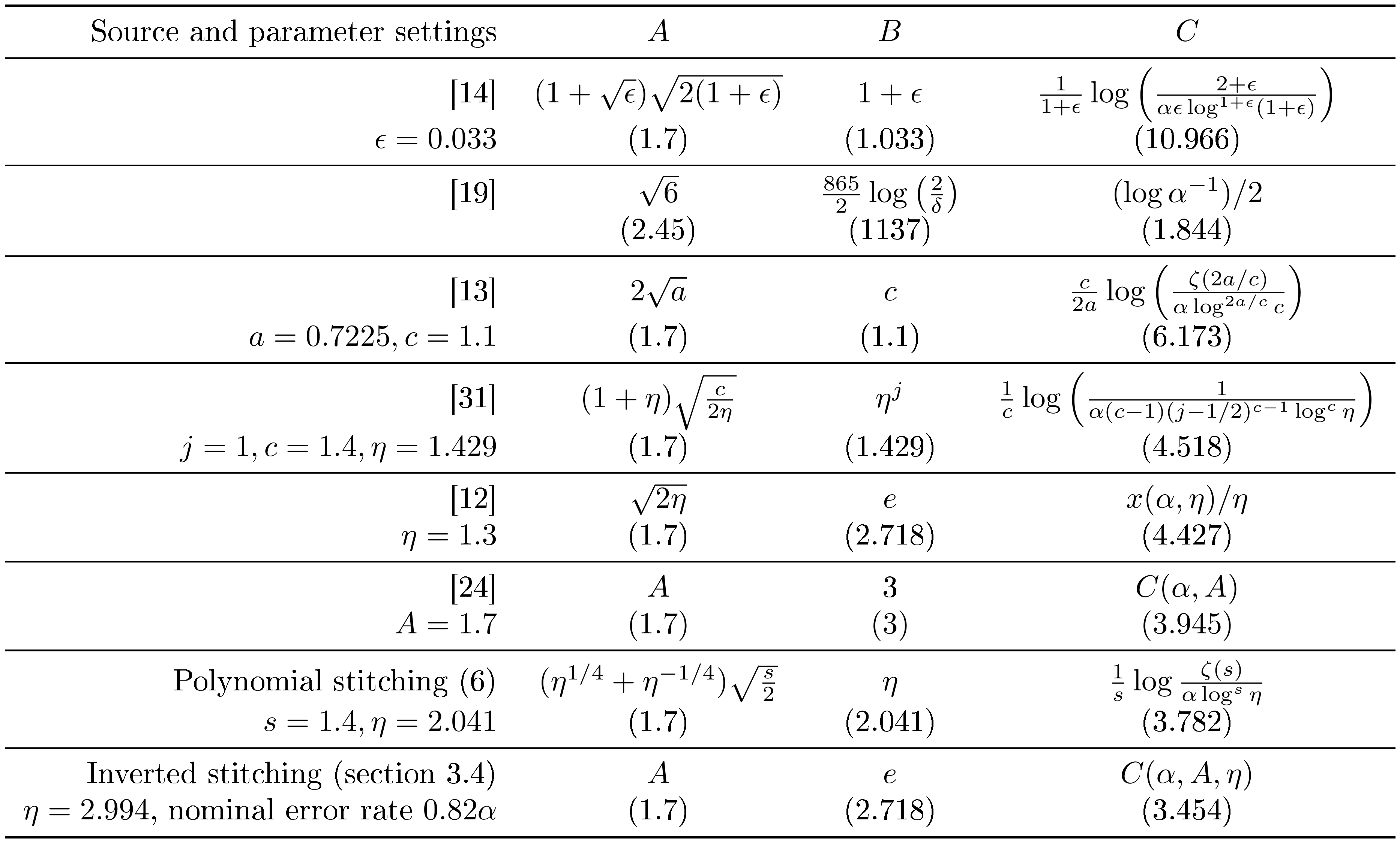
H. Details of Example 1

Write $X_t = \mu + \sigma Z_t$ for $t = 1, 2, \dots$ where $Z_1, Z_2, \dots$ are i.i.d. $\mathcal{N}(0, 1)$ random variables. Substituting into the definition of $S_t$, we find

$ \begin{align} S_t = \sum_{i=1}^{t+1} \left(Z_i - \bar{Z}_{t+1} \right)^2 - t, \end{align} $

where $\bar{Z}t \coloneqq t^{-1} \sum{i=1}^t Z_i$. Evidently the distribution of $S_t$ depends on neither $\mu$ nor $\sigma^2$. Furthermore, direct calculation shows that the increments of $(S_t)$ may be written as

$ \begin{align} \Delta S_t = S_t - S_{t-1} &= \frac{t}{t+1} \left(Z_{t+1} - \bar{Z}_t \right)^2 - 1\ & \eqqcolon Y_t^2 - 1, \end{align} $

where we define $Y_t \coloneqq \sqrt{t/(t+1)} (Z_{t+1} - \bar{Z}t)$ for $t = 1, 2, \dots$ (and take $S_0 = 0$ by convention). Noting that $Z{t+1} \sim \mathcal{N}(0, 1)$ is independent of $\bar{Z}_t \sim \mathcal{N}(0, t^{-1})$, we see that $Y_t \sim \mathcal{N}(0, 1)$ for each $t$. Finally, a straightforward calculation shows that $\mathbb{E} Y_i Y_j = 0$ for all $i \neq j$, so that $Y_1, Y_2, \dots$ are i.i.d. It follows that $\Delta S_1, \Delta S_2, \dots$ are i.i.d. centered Chi-squared random variables each with one degree of freedom. The CGF of this distribution is

$ \begin{align} \log \mathbb{E} e^{\lambda \Delta S_1} = -\frac{\log(1 - 2\lambda)}{2} - \lambda, \quad \text{for all } \lambda < \frac{1}{2}. \end{align}\tag{54} $

which is equal to $2 \psi_E(\lambda)$ with scale $c = 2$. As the increments of $(S_t)$ are i.i.d., it suffices for Definition 1 to have $\log \mathbb{E} e^{\lambda \Delta S_t} \leq \psi(\lambda) \Delta V_t$, and we have shown this holds with equality.

We have shown that $(S_t)$ is sub-exponential with scale $c = 2$ and variance process $V_t = 2t$. Recall that Definition 1 depends only on $\lambda \geq 0$. However, since Equation 54 holds for all $\lambda < 1/2$ and not just $0 \leq \lambda < 1/2$, replacing $\Delta S_t$ with $-\Delta S_t$ shows that $(-S_t)$ is sub-exponential with scale $c = -2$.

I. Extension to smooth Banach spaces and continuous-time processes

Though we have focused on discrete-time processes taking values in $\mathbb{R}$ or $\mathcal{S}^d$, our uniform boundaries also apply to discrete-time martingales in general smooth Banach spaces and to real-valued, continuous-time martingales. In this section we briefly review concepts from [6], Sections 3.4-3.5 to highlight the possibilities. First, let $(Y_t)_{t \in \mathbb{N}}$ be a martingale taking values in a separate Banach space $(\mathcal{X}, \lVert\cdot\rVert)$. Our uniform boundaries apply to any function $\Psi: \mathcal{X} \to \mathbb{R}$ satisfying the following property:

########## {caption="Definition: ([87])"}

A function $\Psi : \mathcal{X} \to \mathbb{R}$ is called $(2, D)$-smooth for some $D > 0$ if, for all $x, v \in \mathcal{X}$, we have (a) $\Psi(0) = 0$, (b) $\lvert\Psi(x + v) - \Psi(x)\rvert \leq \lVert v\rVert$, and (c) $\Psi^2(x + v) - 2 \Psi^2(x) + \Psi^2(x - v) \leq 2D^2 \lVert v\rVert^2$.

For example, the norm induced by the inner product in any Hilbert space is $(2, 1)$-smooth, and the Schatten $p$-norm is $(2, \sqrt{p-1})$-smooth for $p \geq 2$.

########## {caption="Corollary 34"}

Let $(Y_t){t \in \mathbb{N}}$ be a martingale taking values in a separable Banach space $(\mathcal{X}, \lVert\cdot\rVert)$, and $\Psi: \mathcal{X} \to \mathbb{R}$ is $(2, D)$-smooth; denote $D\star \coloneqq 1 \vee D$.

• (a) Suppose $\smash{\lVert\Delta Y_t\rVert \leq c_t}$ a.s. for all $t$ for constants $(c_t)$. Then, for any sub-Gaussian boundary $f$ with crossing probability $\alpha$ and $\smash{l_0 = 2}$, we have

$ \begin{align} \mathbb{P}\left(\exists t \geq 1: \Psi(Y_t) \geq f\left(D_\star^2 \sum_{i=1}^t c_i^2 \right) \right) \leq \alpha. \end{align} $

• (b) Suppose $\lVert\Delta Y_t\rVert \leq c$ a.s. for all $t$ for $\smash{c > 0}$. Then, for any sub-Poisson boundary $f$ with crossing probability $\alpha$, $l_0 = 2$, and scale $c$, we have

$ \begin{align} \mathbb{P}\left(\exists t \geq 1: \Psi(Y_t) \geq f\left(D_\star^2 \sum_{i=1}^t \mathbb{E}_{i-1} \lVert X_i\rVert^2 \right) \right) \leq \alpha. \end{align} $

The result follows directly from the proof of Corollary 10 in [6], which shows that $S_t = \Psi(Y_t)$ is sub-Gaussian or sub-Poisson with appropriate variance process $(V_t)$ for each case, building upon the work of [88, 87]. For example, let $(Y_t)$ be a martingale taking values in any Hilbert space, with $\lVert\cdot\rVert$ the induced norm, and suppose $\lVert\Delta Y_t\rVert \leq 1$ a.s. for all $t$. Then Corollary 34(a) with a normal mixture bound yields

$ \begin{align} \mathbb{P}\left(\exists t \geq 1: \lVert Y_t\rVert \geq \sqrt{(t + \rho) \log\left(\frac{4 (t + \rho)}{\alpha^2 \rho} \right)} \right) \leq \alpha. \end{align} $

Next, let $(S_t){t \in \mathbb{R}{\geq 0}}$ be a continuous-time, real-valued process. Replacing discrete-time processes in Definition 1 with continuous-time processes, and invoking the continuous-time version of Ville's inequality, our stitched, mixture and inverted stitching results extend straightforwardly to continuous time. Below we give two examples which follow from Fact 2 of [6]. Here $\left\langle S \right\rangle_t$ denotes the predictable quadratic variation of $(S_t)$.

########## {caption="Corollary 35"}

Let $(S_t){t \in \mathbb{R}{\geq 0}}$ be a real-valued process.

• (a) If $(S_t)$ is a locally square-integrable martingale with a.s. continuous paths, and $f$ is a sub-Gaussian stitched, mixture or inverted stitching uniform boundary, then $\mathbb{P}(\exists t \in (0, \infty): S_t \geq f(\left\langle S \right\rangle_t)) \leq e^{-2ab}$.
• (b) If $(S_t)$ is a local martingale with $\Delta S_t \leq c$ for all $t$, and $f$ is a sub-Poisson mixture bound for scale $c$ or a sub-gamma stitched bound for scale $c/3$, then $\mathbb{P}(\exists t \in (0, \infty): S_t \geq f(\left\langle S \right\rangle_t)) \leq \alpha$.

For example, if $(S_t)$ is a standard Brownian motion, then Corollary 35(a) with a polynomial stitched boundary yields, for any $\eta > 1, s > 1$,

$ \begin{align*} \mathbb{P}\left(\exists t \in (0, \infty): S_t \geq \frac{\eta^{1/4} + \eta^{-1/4}}{\sqrt{2}} \sqrt{ (1 \vee t) \left(s \log\log(\eta (1 \vee t))

• \log \frac{\zeta(s)}{\alpha \log^s \eta} \right) } \right) \leq \alpha. \end{align*} $

J. Sufficient conditions for Definition 1

Table 3 offers a summary of sufficient conditions for Definition 1 to hold when $(S_t)$ is a scalar process, while Table 4 gives conditions for matrix-valued processes. See [6], Section 2 for details.

::: {caption="Table 3: Summary of sufficient conditions a real-valued, discrete- or continuous-time process $(S_t)$ to be sub- $\psi$ with the given variance process. We assume $(S_t)$ is a martingale in every case except the starred ones ($^*$), when the first moment $\mathbb{E} \left\lvert X_t\right\rvert$ need not exist. See [6], Section 2 for details. One-sided conditions yield a bound on right-tail deviations only, while two-sided conditions yield bounds on both tails. For continuous-time cases, $\Delta S_t$ denotes the jumps of $(S_t)$ and $\left\langle S \right\rangle_t$ denotes the predictable quadratic variation. For the heavy on left case, the truncation function is defined as $T_a(y) \coloneqq (y \wedge a) \vee -a$ for $a > 0$ ([83]). The function $\varphi$ used in the Hoeffding-KS case is defined in Equation 42. The process $W_{m, t}$ in the continuous-time Bernstein case is defined in Fact 2(c) of [6] (cf. [89])."}

:::

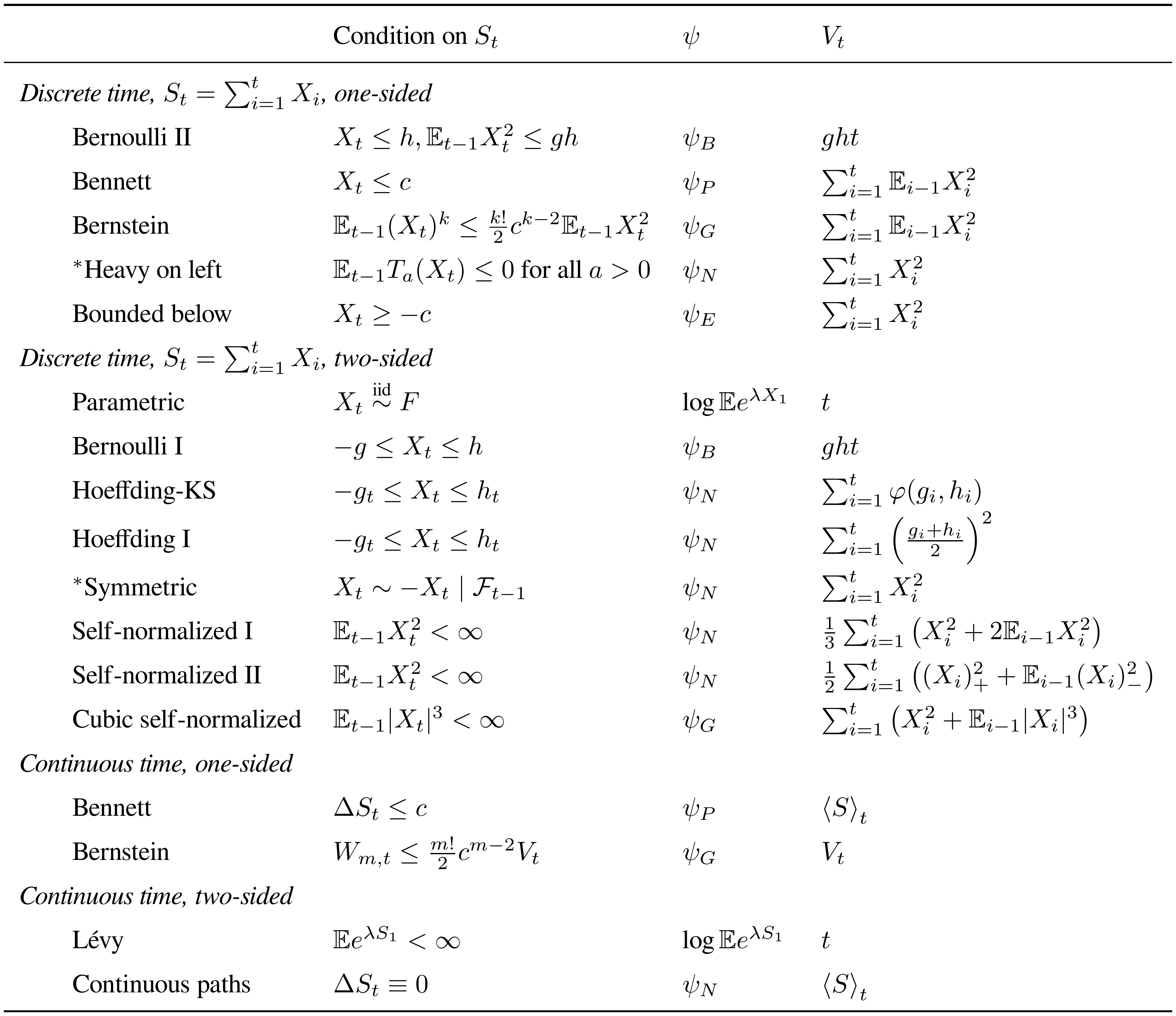
::: {caption="Table 4: Summary of sufficient conditions for Definition 1 when $Y_t = \sum_{i=1}^t X_i$ with $X_t \in \mathcal{H}^d$, the space of Hermitian, $d \times d$ matrices, taking $S_t = \gamma_{\max}(Y_t)$ and $V_t=\gamma_{\max}(Z_t)$. We assume $\mathbb{E} X_t = 0$ and hence $(Y_t)$ is a martingale in every case except the symmetric$^*$ case, when the first moment $\mathbb{E} \lvert X_t\rvert$ need not exist. See [6], Section 2 for details. One-sided conditions yield a bound on right-tail deviations only, while two-sided conditions yields bounds on both tails. The function $\varphi$ used in the Hoeffding-KS case is defined in Equation 42."}

:::

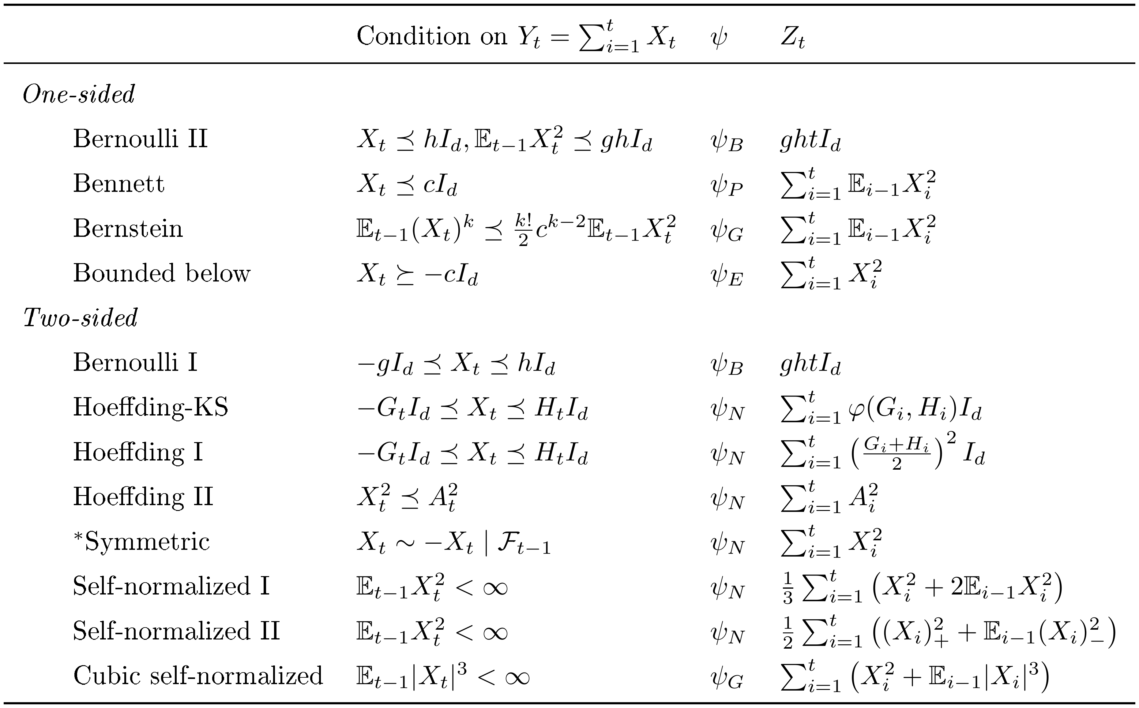
References

[1] Armitage, P., McPherson, C. K. and Rowe, B. C. 1969, 'Repeated significance tests on accumulating data', Journal of the Royal Stat. Society, Series A132(2), 235–244.

[2] Berman, R., Pekelis, L., Scott, A. and Van den Bulte, C. 2018, p-hacking and false discovery in A/B testing, Technical Report 3204791, SSRN.

[3] Darling, D. A. and Robbins, H. 1967a, 'Confidence Sequences for Mean, Variance, and Median', Proceedings of the National Academy of Sciences58(1), 66–68.

[4] Lai, T. L. 1984, 'Incorporating scientific, ethical and economic considerations into the design of clinical trials in the pharmaceutical industry: a sequential approach', Communications in Statistics - Theory and Methods13(19), 2355–2368.

[5] Jennison, C. and Turnbull, B. W. 1989, 'Interim Analyses: The Repeated Confidence Interval Approach', Journal of the Royal Statistical Society, Series B51(3), 305–361.

[6] Howard, S. R., Ramdas, A., McAuliffe, J. and Sekhon, J. 2020, 'Time-uniform Chernoff bounds via nonnegative supermartingales', Probability Surveys17, 257–317.

[7] Jamieson, K., Malloy, M., Nowak, R. and Bubeck, S. 2014, lil' UCB: An Optimal Exploration Algorithm for Multi-Armed Bandits, in'Proceedings of The 27th Conference on Learning Theory', Vol. 35, pp. 423–439.

[8] Jennison, C. and Turnbull, B. W. 1984, 'Repeated confidence intervals for group sequential clinical trials', Controlled Clinical Trials5(1), 33–45.

[9] Johari, R., Pekelis, L. and Walsh, D. J. 2015, 'Always valid inference: Bringing sequential analysis to A/B testing', arXiv preprint arXiv:1512.04922.

[10] Jamieson, K. and Jain, L. 2018, A bandit approach to multiple testing with false discovery control, in'Proceedings of the 32nd International Conference on Neural Information Processing Systems', pp. 3664–3674.

[11] Garivier, A. 2013, Informational confidence bounds for self-normalized averages and applications, in'2013 IEEE Information Theory Workshop (ITW)', IEEE, pp. 1–5.

[12] Kaufmann, E., Cappé, O. and Garivier, A. 2016, 'On the complexity of best-arm identification in multi-armed bandit models', The Journal of Machine Learning Research17(1), 1–42.

[13] Zhao, S., Zhou, E., Sabharwal, A. and Ermon, S. 2016, Adaptive concentration inequalities for sequential decision problems, in'30th Conference on Neural Information Processing Systems'.

[14] Jamieson, K. and Nowak, R. 2014, Best-arm identification algorithms for multi-armed bandits in the fixed confidence setting, in'48th Annual Conference on Information Sciences and Systems (CISS)', pp. 1–6.

[15] Yang, F., Ramdas, A., Jamieson, K. G. and Wainwright, M. J. 2017, A framework for Multi-A(rmed)/B(andit) testing with online FDR control, in'31st Conference on Neural Information Processing Systems'.

[16] Malek, A., Katariya, S., Chow, Y. and Ghavamzadeh, M. 2017, Sequential multiple hypothesis testing with Type I error control, in'Artificial Intelligence and Statistics', pp. 1468–1476.

[17] Maurer, A. and Pontil, M. 2009, Empirical Bernstein bounds and sample variance penalization, in'Proceedings of the Conference on Learning Theory'.

[18] Audibert, J.-Y., Munos, R. and Szepesvári, C. 2009, 'Exploration–exploitation tradeoff using variance estimates in multi-armed bandits', Theoretical Computer Science410(19), 1876–1902.

[19] Balsubramani, A. 2014, 'Sharp Finite-Time Iterated-Logarithm Martingale Concentration', arXiv:1405.2639.

[20] Balsubramani, A. and Ramdas, A. 2016, Sequential Nonparametric Testing with the Law of the Iterated Logarithm, in'Proceedings of the Thirty-Second Conference on Uncertainty in Artificial Intelligence', UAI'16, AUAI Press, pp. 42–51.

[21] Wald, A. 1945, 'Sequential Tests of Statistical Hypotheses', Annals of Mathematical Statistics16(2), 117–186.

[22] Robbins, H. 1970, 'Statistical Methods Related to the Law of the Iterated Logarithm', The Annals of Mathematical Statistics41(5), 1397–1409.

[23] Ville, J. 1939, Étude Critique de la Notion de Collectif., Gauthier-Villars, Paris.

[24] Darling, D. A. and Robbins, H. 1968, 'Some Further Remarks on Inequalities for Sample Sums', Proceedings of the National Academy of Sciences60(4), 1175–1182.

[25] Robbins, H. and Siegmund, D. 1969, 'Probability Distributions Related to the Law of the Iterated Logarithm', Proc. of the National Academy of Sciences62(1), 11–13.

[26] Robbins, H. and Siegmund, D. 1970, 'Boundary crossing probabilities for the Wiener process and sample sums', The Annals of Mathematical Statistics41(5), 1410–1429.

[27] Lai, T. L. 1976b, 'On Confidence Sequences', The Annals of Statistics4(2), 265–280.

[28] de la Peña, V. H., Klass, M. J. and Lai, T. L. 2007, 'Pseudo-maximization and self-normalized processes', Probability Surveys4, 172–192.

[29] Bercu, B., Delyon, B. and Rio, E. 2015, Concentration Inequalities for Sums and Martingales, Springer International Publishing, Cham.

[30] Kaufmann, E. and Koolen, W. 2018, 'Mixture martingales revisited with applications to sequential tests and confidence intervals', arXiv:1811.11419.

[31] Darling, D. A. and Robbins, H. 1967b, 'Iterated Logarithm Inequalities', Proceedings of the National Academy of Sciences57(5), 1188–1192.

[32] Robbins, H. and Siegmund, D. 1968, Iterated logarithm inequalities and related statistical procedures, in'Mathematics of the Decision Sciences, Part II', American Mathematical Society, Providence, pp. 267–279.

[33] de la Peña, V. H., Klass, M. J. and Lai, T. L. 2004, 'Self-normalized processes: exponential inequalities, moment bounds and iterated logarithm laws', The Annals of Probability32(3), 1902–1933.

[34] de la Peña, V. H., Klass, M. J. and Lai, T. L. 2009, 'Theory and applications of multivariate self-normalized processes', Stochastic Processes and their Applications119(12), 4210–4227.

[35] de la Peña, V. H., Lai, T. L. and Shao, Q.-M. 2009, Self-normalized processes: limit theory and statistical applications, Springer, Berlin.

[36] Johari, R., Koomen, P., Pekelis, L. and Walsh, D. 2017, Peeking at A/B Tests: Why it matters, and what to do about it, ACM Press, pp. 1517–1525.

[37] Hoeffding, W. 1963, 'Probability Inequalities for Sums of Bounded Random Variables', Journal of the American Statistical Association58(301), 13–30.

[38] Azuma, K. 1967, 'Weighted sums of certain dependent random variables.', Tohoku Mathematical Journal19(3), 357–367.

[39] McDiarmid, C. 1998, Concentration, inM. Habib, C. McDiarmid, J. Ramirez-Alfonsin and B. Reed, eds, 'Probabilistic Methods for Algorithmic Discrete Mathematics', Springer, New York, pp. 195–248.

[40] Raginsky, M., Sason, I. et al. 2013, 'Concentration of measure inequalities in information theory, communications, and coding', Foundations and Trends in Communications and Information Theory10(1-2), 1–246.

[41] Cramér, H. 1938, 'Sur un nouveau théorème-limite de la théorie des probabilités', Actualités Scientifiques736.

[42] Chernoff, H. 1952, 'A measure of asymptotic efficiency for tests of a hypothesis based on the sum of observations', The Annals of Mathematical Statistics23(4), 493–507.

[43] Boucheron, S., Lugosi, G. and Massart, P. 2013, Concentration inequalities: a nonasymptotic theory of independence, 1st edn, Oxford University Press, Oxford.

[44] Jorgensen, B. 1997, The Theory of Dispersion Models, CRC Press.

[45] Stout, W. F. 1970, 'The Hartman-Wintner Law of the Iterated Logarithm for Martingales', Annals of Mathematical Statistics41(6), 2158–2160.

[46] Lai, T. L. 1976a, 'Boundary Crossing Probabilities for Sample Sums and Confidence Sequences', The Annals of Probability4(2), 299–312.

[47] Neyman, J. 1923/1990, 'On the Application of Probability Theory to Agricultural Experiments, Essay on Principles, Section 9', Statistical Science5(4), 465–480.

[48] Rubin, D. B. 1974, 'Estimating causal effects of treatments in randomized and nonrandomized studies.', Journal of educational Psychology66(5), 688.

[49] Imbens, G. W. and Rubin, D. B. 2015, Causal Inference for Statistics, Social, and Biomedical Sciences: An Introduction, 1 edn, Cambridge University Press.

[50] Efron, B. 1971, 'Forcing a sequential experiment to be balanced', Biometrika58(3), 403–417.

[51] Aronow, P. M. and Middleton, J. A. 2013, 'A class of unbiased estimators of the average treatment effect in randomized experiments', Journal of Causal Inference1(1), 135–154.

[52] Tropp, J. A. 2011, 'Freedman's inequality for matrix martingales', Electronic Communications in Probability16, 262–270.

[53] Rudelson, M. 1999, 'Random Vectors in the Isotropic Position', Journal of Functional Analysis164(1), 60–72.

[54] Vershynin, R. 2012, Introduction to the non-asymptotic analysis of random matrices, in'Compressed Sensing: Theory and Applications', Cambridge University Press.

[55] Gittens, A. and Tropp, J. A. 2011, 'Tail bounds for all eigenvalues of a sum of random matrices', ACM Report 2014-02, Caltech.

[56] Tropp, J. A. 2015, 'An Introduction to Matrix Concentration Inequalities', Foundations and Trends in Machine Learning8(1-2), 1–230.

[57] Koltchinskii, V. and Lounici, K. 2017, 'Concentration inequalities and moment bounds for sample covariance operators', Bernoulli23(1), 110–133.

[58] Robbins, H. and Siegmund, D. 1972, A class of stopping rules for testing parametric hypotheses, The Regents of the University of California.

[59] Robbins, H. and Siegmund, D. 1974, 'The Expected Sample Size of Some Tests of Power One', The Annals of Statistics2(3), 415–436.

[60] Wald, A. 1947, Sequential Analysis, John Wiley & Sons, New York.

[61] Lorden, G. and Pollak, M. 2005, 'Nonanticipating estimation applied to sequential analysis and changepoint detection', The Annals of Statistics33(3), 1422–1454.

[62] Siegmund, D. and Gregory, P. 1980, 'A Sequential Clinical Trial for Testing $p_1 = p_2

#39;, The Annals of Statistics8(6), 1219–1228.

[63] Lai, T. L. 1997, 'On optimal stopping problems in sequential hypothesis testing', Statistica Sinica7(1), 33–51.

[64] Kulldorff, M., Davis, R. L., Kolczak†, M., Lewis, E., Lieu, T. and Platt, R. 2011, 'A Maximized Sequential Probability Ratio Test for Drug and Vaccine Safety Surveillance', Sequential Analysis30(1), 58–78.

[65] Shafer, G., Shen, A., Vereshchagin, N. and Vovk, V. 2011, 'Test Martingales, Bayes Factors and p-Values', Statistical Science26(1), 84–101.

[66] Grünwald, P., de Heide, R. and Koolen, W. 2019, 'Safe testing', arXiv:1906.07801.

[67] Pocock, S. J. 1977, 'Group Sequential Methods in the Design and Analysis of Clinical Trials', Biometrika64(2), 191–199.

[68] O'Brien, P. C. and Fleming, T. R. 1979, 'A Multiple Testing Procedure for Clinical Trials', Biometrics35(3), 549–556.

[69] Lan, K. K. G. and DeMets, D. L. 1983, 'Discrete Sequential Boundaries for Clinical Trials', Biometrika70(3), 659–663.

[70] Jennison, C. and Turnbull, B. W. 2000, Group sequential methods with applications to clinical trials, Chapman & Hall/CRC, Boca Raton.

[71] Siegmund, D. 1978, 'Estimation Following Sequential Tests', Biometrika65(2), 341.

[72] Garivier, A. and Leonardi, F. 2011, 'Context tree selection: A unifying view', Stochastic Processes and their Applications121(11), 2488–2506.

[73] Lai, T. L. and Siegmund, D. 1977, 'A Nonlinear Renewal Theory with Applications to Sequential Analysis I', The Annals of Statistics5(5), 946–954.

[74] Lai, T. L. and Siegmund, D. 1979, 'A Nonlinear Renewal Theory with Applications to Sequential Analysis II', The Annals of Statistics7(1), 60–76.

[75] Siegmund, D. 1985, Sequential Analysis, Springer New York, New York, NY.

[76] Whitehead, J. and Stratton, I. 1983, 'Group Sequential Clinical Trials with Triangular Continuation Regions', Biometrics39(1), 227–236.

[77] Durrett, R. 2017, Probability: Theory and Examples, 5a edn.

[78] Freedman, D. A. 1975, 'On Tail Probabilities for Martingales', The Annals of Probability3(1), 100–118.

[79] Widder, D. V. 1942, Laplace Transform, Princeton University Press, Princeton.

[80] Fulks, W. 1951, 'A Generalization of Laplace's Method', Proceedings of the American Mathematical Society2(4), 613–622.

[81] Fan, X., Grama, I. and Liu, Q. 2015, 'Exponential inequalities for martingales with applications', Electronic Journal of Probability20(1), 1–22.

[82] de la Peña, V. H. 1999, 'A General Class of Exponential Inequalities for Martingales and Ratios', The Annals of Probability27(1), 537–564.

[83] Bercu, B. and Touati, A. 2008, 'Exponential inequalities for self-normalized martingales with applications', The Annals of Applied Probability18(5), 1848–1869.

[84] Delyon, B. 2009, 'Exponential inequalities for sums of weakly dependent variables', Electronic Journal of Probability14, 752–779.

[85] Tropp, J. A. 2012, 'User-friendly tail bounds for sums of random matrices', Foundations of Computational Mathematics12(4), 389–434.

[86] Morters, P. and Peres, Y. 2010, Brownian Motion, Cambridge University Press, Cambridge.

[87] Pinelis, I. 1994, 'Optimum Bounds for the Distributions of Martingales in Banach Spaces', The Annals of Probability22(4), 1679–1706.

[88] Pinelis, I. 1992, An Approach to Inequalities for the Distributions of Infinite-Dimensional Martingales, in'Probability in Banach Spaces, 8: Proceedings of the Eighth International Conference', Birkhäuser, Boston, MA, pp. 128–134.

[89] van de Geer, S. 1995, 'Exponential Inequalities for Martingales, with Application to Maximum Likelihood Estimation for Counting Processes', The Annals of Statistics23(5), 1779–1801.