KPConv: Flexible and Deformable Convolution for Point Clouds

Hugues ThomasCharles R. QiJean-Emmanuel DeschaudBeatriz MarcoteguiFrançois GouletteLeonidas J. Guibas

article2019ICCV3,449 citations

Proposes Kernel Point Convolution (KPConv), a convolution operator that learns continuous and deformable kernel point locations directly on raw 3D point clouds, enabling networks to adapt to complex geometries and varying densities without intermediate grid representations.

Listen

The paper introduces Kernel Point Convolution (KPConv), a convolution operator designed to process 3D point clouds directly without projecting them onto grids or other intermediate structures. Point clouds from scanning technologies are sparse, unordered, and unevenly dense, which prevents standard image-style convolutions from working efficiently. The work addresses the resulting performance gaps in classification and segmentation by defining kernel weights through a small set of kernel points placed in continuous Euclidean space and correlated with nearby input points via a simple linear function.

The authors set out to create a flexible point convolution that supports both fixed and learned kernel shapes while remaining computationally efficient. They implemented rigid KPConv with regularly spaced kernel points and a deformable version that predicts local shifts to adapt kernels to scene geometry. Both versions use radius neighborhoods and grid-based subsampling to maintain robustness across density variations. The resulting KP-CNN and KP-FCNN architectures were evaluated on ModelNet40 for classification and on ShapeNetPart, ScanNet, S3DIS, Semantic3D, and Paris-Lille-3D for segmentation, with comparisons against prior point-based and projection-based methods.

Rigid KPConv achieved the highest overall accuracy on ModelNet40 (92.9 percent) and competitive results on simpler segmentation tasks, while the deformable version delivered the best scores on the larger, more diverse scene datasets, reaching 67.1 percent mean intersection-over-union on S3DIS Area 5 and 75.9 percent on Paris-Lille-3D. Deformable kernels proved more robust when the number of kernel points was reduced and produced effective receptive fields that better matched object scale and structure. Both variants trained and ran at practical speeds on consumer GPUs while using roughly 14–15 million parameters.

These outcomes indicate that explicit spatial kernels located by points can surpass MLP-based or graph-based alternatives in accuracy without added complexity. The gains matter most for applications that require reliable 3D scene understanding from raw scans, such as robotics, autonomous driving, and infrastructure modeling. Rigid kernels suffice for smaller or less varied data, whereas deformable kernels become advantageous once object diversity and scene scale increase.

The authors recommend selecting the rigid or deformable form according to task complexity and dataset size, and they release their code to support further work. They note that deformable convolutions are likely to scale well to larger collections or new tasks such as object detection and point-cloud completion. The main limitations are that results were obtained on six specific benchmarks and that the deformable variant requires an auxiliary regularization loss to keep kernel points aligned with input geometry; performance on even larger or noisier real-world data therefore remains to be confirmed.

École des Mines de Paris Meta Stanford University classification fast fourier transforms local geometry Kernel Point Convolution point cloud deformable convolution

arXiv: 1904.08889 HuguesTHOMAS/KPConv

Paper: PointNet: Deep Learning on Point Sets for 3D Classification and Segmentation, Charles R. Qi et al. (2017). Reading PointNet is essential because it introduces the foundational architecture for processing unordered point sets directly, establishing the core paradigm that KPConv builds upon.
Paper: PointNet++: Deep Hierarchical Feature Learning on Point Sets in a Metric Space, C. Qi et al. (2017). PointNet++ provides the crucial background on hierarchical metric-space feature learning and local neighborhood aggregation that directly motivates KPConv's continuous spatial convolution design.
Paper: Deformable Convolutional Networks, Jifeng Dai et al. (2017). This paper establishes the mechanism of deformable convolutions on regular image grids, which is a conceptual prerequisite for understanding KPConv's extension to deformable point convolutions.
Paper: Dynamic Graph CNN for Learning on Point Clouds, Yue Wang et al. (2018). Dynamic Graph CNN introduces graph-based local neighborhood operations for point clouds, offering important comparative context for KPConv's Euclidean-space kernel point approach.
Paper: Geometric Deep Learning: Going beyond Euclidean data, Michael M. Bronstein et al. (2016). This survey on geometric deep learning provides the theoretical taxonomy needed to understand how point cloud convolutions fit into the broader landscape of non-Euclidean data processing.

Paper: Fast Graph Representation Learning with PyTorch Geometric, Matthias Fey et al. (2019). PyTorch Geometric builds directly on foundational point and graph operators like KPConv by providing a unified software library for high-throughput GPU implementation.

Cover for KPConv: Flexible and Deformable Convolution for Point Clouds

Abstract

We present Kernel Point Convolution (KPConv), a new design of point convolution, i.e. that operates on point clouds without any intermediate representation. The convolution weights of KPConv are located in Euclidean space by kernel points, and applied to the input points close to them. Its capacity to use any number of kernel points gives KPConv more flexibility than fixed grid convolutions. Furthermore, these locations are continuous in space and can be learned by the network. Therefore, KPConv can be extended to deformable convolutions that learn to adapt kernel points to local geometry. Thanks to a regular subsampling strategy, KPConv is also efficient and robust to varying densities. Whether they use deformable KPConv for complex tasks, or rigid KPconv for simpler tasks, our networks outperform state-of-the-art classification and segmentation approaches on several datasets. We also offer ablation studies and visualizations to provide understanding of what has been learned by KPConv and to validate the descriptive power of deformable KPConv.

Topics

classification fast fourier transforms local geometry point cloud visualization intermediate representations

Keywords

Kernel Point Convolution point cloud deformable convolution radius neighborhood regular subsampling effective receptive field rigid KPConv segmentation classification kernel point initialization

1. Introduction
2. Related Work
3. Kernel Point Convolution
3.1. A Kernel Function Defined by Points
3.2. Rigid or Deformable Kernel
3.3. Kernel Point Network Layers
3.4. Kernel Point Network Architectures
4. Experiments
4.1. 3D Shape Classification and Segmentation
4.2. 3D Scene Segmentation
4.3. Ablation Study
4.4. Learned Features and Effective Receptive Field
5. Conclusion
References
A. Network Architectures and Parameters
B. Kernel Points Initialization
C. Effect of the Kernel Point Regularization
D. More Segmentation Results

Knowls

Knowl 1 — Kernel Point Convolution (KPConv) Operator
model/method
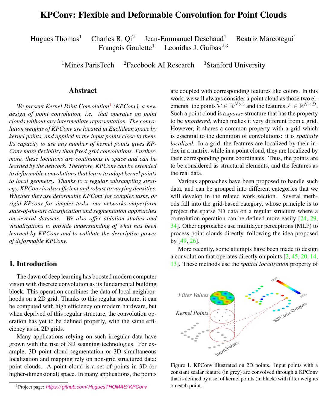
Kernel Point Convolution (KPConv) defines a convolution operation directly on 3D point clouds without intermediate representations (such as voxel grids or tangent planes). Given an input point cloud $\mathcal{P} = \{x_i \in \mathbb{R}^3\}_{i=1}^N$ with associated feature vectors $\mathcal{F} = \{f_i \in \mathbb{R}^{D_{\text{in}}}\}_{i=1}^N$ , the continuous convolution of $\mathcal{F}$ with a spatial kernel $g$ evaluated at a query position $x \in \mathbb{R}^3$ over a spherical neighborhood $\mathcal{N}_x = \{x_i \in \mathcal{P} \mid \|x_i - x\| \le r\}$ of radius $r \in \mathbb{R}_{>0}$ is defined as:

$(\mathcal{F} * g)(x) = \sum_{x_i \in \mathcal{N}_x} g(x_i - x) f_i$

Let $y_i = x_i - x \in \mathcal{B}_r^3 = \{y \in \mathbb{R}^3 \mid \|y\| \le r\}$ . The kernel function $g: \mathcal{B}_r^3 \to \mathbb{R}^{D_{\text{out}} \times D_{\text{in}}}$ is parametrized by $K$ kernel points $\{\tilde{x}_k\}_{k=1}^K \subset \mathcal{B}_r^3$ and corresponding weight matrices $\{W_k\}_{k=1}^K \subset \mathbb{R}^{D_{\text{out}} \times D_{\text{in}}}$ :

$g(y_i) = \sum_{k=1}^K h(y_i, \tilde{x}_k) W_k$

where $h(y_i, \tilde{x}_k)$ is a continuous linear correlation function measuring the spatial proximity between the neighbor offset $y_i$ and the kernel point $\tilde{x}_k$ relative to an influence distance $\sigma \in \mathbb{R}_{>0}$ :

$h(y_i, \tilde{x}_k) = \max\left(0, 1 - \frac{\|y_i - \tilde{x}_k\|}{\sigma}\right)$
Knowl 2 — Deformable Kernel Point Convolution
model/method
Deformable Kernel Point Convolution extends rigid KPConv by learning local 3D shifts that adapt kernel point locations to local geometry at each convolution site $x \in \mathbb{R}^3$ . For $K$ canonical kernel points $\{\tilde{x}_k\}_{k=1}^K \subset \mathcal{B}_r^3$ , the network generates a set of 3D shifts $\Delta(x) = \{\Delta_k(x) \in \mathbb{R}^3\}_{k=1}^K$ :

$(\mathcal{F} * g)(x) = \sum_{x_i \in \mathcal{N}_x} g_{\text{deform}}(x_i - x, \Delta(x)) f_i$

where the deformable kernel function $g_{\text{deform}}$ applies kernel weights at shifted locations:

$g_{\text{deform}}(y_i, \Delta(x)) = \sum_{k=1}^K h(y_i, \tilde{x}_k + \Delta_k(x)) W_k$

Here $y_i = x_i - x$ , $W_k \in \mathbb{R}^{D_{\text{out}} \times D_{\text{in}}}$ denotes the weight matrix for kernel point $k$ , and $h(u, v) = \max\left(0, 1 - \frac{\|u - v\|}{\sigma}\right)$ is the linear correlation function with influence radius $\sigma$ .

The $3K$ offset values forming $\Delta(x)$ are predicted by a rigid KPConv layer operating on the $D_{\text{in}}$ -dimensional input features. During network training, the learning rate for the rigid kernel generating these coordinate shifts is set to $0.1$ times the global network learning rate.
Knowl 3 — Regularization Losses for Deformable KPConv
model/method
In sparse 3D point clouds, unconstrained shift optimization in deformable convolution can cause kernel points to drift into empty regions. When no input points fall within a kernel point's influence radius $\sigma$ , the gradient of the linear correlation function $h$ with respect to that kernel point's shift $\Delta_k(x)$ becomes zero, making the kernel point permanently inactive ("lost"). Additionally, multiple kernel points may collapse onto identical positions.

To enforce geometric adaptation and prevent collapsed or lost kernel points, a regularization loss $\mathcal{L}_{\text{reg}}$ is applied across all convolution query locations $x \in \mathbb{R}^3$ :

$\mathcal{L}_{\text{reg}} = \sum_x \left(\mathcal{L}_{\text{fit}}(x) + \mathcal{L}_{\text{rep}}(x)\right)$

The fitting loss $\mathcal{L}_{\text{fit}}(x)$ penalizes the normalized squared distance between each shifted kernel point and its closest neighbor in $\mathcal{N}_x$ :

$\mathcal{L}_{\text{fit}}(x) = \sum_{k=1}^K \min_{y_i \in \mathcal{N}_x} \left( \frac{\|y_i - (\tilde{x}_k + \Delta_k(x))\|}{\sigma} \right)^2$

The repulsive loss $\mathcal{L}_{\text{rep}}(x)$ penalizes overlapping influence areas between distinct kernel points to prevent collapse:

$\mathcal{L}_{\text{rep}}(x) = \sum_{k=1}^K \sum_{l \neq k} h(\tilde{x}_k + \Delta_k(x), \tilde{x}_l + \Delta_l(x))^2$

During training, $\mathcal{L}_{\text{reg}}$ is added to the primary task loss with a scaling factor of $0.1$ .
Knowl 4 — Kernel Point Position Initialization via Energy Minimization
algorithm
Rigid KPConv requires $K$ kernel points $\{\tilde{x}_k\}_{k=1}^K$ placed regularly inside a sphere $\mathcal{B}_r^3$ . Because regular polyhedral lattices do not exist for arbitrary $K$ , canonical positions are obtained by solving an energy minimization problem that repels points from each other while confining them to the sphere. One kernel point is fixed at the center $(0,0,0)$ , and the remaining $K-1$ points are initialized randomly.

The global energy objective $E_{\text{tot}}$ to be minimized over kernel points $\{\tilde{x}_k\}_{k=1}^K \subset \mathbb{R}^3$ is:

$E_{\text{tot}} = \sum_{k=1}^K \left( E^{\text{att}}(\tilde{x}_k) + \sum_{l \neq k} E^{\text{rep}}_k(\tilde{x}_l) \right)$

where the attractive potential $E^{\text{att}}$ confines points to the origin and the repulsive potential $E^{\text{rep}}_k$ pushes points apart:

$E^{\text{att}}(x) = \|x\|^2, \quad E^{\text{rep}}_k(x) = \frac{1}{\|x - \tilde{x}_k\|}$

Optimization via gradient descent converges to stable regular polyhedral dispositions for specific values of $K$ :
- $K=5$ : Tetrahedron
- $K=7$ : Octahedron (1-4-1 point groups along symmetrical axis)
- $K=13$ : Icosahedron (1-5-5-1 point groups along symmetrical axis)
- $K=15$ : 1-6-6-1 point groups along symmetrical axis
- $K=18$ : 1-5-5-5-1 point groups
- $K=19$ : 1-4-4-4-4-1 point groups
- $K=21$ : 1-6-6-6-1 point groups
- $K=25$ : 4-4-4-4-4-4 point groups
Following optimization, the outer kernel points are rescaled to an average radius of $1.5\sigma$ , providing space coverage with controlled overlap between influence areas.
Knowl 5 — Multi-Scale Grid Subsampling and KPConv Layer Hyperparameters
model/method
To handle non-uniform point densities and build hierarchical architectures, KPConv uses a regular grid subsampling strategy:
1. Grid Subsampling: The input point cloud is partitioned by a 3D grid with cell size $dl_0$ . Support points carrying feature representations at layer $0$ are computed as the spatial barycenters of points within each non-empty grid cell. For classification tasks without input features (e.g. ModelNet40), every point is assigned a constant scalar feature equal to $1$ .
2. Hierarchical Downsampling: At each successive pooling layer $j$ , the grid cell size doubles: $dl_{j+1} = 2 \cdot dlj$ . Downsampled points and their features are generated via "strided KPConv", where neighborhood queries are centered at the subsampled points $N'$ over input points $N$ .
3. Hyperparameter Scaling: At layer $j$ , the kernel point influence distance is set to $\sigma_j = \Sigma \cdot dlj$ . For rigid KPConv, the neighborhood radius is $r_j = 2.5 \sigma_j$ (given the outer kernel points' average radius of $1.5\sigma_j$ ). For deformable KPConv, the neighborhood radius is $r_j = \rho \cdot dlj$ .
The standard hyperparameter values used across experiments are $K = 15$ kernel points, $\Sigma = 1.0$ , and $\rho = 5.0$ .
Knowl 6 — KP-CNN and KP-FCNN Network Architectures
model/method
Two neural network architectures are constructed using KPConv bottleneck blocks analogous to ResNet bottleneck blocks with residual connections, batch normalization, and leaky ReLU activations:
- KP-CNN (Classification): A 5-layer classification network. Each layer contains two convolutional blocks. The first block in layers 2 through 5 uses strided KPConv for spatial pooling. After layer 5, features are aggregated using global average pooling and passed through fully connected layers with dropout ( $0.5$ probability) to a softmax classifier. In deformable KP-CNN models, deformable KPConv blocks are used in the final 5 convolutional blocks (block 2 of layer 3, and both blocks of layers 4 and 5).
- KP-FCNN (Semantic Segmentation): An encoder-decoder fully convolutional network. The encoder is identical to KP-CNN. The decoder uses nearest upsampling to propagate features back to higher point resolutions, concatenates them with intermediate encoder features via skip connections, and processes the combined features using unary convolutions ( $1 \times 1$ convolutions).
- Variable Batching: Point clouds of variable point counts are batched by concatenating coordinates and features along the first tensor dimension up to a target point budget per batch, avoiding zero-padding overhead.

Knowl 7 — 3D Shape Classification and Part Segmentation Performance

data/table

KPConv was evaluated on ModelNet40 (CAD shape classification, 40 classes) using coordinates only (no surface normals, $dl_0 = 2\text{ cm}$ ) and ShapeNetPart (part segmentation, 16 categories, 50 parts). Metrics reported are Overall Accuracy (OA) for ModelNet40, and class-averaged mIoU (mcIoU) and instance-averaged mIoU (mIoU) for ShapeNetPart.

Method	ModelNet40 OA (%)	ShapeNetPart mcIoU (%)	ShapeNetPart mIoU (%)
SPLATNet	-	83.7	85.4
SGPN	-	82.8	85.8
3DmFV-Net	91.6	81.0	84.3
SynSpecCNN	-	82.0	84.7
RSNet	-	81.4	84.9
SpecGCN	91.5	-	85.4
PointNet++	90.7	81.9	85.1
SO-Net	90.9	81.0	84.9
PCNN by Ext	92.3	81.8	85.1
SpiderCNN	90.5	82.4	85.3
MCConv	90.9	-	85.9
FlexConv	90.2	84.7	85.0
PointCNN	92.2	84.6	86.1
DGCNN	92.2	85.0	84.7
SubSparseCNN	-	83.3	86.0
KPConv rigid	92.9	85.0	86.2
KPConv deform	92.7	85.1	86.4

On ModelNet40, rigid KPConv achieves $92.9\%$ OA, slightly higher than deformable KPConv ( $92.7\%$ ), as the simpler classification task does not require additional deformation parameters and is less prone to overfitting with rigid geometric filters. On ShapeNetPart, deformable KPConv achieves the highest scores ( $85.1\%$ mcIoU, $86.4\%$ mIoU), outperforming rigid KPConv and prior point-based architectures.

Knowl 8 — 3D Scene Semantic Segmentation Performance

data/table

KP-FCNN was benchmarked on four indoor and outdoor semantic segmentation datasets: ScanNet (indoor, 20 classes), Semantic3D (reduced-8 outdoor LiDAR challenge, 8 classes), S3DIS (indoor spaces, Area-5 test and 6-fold cross-validation, 13 classes), and Paris-Lille-3D (outdoor mobile LiDAR, 10 classes). Subsampling grid sizes were set to $dl_0 = 4\text{ cm}$ on ScanNet/S3DIS and $dl_0 = 6\text{ cm}$ on Semantic3D/Paris-Lille-3D.

Method	ScanNet mIoU (%)	Semantic3D mIoU (%)	S3DIS Area-5 mIoU (%)	Paris-Lille-3D mIoU (%)
PointNet	-	-	41.1	-
PointNet++	33.9	-	-	-
SnapNet	-	59.1	-	-
SPLATNet	39.3	-	-	-
SegCloud	-	61.3	48.9	-
RF_MSSF	-	62.7	49.8	56.3
Eff3DConv	-	-	51.8	-
TangentConv	43.8	-	52.6	-
MSDVN	-	65.3	54.7	66.9
RSNet	-	-	56.5	-
FCPN	44.7	-	-	-
PointCNN	45.8	-	57.3	-
PCNN	49.8	-	-	-
SPGraph	-	73.2	58.0	-
ParamConv	-	-	58.3	-
SubSparseCNN	72.5	-	-	-
KPConv rigid	68.6	74.6	65.4	72.3
KPConv deform	68.4	73.1	67.1	75.9

On S3DIS $k$ -fold cross-validation, deformable KPConv achieved $70.6\%$ mIoU ( $79.1\%$ mean recall) compared to rigid KPConv at $69.6\%$ mIoU ( $78.1\%$ mean recall). Deformable KPConv outperforms rigid KPConv on datasets with diverse indoor or complex object structures (S3DIS Area-5: $67.1\%$ vs $65.4\%$ ; Paris-Lille-3D: $75.9\%$ vs $72.3\%$ ). Rigid KPConv yields higher scores on datasets dominated by large planar surfaces and lower object variety (Semantic3D: $74.6\%$ vs $73.1\%$ ).

Knowl 9 — Robustness of Deformable KPConv to Kernel Point Reductions
empirical result
An ablation study on the ScanNet validation set evaluated the performance impact of reducing the number of kernel points $K$ from 15 down to 4:
- At $K = 15$ , deformable KPConv achieves approximately $69.2\%$ validation mIoU, whereas rigid KPConv achieves approximately $68.4\%$ validation mIoU.
- When $K$ is reduced to 4 kernel points, deformable KPConv drops by $1.5\%$ mIoU to approximately $67.7\%$ .
- Under the same reduction to $K = 4$ , rigid KPConv drops by $3.5\%$ mIoU to approximately $65.0\%$ .
The smaller performance drop in deformable KPConv indicates that learned coordinate shifts allow a small set of kernel points to adjust their spatial layout dynamically to fit local geometry, providing higher descriptive power per kernel parameter than rigid kernel configurations.
Knowl 10 — Effective Receptive Field Adaptability of Deformable KPConv
empirical result
The Effective Receptive Field (ERF), computed as the gradient magnitude of a network layer's activation at a given point with respect to input point features, exhibits distinct behaviors between rigid and deformable KPConv models (evaluated at layer 4 of KP-FCNN trained on ScanNet):
- Rigid KPConv: Produces an ERF of relatively fixed, isotropic metric radius across all query locations, regardless of whether the query is positioned on large objects, small objects, or planar ground.
- Deformable KPConv: Produces an ERF that dynamically adapts to object size and geometric boundaries. When centered on a large object (such as a bed), the ERF expands to cover the entire structure. When centered on a smaller object (such as a chair), the ERF concentrates within the object boundaries while suppressing influence from adjacent floor points. On large flat surfaces, deformable KPConv reduces activations across uniform planar points and extends toward distant geometric features and structural edges.

Coverage note — Detailed per-class IoU breakdown tables for ShapeNetPart (Table 5) and S3DIS (Tables 6 and 7) were omitted in favor of dataset-level summary tables (Tables 1 and 2), and descriptions of accompanying demonstration videos were omitted as they duplicate paper content.

References

1.Iro Armeni, Ozan Sener, Amir R. Zamir, Helen Jiang, Ioannis Brilakis, Martin Fischer, and Silvio Savarese. 3d semantic parsing of large-scale indoor spaces. In Proceedings of the IEEE Conference on Computer Vision and Pattern Recognition, pages 1534–1543, 2016. http://buildingparser.stanford.edu/dataset.html.
2.Matan Atzmon, Haggai Maron, and Yaron Lipman. Point convolutional neural networks by extension operators. ACM Transactions on Graphics (TOG), 37(4):71, 2018.
3.Yizhak Ben-Shabat, Michael Lindenbaum, and Anath Fischer. 3dmfv: Three-dimensional point cloud classification in real-time using convolutional neural networks. IEEE Robotics and Automation Letters, 3(4):3145–3152, 2018.
4.Alexandre Boulch, Bertrand Le Saux, and Nicolas Audebert. Unstructured point cloud semantic labeling using deep segmentation networks. In Proceedings of the Workshop on 3D Object Retrieval (3DOR), 2017.
5.Michael M. Bronstein, Joan Bruna, Yann LeCun, Arthur Szlam, and Pierre Vandergheynst. Geometric deep learning: going beyond euclidean data. IEEE Signal Processing Magazine, 34(4):18–42, 2017.
6.Angela Dai, Angel X. Chang, Manolis Savva, Maciej Halber, Thomas Funkhouser, and Matthias Nießner. Scannet: Richly-annotated 3d reconstructions of indoor scenes. In Proceedings of the IEEE Conference on Computer Vision and Pattern Recognition, pages 5828–5839, 2017. http://kaldir.vc.in.tum.de/scannet_benchmark.
7.Jifeng Dai, Haozhi Qi, Yuwen Xiong, Yi Li, Guodong Zhang, Han Hu, and Yichen Wei. Deformable convolutional networks. In Proceedings of the IEEE international Conference on Computer Vision, pages 764–773, 2017.
8.Michael Defferrard, Xavier Bresson, and Pierre Vandergheynst. Convolutional neural networks on graphs with fast localized spectral filtering. In Advances in Neural Information Processing Systems, pages 3844–3852, 2016.
9.Benjamin Graham, Martin Engelcke, and Laurens van der Maaten. 3d semantic segmentation with submanifold sparse convolutional networks. In Proceedings of the IEEE Conference on Computer Vision and Pattern Recognition, pages 9224–9232, 2018.
10.Fabian Groh, Patrick Wieschollek, and Hendrik P.A. Lensch. Flex-convolution. In Asian Conference on Computer Vision, pages 105–122. Springer, 2018.
11.Timo Hackel, Nikolay Savinov, Lubor Ladicky, Jan D. Wegner, Konrad Schindler, and Marc Pollefeys. Semantic3d.net: A new large-scale point cloud classification benchmark. arXiv preprint arXiv:1704.03847, 2017. http://www.semantic3d.net.
12.Kaiming He, Xiangyu Zhang, Shaoqing Ren, and Jian Sun. Deep residual learning for image recognition. In Proceedings of the IEEE conference on Computer Vision and Pattern Recognition, pages 770–778, 2016.
13.Pedro Hermosilla, Tobias Ristchel, Pere-Pau Vázquez, Álvaro Vinacua, and Timo Ropinski. Monte carlo convolution for learning on non-uniformly sampled point clouds. ACM Transactions on Graphics (TOG), 37(6):235–1, 2018.
14.Binh-Son Hua, Minh-Khoi Tran, and Sai-Kit Yeung. Pointwise convolutional neural networks. In Proceedings of the IEEE Conference on Computer Vision and Pattern Recognition, pages 984–993, 2018.
15.Qiangui Huang, Weiyue Wang, and Ulrich Neumann. Recurrent slice networks for 3d segmentation of point clouds. In Proceedings of the IEEE Conference on Computer Vision and Pattern Recognition, pages 2626–2635, 2018.
16.Roman Klokov and Victor Lempitsky. Escape from cells: Deep kd-networks for the recognition of 3d point cloud models. In Proceedings of the IEEE International Conference on Computer Vision, pages 863–872, 2017.
17.Loic Landrieu and Martin Simonovsky. Large-scale point cloud semantic segmentation with superpoint graphs. In Proceedings of the IEEE Conference on Computer Vision and Pattern Recognition, pages 4558–4567, 2018.
18.Felix Järemo Lawin, Martin Danelljan, Patrik Tosteberg, Goutam Bhat, Fahad Shahbaz Khan, and Michael Felsberg. Deep projective 3d semantic segmentation. In International Conference on Computer Analysis of Images and Patterns, pages 95–107. Springer, 2017.
19.Jiaxin Li, Ben M. Chen, and Gim Hee Lee. So-net: Self-organizing network for point cloud analysis. In Proceedings of the IEEE Conference on Computer Vision and Pattern Recognition, pages 9397–9406, 2018.
20.Yangyan Li, Rui Bu, Mingchao Sun, Wei Wu, Xinhan Di, and Baoquan Chen. Pointcnn: Convolution on x-transformed points. In Advances in Neural Information Processing Systems, pages 820–830, 2018.
21.Xinhai Liu, Zhizhong Han, Yu-Shen Liu, and Matthias Zwicker. Point2sequence: Learning the shape representation of 3d point clouds with an attention-based sequence to sequence network. arXiv preprint arXiv:1811.02565, 2018.
22.Wenjie Luo, Yujia Li, Raquel Urtasun, and Richard Zemel. Understanding the effective receptive field in deep convolutional neural networks. In Advances in neural information processing systems, pages 4898–4906, 2016.
23.Jonathan Masci, Davide Boscaini, Michael Bronstein, and Pierre Vandergheynst. Geodesic convolutional neural networks on riemannian manifolds. In Proceedings of the IEEE international conference on computer vision workshops, pages 37–45, 2015.
24.Daniel Maturana and Sebastian Scherer. Voxnet: A 3d convolutional neural network for real-time object recognition. In Intelligent Robots and Systems (IROS), 2015 IEEE/RSJ International Conference on, pages 922–928. IEEE, 2015.
25.Federico Monti, Davide Boscaini, Jonathan Masci, Emanuele Rodola, Jan Svoboda, and Michael M. Bronstein. Geometric deep learning on graphs and manifolds using mixture model cnns. In Proceedings of the IEEE Conference on Computer Vision and Pattern Recognition, pages 5115–5124, 2017.
26.Charles R. Qi, Hao Su, Kaichun Mo, and Leonidas J. Guibas. Pointnet: Deep learning on point sets for 3d classification and segmentation. In Proceedings of the IEEE Conference on Computer Vision and Pattern Recognition, pages 652–660, 2017.
27.Charles R. Qi, Li Yi, Hao Su, and Leonidas J. Guibas. Pointnet++: Deep hierarchical feature learning on point sets in a metric space. In Advances in Neural Information Processing Systems, pages 5099–5108, 2017.
28.Dario Rethage, Johanna Wald, Jurgen Sturm, Nassir Navab, and Federico Tombari. Fully-convolutional point networks for large-scale point clouds. In Proceedings of the European Conference on Computer Vision (ECCV), pages 596–611, 2018.
29.Gernot Riegler, Ali Osman Ulusoy, and Andreas Geiger. Octnet: Learning deep 3d representations at high resolutions. In Proceedings of the IEEE Conference on Computer Vision and Pattern Recognition, volume 3, 2017.
30.Xavier Roynard, Jean-Emmanuel Deschaud, and François Goulette. Classification of point cloud scenes with multi-scale voxel deep network. arXiv preprint arXiv:1804.03583, 2018.
31.Xavier Roynard, Jean-Emmanuel Deschaud, and François Goulette. Paris-lille-3d: A large and high-quality ground-truth urban point cloud dataset for automatic segmentation and classification. The International Journal of Robotics Research, 37(6):545–557, 2018. http://npm3d.fr.
32.Yiru Shen, Chen Feng, Yaoqing Yang, and Dong Tian. Mining point cloud local structures by kernel correlation and graph pooling. In Proceedings of the IEEE Conference on Computer Vision and Pattern Recognition, volume 4, 2018.
33.Martin Simonovsky and Nikos Komodakis. Dynamic edge-conditioned filters in convolutional neural networks on graphs. In Proceedings of the IEEE conference on computer vision and pattern recognition, pages 3693–3702, 2017.
34.Hang Su, Varun Jampani, Deqing Sun, Subhransu Maji, Evangelos Kalogerakis, Ming-Hsuan Yang, and Jan Kautz. Splatnet: Sparse lattice networks for point cloud processing. In Proceedings of the IEEE Conference on Computer Vision and Pattern Recognition, pages 2530–2539, 2018.
35.Hang Su, Subhransu Maji, Evangelos Kalogerakis, and Erik Learned-Miller. Multi-view convolutional neural networks for 3d shape recognition. In Proceedings of the IEEE International Conference on Computer Vision, pages 945–953, 2015.
36.Maxim Tatarchenko, Jaesik Park, Vladlen Koltun, and Qian-Yi Zhou. Tangent convolutions for dense prediction in 3d. In Proceedings of the IEEE Conference on Computer Vision and Pattern Recognition, pages 3887–3896, 2018.
37.Lyne Tchapmi, Christopher Choy, Iro Armeni, JunYoung Gwak, and Silvio Savarese. Segcloud: Semantic segmentation of 3d point clouds. In 2017 International Conference on 3D Vision (3DV), pages 537–547. IEEE, 2017.
38.Hugues Thomas, François Goulette, Jean-Emmanuel Deschaud, and Beatriz Marcotegui. Semantic classification of 3d point clouds with multiscale spherical neighborhoods. In 2018 International Conference on 3D Vision (3DV), pages 390–398. IEEE, 2018.
39.Nitika Verma, Edmond Boyer, and Jakob Verbeek. Feastnet: Feature-steered graph convolutions for 3d shape analysis. In Proceedings of the IEEE Conference on Computer Vision and Pattern Recognition, pages 2598–2606, 2018.
40.Chu Wang, Babak Samari, and Kaleem Siddiqi. Local spectral graph convolution for point set feature learning. In Proceedings of the European Conference on Computer Vision (ECCV), pages 52–66, 2018.
41.Shenlong Wang, Simon Suo, Wei-Chiu Ma, Andrei Pokrovsky, and Raquel Urtasun. Deep parametric continuous convolutional neural networks. In Proceedings of the IEEE Conference on Computer Vision and Pattern Recognition, pages 2589–2597, 2018.
42.Weiyue Wang, Ronald Yu, Qiangui Huang, and Ulrich Neumann. Sgpn: Similarity group proposal network for 3d point cloud instance segmentation. In Proceedings of the IEEE Conference on Computer Vision and Pattern Recognition, pages 2569–2578, 2018.
43.Yue Wang, Yongbin Sun, Ziwei Liu, Sanjay E. Sarma, Michael M. Bronstein, and Justin M. Solomon. Dynamic graph cnn for learning on point clouds. ACM Transactions on Graphics (TOG), 2019.
44.Zhirong Wu, Shuran Song, Aditya Khosla, Fisher Yu, Linguang Zhang, Xiaoou Tang, and Jianxiong Xiao. 3d shapenets: A deep representation for volumetric shapes. In Proceedings of the IEEE conference on Computer Vision and Pattern Recognition, pages 1912–1920, 2015.
45.Yifan Xu, Tianqi Fan, Mingye Xu, Long Zeng, and Yu Qiao. Spidercnn: Deep learning on point sets with parameterized convolutional filters. In Proceedings of the European Conference on Computer Vision (ECCV), pages 87–102, 2018.
46.Xiaoqing Ye, Jiamao Li, Hexiao Huang, Liang Du, and Xiaolin Zhang. 3d recurrent neural networks with context fusion for point cloud semantic segmentation. In Proceedings of the European Conference on Computer Vision (ECCV), pages 415–430. Springer, 2018.
47.Li Yi, Vladimir G. Kim, Duygu Ceylan, I Shen, Mengyan Yan, Hao Su, Cewu Lu, Qixing Huang, Alla Sheffer, Leonidas J. Guibas, et al. A scalable active framework for region annotation in 3d shape collections. ACM Transactions on Graphics (TOG), 35(6):210, 2016.
48.Li Yi, Hao Su, Xingwen Guo, and Leonidas J. Guibas. Syncspeccnn: Synchronized spectral cnn for 3d shape segmentation. In CVPR, pages 6584–6592, 2017.
49.Manzil Zaheer, Satwik Kottur, Siamak Ravanbakhsh, Barnabas Poczos, Ruslan R. Salakhutdinov, and Alexander J Smola. Deep sets. In Advances in Neural Information Processing Systems, pages 3391–3401, 2017.
50.Chris Zhang, Wenjie Luo, and Raquel Urtasun. Efficient convolutions for real-time semantic segmentation of 3d point clouds. In 2018 International Conference on 3D Vision (3DV), pages 399–408. IEEE, 2018.

Citation

MLA

Thomas, H., et al. “KPConv: Flexible and Deformable Convolution for Point Clouds”. arXiv, 2019, http://arxiv.org/abs/1904.08889v2.

APA

Thomas, H., Qi, C. R., Deschaud, J.-E., Marcotegui, B., Goulette, F., & Guibas, L. J. (2019). KPConv: Flexible and Deformable Convolution for Point Clouds. arXiv. http://arxiv.org/abs/1904.08889v2

Chicago

Thomas, H., C. R. Qi, J.-E. Deschaud, B. Marcotegui, F. Goulette, and L. J. Guibas. 2019. “KPConv: Flexible and Deformable Convolution for Point Clouds”. arXiv. http://arxiv.org/abs/1904.08889v2.

Harvard

Thomas, H. et al. (2019) “KPConv: Flexible and Deformable Convolution for Point Clouds”, arXiv [Preprint]. Available at: http://arxiv.org/abs/1904.08889v2.

Vancouver

1. Thomas H, Qi CR, Deschaud J-E, Marcotegui B, Goulette F, Guibas LJ (2019) KPConv: Flexible and Deformable Convolution for Point Clouds. arXiv

BibTeX

@article{thomas2019kpconv,
  title = {KPConv: Flexible and Deformable Convolution for Point Clouds},
  author = {Thomas, Hugues and Qi, Charles R. and Deschaud, Jean-Emmanuel and Marcotegui, Beatriz and Goulette, François and Guibas, Leonidas J.},
  year = {2019},
  journal = {arXiv},
  url = {http://arxiv.org/abs/1904.08889v2},
  eprint = {1904.08889}
}

Metadata:arXiv

Source Code

This paper has an official code repository available. Click below to access the source code.

View Repository

Access the Paper

This paper is available from its original source. Click below to access the PDF.

Open PDF

License: IEEE

KPConv: Flexible and Deformable Convolution for Point Clouds

Abstract

Topics

Keywords

Table of Contents

Knowls

Knowl 1 — Kernel Point Convolution (KPConv) Operator

Knowl 2 — Deformable Kernel Point Convolution

Knowl 3 — Regularization Losses for Deformable KPConv

Knowl 4 — Kernel Point Position Initialization via Energy Minimization

Knowl 5 — Multi-Scale Grid Subsampling and KPConv Layer Hyperparameters

Knowl 6 — KP-CNN and KP-FCNN Network Architectures