Cyclical Learning Rates for Training Neural Networks

Leslie N. Smith

article2017WACV3,011 citations

Introduces cyclical learning rates and a simple boundary-estimation test to eliminate tedious hyperparameter tuning, allowing deep neural networks to train in fewer iterations and reach higher classification accuracy.

Listen

The paper addresses a longstanding challenge in training deep neural networks: selecting and scheduling the global learning rate, widely regarded as the single most important hyper-parameter. Poor choices cause slow convergence or outright divergence, while conventional practice of running many fixed-rate or monotonically decreasing trials consumes substantial time and compute. The work evaluates whether a simple cyclical schedule that varies the learning rate between two bounds can match or exceed the accuracy of carefully tuned fixed schedules, often in fewer iterations and with far less experimentation.

The central objective is to show that allowing the learning rate to rise and fall repeatedly between empirically determined minimum and maximum values produces near-optimal classification performance across standard architectures and datasets while largely eliminating manual tuning. The approach relies on a shortlearning-rate range testin which the rate is increased linearly over a few epochs; the resulting accuracy curve directly supplies the two bounds. These bounds are then used in one of several cyclical policies (triangular, triangular2, or exponential-range) whose cycle length is set to a small multiple of the number of iterations per epoch. Experiments cover CIFAR-10 and CIFAR-100 with Caffe’s baseline network, ResNets, Stochastic Depth networks, and DenseNets, plus ImageNet with AlexNet and GoogLeNet.

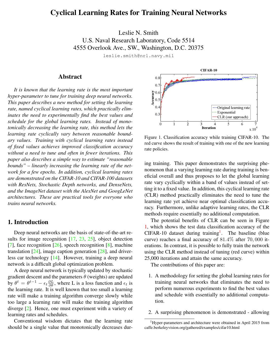
The most important results are that the triangular2 policy reaches the baseline accuracy of 81.4 percent on CIFAR-10 after only 25 000 iterations instead of 70 000, that the same policy improves GoogLeNet validation accuracy by 1.4 percentage points over a reasonable fixed schedule, and that the exponential-range policy yields both higher final accuracy and earlier stopping on both CIFAR-10 and ImageNet. Across all tested residual-style networks the cyclical schedules match or exceed fixed-rate performance even when the fixed rate is already near-optimal, and the gains persist when cyclical schedules are combined with adaptive methods such as Nesterov or Adam. A secondary but practical finding is that accuracy reliably peaks at the end of each cycle, providing a clear signal for when to reduce the rate or halt training.

These outcomes imply that practitioners can obtain competitive or superior models with substantially less hyper-parameter search and with little or no added computation, lowering both training cost and the risk of suboptimal convergence. The method is especially attractive when a new architecture or dataset is first encountered, because a single short range test replaces dozens of full training runs.

The paper recommends running the range test once, selecting bounds from the resulting curve, and then training with a cyclical policy for three to five cycles before dropping the rate or stopping; the same workflow applies whether or not adaptive per-parameter methods are also used. Further work is needed to confirm equivalent behavior on recurrent networks and to develop supporting theory.

The findings rest on well-known public datasets and reproducible code releases, yet remain bounded by the architectures and image-classification tasks examined; results on other domains or loss landscapes could differ. Overall is high for the reported settings because multiple independent implementations and repeated runs produce consistent gains.

  • Paper: Decoupled Weight Decay Regularization, Ilya Loshchilov et al. (2019). The source's exploration of learning rate schedules naturally extends into decoupled weight decay techniques like AdamW, which are critical for optimal performance with advanced schedules.
  • Paper: Accurate, Large Minibatch SGD: Training ImageNet in 1 Hour, Priya Goyal et al. (2017). Large-minibatch training builds upon adaptive learning rate insights to scale optimization successfully across distributed hardware.
Cover for Cyclical Learning Rates for Training Neural Networks

Abstract

It is known that the learning rate is the most important hyper-parameter to tune for training deep neural networks. This paper describes a new method for setting the learning rate, named cyclical learning rates, which practically eliminates the need to experimentally find the best values and schedule for the global learning rates. Instead of monotonically decreasing the learning rate, this method lets the learning rate cyclically vary between reasonable boundary values. Training with cyclical learning rates instead of fixed values achieves improved classification accuracy without a need to tune and often in fewer iterations. This paper also describes a simple way to estimate "reasonable bounds" -- linearly increasing the learning rate of the network for a few epochs. In addition, cyclical learning rates are demonstrated on the CIFAR-10 and CIFAR-100 datasets with ResNets, Stochastic Depth networks, and DenseNets, and the ImageNet dataset with the AlexNet and GoogLeNet architectures. These are practical tools for everyone who trains neural networks.

Table of Contents

  • 1 Introduction
  • 2 Related work
  • 3 Optimal Learning Rates
  • 3.1 Cyclical Learning Rates
  • 3.2 How can one estimate a good value for the cycle length?
  • 3.3 How can one estimate reasonable minimum and maximum boundary values?
  • 4 Experiments
  • 4.1 CIFAR-10 and CIFAR-100
  • 4.1.1 Caffe’s CIFAR-10 architecture
  • 4.1.2 ResNets, Stochastic Depth, and DenseNets
  • 4.2 ImageNet
  • 4.2.1 AlexNet
  • 4.2.2 GoogLeNet/Inception Architecture
  • 5 Conclusions
  • References
  • A Instructions for adding CLR to Caffe
  • B Instructions for adding CLR to Keras

Knowls

  1. Knowl 1 — Triangular Cyclical Learning Rate Schedule

    model/method

    The triangular cyclical learning rate (CLR) policy varies the global learning rate ηt\eta_t linearly between a lower bound ηmin\eta_{\min} (base learning rate) and an upper bound ηmax\eta_{\max} (maximum learning rate) over a defined cycle length.

    Let t0t \ge 0 denote the current training iteration, and let LstepL_{\text{step}} (stepsize) denote the number of iterations in half a cycle (one linear ramp up or ramp down). A full cycle has duration 2Lstep2 L_{\text{step}}. The cycle index and relative position within the cycle are defined as:

    cycle=1+t2Lstep\text{cycle} = \left\lfloor 1 + \frac{t}{2 L_{\text{step}}} \right\rfloor

    x=tLstep2cycle+1x = \left| \frac{t}{L_{\text{step}}} - 2 \cdot \text{cycle} + 1 \right|

    The learning rate ηt\eta_t at iteration tt is computed as:

    ηt=ηmin+(ηmaxηmin)max(0,1x)\eta_t = \eta_{\min} + (\eta_{\max} - \eta_{\min}) \cdot \max(0, 1 - x)

    Under this policy, ηt\eta_t increases linearly from ηmin\eta_{\min} to ηmax\eta_{\max} during the first half of the cycle (LstepL_{\text{step}} iterations) and decreases linearly back to ηmin\eta_{\min} during the second half. Functional forms including Welch (parabolic) and Hann (sinusoidal) windows yield equivalent empirical performance, making the linear triangular schedule preferred due to its simplicity.

  2. Knowl 2 — Cyclical Learning Rate Policy Variants: triangular2 and exp_range

    model/method

    Two variations of the triangular cyclical learning rate policy modify how boundary amplitudes scale throughout training:

    1. triangular2 Policy: Retains the linear triangular shape, but the amplitude difference (ηmaxηmin)(\eta_{\max} - \eta_{\min}) is halved at the end of each full cycle. For cycle index c=1+t2Lstepc = \lfloor 1 + \frac{t}{2 L_{\text{step}}} \rfloor and x=tLstep2c+1x = | \frac{t}{L_{\text{step}}} - 2 c + 1 |, the learning rate is:

    ηt=ηmin+ηmaxηmin2c1max(0,1x)\eta_t = \eta_{\min} + \frac{\eta_{\max} - \eta_{\min}}{2^{c - 1}} \cdot \max(0, 1 - x)

    1. exp_range Policy: Modulates both boundary boundaries by an exponential decay factor γt\gamma^t at each iteration tt, where γ(0,1)\gamma \in (0, 1) is a decay constant (e.g., γ=0.99994\gamma = 0.99994 or γ=0.99998\gamma = 0.99998):

    ηt=ηminγt+(ηmaxηmin)γtmax(0,1x)\eta_t = \eta_{\min} \gamma^t + (\eta_{\max} - \eta_{\min}) \gamma^t \cdot \max(0, 1 - x)

  3. Knowl 3 — Learning Rate Range Test

    algorithm

    The Learning Rate Range Test (LR range test) is an empirical diagnostic procedure to determine suitable lower (etamin\\eta_{\\min}) and upper (etamax\\eta_{\\max}) learning rate boundaries for training a neural network on a new dataset or architecture.

    Input: Neural network model M\mathcal{M}, training dataset D\mathcal{D}, starting learning rate ηstart\eta_{\text{start}}, terminating learning rate ηend\eta_{\text{end}}, total test iterations NN (spanning 1 to 8 epochs)
    Output: Minimum learning rate boundary ηmin\eta_{\min}, maximum learning rate boundary ηmax\eta_{\max}
    Initialize model M\mathcal{M} with initial weights
    for iteration t=1t = 1 to NN do
        ηtηstart+(tN)(ηendηstart)\eta_t \leftarrow \eta_{\text{start}} + \left(\frac{t}{N}\right) (\eta_{\text{end}} - \eta_{\text{start}})
        Sample mini-batch BtDB_t \sim \mathcal{D}
        Update parameters of M\mathcal{M} via stochastic gradient descent with learning rate ηt\eta_t on BtB_t
        Evaluate and record validation/training accuracy AtA_t (or loss LtL_t)
    end for
    Plot accuracy AtA_t against learning rate ηt\eta_t
    ηmin\eta_{\min} \leftarrow learning rate value where accuracy first begins to increase
    ηmax\eta_{\max} \leftarrow learning rate value where accuracy peaks, becomes ragged, or begins to drop
    Optional: if only ηmax\eta_{\max} is identified, set ηmin13ηmax\eta_{\min} \leftarrow \frac{1}{3} \eta_{\max} or 14ηmax\frac{1}{4} \eta_{\max}
    return ηmin,ηmax\eta_{\min}, \eta_{\max}

    The identified boundaries [ηmin,ηmax][ \eta_{\min}, \eta_{\max}] form the operational range for cyclical learning rate schedules.

  4. Knowl 4 — Cycle Length and Training Termination Heuristics

    model/method

    Setting the cycle length and stopping criteria for cyclical learning rates follows specific operational rules:

    • Stepsize Calculation: The stepsize parameter LstepL_{\text{step}} represents the half-cycle duration in iterations. Given an epoch length Nepoch=Ntrain/BN_{\text{epoch}} = N_{\text{train}} / B (where NtrainN_{\text{train}} is the number of training samples and BB is the batch size), setting Lstep[2Nepoch,10Nepoch]L_{\text{step}} \in [2 \cdot N_{\text{epoch}}, 10 \cdot N_{\text{epoch}}] produces robust optimization performance.
    • Cycle Count: Replacing each step of a standard fixed learning rate schedule with at least 3 full cycles trains network weights near convergence; running 4 or more cycles achieves higher final accuracy.
    • Stopping Condition: Training runs should be terminated at the conclusion of a full cycle when ηt=ηmin\eta_t = \eta_{\min}, which corresponds to the point where validation classification accuracy peaks.
  5. Knowl 5 — Saddle Point Plateau Traversal Mechanism in Loss Landscapes

    theoretical result

    The theoretical justification for why cyclical learning rates improve optimization performance centers on non-convex loss function topology:

    1. In deep neural network loss surfaces, optimization difficulty predominantly arises from saddle points rather than poor local minima.
    2. Saddle points feature flat plateaus with small gradients, which cause gradient descent with small fixed learning rates to stall.
    3. Periodically increasing the learning rate provides larger parameter update steps, enabling the optimizer to rapidly traverse flat saddle point plateaus despite temporary increases in loss or drops in accuracy.
    4. Subsequent reduction of the learning rate allows the optimizer to settle into and fine-tune parameters within nearby local minima.
    5. Cycling continuously within [ηmin,ηmax][ \eta_{\min}, \eta_{\max}] ensures that near-optimal learning rates are sampled throughout training without requiring precise hyperparameter schedules.
  6. Knowl 6 — Bidirectional Cycle Requirement for Cyclical Learning Rate Benefits

    empirical result

    To evaluate whether the benefits of cyclical learning rates stem solely from decreasing the learning rate, an experimental decay policy was tested against the triangular policy on CIFAR-10. The decay policy started at ηmax=0.007\eta_{\max} = 0.007, linearly decreased to ηmin=0.001\eta_{\min} = 0.001 over Lstep=4000L_{\text{step}} = 4000 iterations, and remained fixed at 0.0010.001 thereafter.

    • Linear decay policy: Achieved 78.5%78.5\% final test accuracy at 25,000 iterations.
    • Standard fixed learning rate baseline (0.0010.001): Achieved 81.4%81.4\% final test accuracy at 70,000 iterations.
    • triangular2 policy: Achieved 81.4%81.4\% final test accuracy at 25,000 iterations (2.8×2.8\times faster convergence).
    • exp_range policy: Achieved 82.2%82.2\% final test accuracy at 42,000 iterations.

    The substantially lower accuracy of the unidirectional decay policy (78.5%78.5\%) confirms that both periodic increases and decreases in the learning rate are necessary to achieve the convergence and generalization gains of CLR.

  7. Knowl 7 — Classification Accuracy and Speedup Across Schedules on CIFAR-10 and ImageNet

    data/table

    The table compares final test classification accuracies and iteration counts across fixed, exponential decay, and cyclical learning rate policies on CIFAR-10, AlexNet (ImageNet), and GoogLeNet (ImageNet):

    Dataset / Model LR Policy Iterations Accuracy (%)
    CIFAR-10 fixed 70,000 81.4
    CIFAR-10 triangular2 25,000 81.4
    CIFAR-10 decay 25,000 78.5
    CIFAR-10 exp 70,000 79.1
    CIFAR-10 exp_range 42,000 82.2
    AlexNet (ImageNet) fixed 400,000 58.0
    AlexNet (ImageNet) triangular2 400,000 58.4
    AlexNet (ImageNet) exp 300,000 56.0
    AlexNet (ImageNet) exp 460,000 56.5
    AlexNet (ImageNet) exp_range 300,000 56.5
    GoogLeNet (ImageNet) fixed 420,000 63.0
    GoogLeNet (ImageNet) triangular2 420,000 64.4
    GoogLeNet (ImageNet) exp 240,000 58.2
    GoogLeNet (ImageNet) exp_range 240,000 60.2

    Key observations:

    • On CIFAR-10, triangular2 reaches the baseline accuracy (81.4%81.4\%) in 25,000 iterations versus 70,000 iterations for the fixed policy. exp_range improves accuracy to 82.2%82.2\% within 42,000 iterations.
    • On AlexNet, exp_range achieves 56.5%56.5\% accuracy in 300,000 iterations, whereas standard exponential decay requires 460,000 iterations (35%35\% fewer iterations).
    • On GoogLeNet, triangular2 outperforms the fixed baseline by 1.4%1.4\% (64.4%64.4\% vs 63.0%63.0\%), and exp_range outperforms exponential decay by 2.0%2.0\% (60.2%60.2\% vs 58.2%58.2\%).
  8. Knowl 8 — CLR Performance on Sigmoid Activations with Batch Normalization

    empirical result

    On a CIFAR-10 convolutional network architecture configured with sigmoid non-linearities and batch normalization:

    • Training with a fixed learning rate yields a final classification accuracy of 60.8%60.8\%.
    • Training with a cyclical learning rate yields a final classification accuracy of 72.2%72.2\%.

    This represents an absolute accuracy improvement of 11.4%11.4\%, demonstrating that cyclical learning rates substantially aid optimization in networks combining saturating activation functions with batch normalization.

  9. Knowl 9 — Integration of Cyclical Learning Rates with Adaptive Optimization Algorithms

    data/table

    Cyclical learning rates can be combined with adaptive learning rate optimizers by cyclically varying their global base learning rate parameter between bounds determined via the LR range test. The table reports final test accuracies on CIFAR-10:

    Optimizer Bounds (ηminηmax\eta_{\min} - \eta_{\max}) LR Policy Iterations Accuracy (%)
    Nesterov 0.001 – 0.006 fixed 70,000 82.1
    Nesterov 0.001 – 0.006 triangular 25,000 81.3
    Adam 0.0005 – 0.002 fixed 70,000 81.4
    Adam 0.0005 – 0.002 triangular 25,000 79.8
    Adam 0.0005 – 0.002 triangular 70,000 81.1
    RMSprop 0.0001 – 0.0003 fixed 70,000 75.2
    RMSprop 0.0001 – 0.0003 triangular 25,000 72.8
    RMSprop 0.0001 – 0.0003 triangular 70,000 75.1
    AdaGrad 0.003 – 0.035 fixed 70,000 74.6
    AdaGrad 0.003 – 0.035 triangular 25,000 76.0
    AdaDelta 0.01 – 0.1 fixed 70,000 67.3
    AdaDelta 0.01 – 0.1 triangular 25,000 67.3

    Results demonstrate that CLR provides computational speedups when combined with adaptive methods: Nesterov + CLR achieves near-baseline accuracy (81.3%81.3\%) in 25,000 iterations (2.8×2.8\times speedup), AdaDelta + CLR reaches 67.3%67.3\% in 25,000 iterations matching 70,000 fixed iterations, and AdaGrad + CLR achieves 76.0%76.0\% in 25,000 iterations, exceeding 70,000 fixed iterations (74.6%74.6\%).

  10. Knowl 10 — Empirical Evaluation of CLR on Deep Residual and Dense Architectures

    data/table

    The table reports average final classification accuracy across 5 runs on CIFAR-10 and CIFAR-100 for ResNets, Stochastic Depth (SD) networks, and DenseNets comparing fixed baseline learning rates (0.1, 0.2, 0.3) against cyclical learning rates:

    Architecture CIFAR-10 Accuracy (%) CIFAR-100 Accuracy (%)
    ResNet (fixed η=0.1\eta = 0.1) 92.8 71.2
    ResNet (fixed η=0.2\eta = 0.2) 93.3 71.6
    ResNet (fixed η=0.3\eta = 0.3) 91.8 71.9
    ResNet + CLR (η[0.1,0.3]\eta \in [0.1, 0.3]) 93.6 72.5
    Stochastic Depth (fixed η=0.1\eta = 0.1) 94.6 75.2
    Stochastic Depth (fixed η=0.2\eta = 0.2) 94.5 75.2
    Stochastic Depth (fixed η=0.3\eta = 0.3) 94.2 74.6
    Stochastic Depth + CLR (η[0.1,0.3]\eta \in [0.1, 0.3]) 94.5 75.4
    DenseNet (fixed η=0.1\eta = 0.1) 94.5 75.2
    DenseNet (fixed η=0.2\eta = 0.2) 94.5 75.3
    DenseNet (fixed η=0.3\eta = 0.3) 94.2 74.5
    DenseNet + CLR (η[0.1,0.2]\eta \in [0.1, 0.2]) 94.9 75.9

    Applying CLR with bounds determined via the LR range test matches or exceeds the best fixed learning rate across all three residual families on both datasets, reaching 93.6%93.6\% on ResNet (CIFAR-10), 75.4%75.4\% on Stochastic Depth (CIFAR-100), and 94.9%94.9\% / 75.9%75.9\% on DenseNet.

Coverage note — No substantial contributed material was omitted; framework-specific code snippets for Caffe and Torch are represented by their mathematical definitions and algorithmic specifications.

References

  1. 1.K. Bache, D. DeCoste, and P. Smyth. Hot swapping for online adaptation of optimization hyperparameters. arXiv preprint arXiv:1412.6599, 2014. 2
  2. 2.Y. Bengio. Neural Networks: Tricks of the Trade, chapter Practical recommendations for gradient-based training of deep architectures, pages 437–478. Springer Berlin Heidelberg, 2012. 1, 2, 4
  3. 3.T. M. Breuel. The effects of hyperparameters on sgd training of neural networks. arXiv preprint arXiv:1508.02788, 2015. 2
  4. 4.Y. N. Dauphin, H. de Vries, J. Chung, and Y. Bengio. Rmsprop and equilibrated adaptive learning rates for non-convex optimization. arXiv preprint arXiv:1502.04390, 2015. 2
  5. 5.J. Duchi, E. Hazan, and Y. Singer. Adaptive subgradient methods for online learning and stochastic optimization. The Journal of Machine Learning Research, 12:2121–2159, 2011. 2, 5
  6. 6.A. P. George and W. B. Powell. Adaptive stepsizes for recursive estimation with applications in approximate dynamic programming. Machine learning, 65(1):167–198, 2006. 2
  7. 7.R. Girshick, J. Donahue, T. Darrell, and J. Malik. Rich feature hierarchies for accurate object detection and semantic segmentation. In Computer Vision and Pattern Recognition (CVPR), 2014 IEEE Conference on, pages 580–587. IEEE, 2014. 1
  8. 8.A. Graves and N. Jaitly. Towards end-to-end speech recognition with recurrent neural networks. In Proceedings of the 31st International Conference on Machine Learning (ICML-14), pages 1764–1772, 2014. 1
  9. 9.C. Gulcehre and Y. Bengio. Adasecant: Robust adaptive secant method for stochastic gradient. arXiv preprint arXiv:1412.7419, 2014. 2
  10. 10.K. He, X. Zhang, S. Ren, and J. Sun. Deep residual learning for image recognition. Computer Vision and Pattern Recognition (CVPR), 2016 IEEE Conference on, 2015. 5, 6
  11. 11.K. He, X. Zhang, S. Ren, and J. Sun. Identity mappings in deep residual networks. arXiv preprint arXiv:1603.05027, 2016. 5, 6
  12. 12.G. Huang, Z. Liu, and K. Q. Weinberger. Densely connected convolutional networks. arXiv preprint arXiv:1608.06993, 2016. 5, 6
  13. 13.G. Huang, Y. Sun, Z. Liu, D. Sedra, and K. Weinberger. Deep networks with stochastic depth. arXiv preprint arXiv:1603.09382, 2016. 5, 6
  14. 14.B. Huval, T. Wang, S. Tandon, J. Kiske, W. Song, J. Pazhayampallil, M. Andriluka, R. Cheng-Yue, F. Mujica, A. Coates, et al. An empirical evaluation of deep learning on highway driving. arXiv preprint arXiv:1504.01716, 2015. 1
  15. 15.S. Ioffe and C. Szegedy. Batch normalization: Accelerating deep network training by reducing internal covariate shift. arXiv preprint arXiv:1502.03167, 2015. 5
  16. 16.D. Kingma and J. Lei-Ba. Adam: a method for stochastic optimization. arXiv preprint arXiv:1412.6980, 2015. 2, 5
  17. 17.A. Krizhevsky, I. Sutskever, and G. E. Hinton. Imagenet classification with deep convolutional neural networks. Advances in neural information processing systems, 2012. 1, 2, 6
  18. 18.I. Loshchilov and F. Hutter. Sgdr: Stochastic gradient descent with restarts. arXiv preprint arXiv:1608.03983, 2016. 2
  19. 19.Y. Nesterov. A method of solving a convex programming problem with convergence rate o (1/k2). In Soviet Mathematics Doklady, volume 27, pages 372–376, 1983. 5
  20. 20.S. Ruder. An overview of gradient descent optimization algorithms. arXiv preprint arXiv:1600.04747, 2016. 2
  21. 21.O. Russakovsky, J. Deng, H. Su, J. Krause, S. Satheesh, S. Ma, Z. Huang, A. Karpathy, A. Khosla, M. Bernstein, A. C. Berg, and L. Fei-Fei. ImageNet Large Scale Visual Recognition Challenge. International Journal of Computer Vision (IJCV), 2015. 6
  22. 22.T. Schaul, S. Zhang, and Y. LeCun. No more pesky learning rates. arXiv preprint arXiv:1206.1106, 2012. 2
  23. 23.K. Simonyan and A. Zisserman. Very deep convolutional networks for large-scale image recognition. arXiv preprint arXiv:1409.1556, 2014. 1
  24. 24.I. Sutskever, O. Vinyals, and Q. V. Le. Sequence to sequence learning with neural networks. In Advances in Neural Information Processing Systems, pages 3104–3112, 2014. 1
  25. 25.C. Szegedy, W. Liu, Y. Jia, P. Sermanet, S. Reed, D. Anguelov, D. Erhan, V. Vanhoucke, and A. Rabinovich. Going deeper with convolutions. arXiv preprint arXiv:1409.4842, 2014. 1, 2, 7
  26. 26.Y. Taigman, M. Yang, M. Ranzato, and L. Wolf. Deepface: Closing the gap to human-level performance in face verification. In Computer Vision and Pattern Recognition (CVPR), 2014 IEEE Conference on, pages 1701–1708. IEEE, 2014. 1
  27. 27.T. Tieleman and G. Hinton. Lecture 6.5-rmsprop: Divide the gradient by a running average of its recent magnitude. COURSERA: Neural Networks for Machine Learning, 4, 2012. 2, 5
  28. 28.O. Vinyals, A. Toshev, S. Bengio, and D. Erhan. Show and tell: A neural image caption generator. arXiv preprint arXiv:1411.4555, 2014. 1
  29. 29.M. D. Zeiler. Adadelta: an adaptive learning rate method. arXiv preprint arXiv:1212.5701, 2012. 2, 5

Citation

MLA
Smith, L. N. “Cyclical Learning Rates for Training Neural Networks”. 2017 IEEE Winter Conference on Applications of Computer Vision (WACV), 2017, pp. 464–72, https://doi.org/10.1109/WACV.2017.58.
APA
Smith, L. N. (2017). Cyclical Learning Rates for Training Neural Networks. 2017 IEEE Winter Conference on Applications of Computer Vision (WACV), 464–472. https://doi.org/10.1109/WACV.2017.58
Chicago
Smith, L. N. 2017. “Cyclical Learning Rates for Training Neural Networks”. 2017 IEEE Winter Conference on Applications of Computer Vision (WACV), 464–72. https://doi.org/10.1109/WACV.2017.58.
Harvard
Smith, L.N. (2017) “Cyclical Learning Rates for Training Neural Networks”, 2017 IEEE Winter Conference on Applications of Computer Vision (WACV). IEEE, pp. 464–472. Available at: https://doi.org/10.1109/WACV.2017.58.
Vancouver
1. Smith LN (2017) Cyclical Learning Rates for Training Neural Networks. In: 2017 IEEE Winter Conference on Applications of Computer Vision (WACV). IEEE, pp 464–472

BibTeX

@inproceedings{Smith_2017, title={Cyclical Learning Rates for Training Neural Networks}, url={http://dx.doi.org/10.1109/WACV.2017.58}, DOI={10.1109/wacv.2017.58}, booktitle={2017 IEEE Winter Conference on Applications of Computer Vision (WACV)}, publisher={IEEE}, author={Smith, Leslie N.}, year={2017}, month=Mar, pages={464–472} }
Metadata:Crossref

Access the Paper

This paper is available from its original source. Click below to access the PDF.

Open PDF

License: IEEE