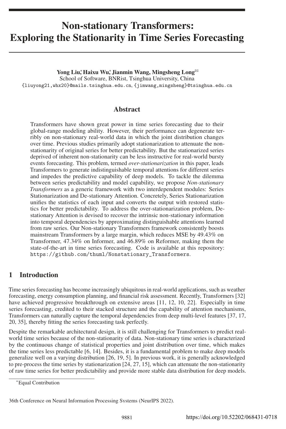
Non-stationary Transformers: Exploring the Stationarity in Time Series Forecasting

Yong LiuHaixu WuJianmin WangMingsheng Long

article2022NeurIPS781 citations

Develops the Non-stationary Transformer framework to solve over-stationarization in time series forecasting by recovering intrinsic temporal dependencies within attention mechanisms, reducing forecasting error by nearly half across standard architectures.

Listen

Real-world time series forecasting is critical for operational planning, energy management, weather tracking, and financial risk assessment. In practical deployments, however, incoming data streams regularly exhibit non-stationarity—meaning their statistical properties, such as mean and standard deviation, continually shift over time. Standard machine learning solutions routinely pre-process data through stationarization techniques to smooth out these fluctuations and improve predictability. However, removing intrinsic variations causes a serious side effect called over-stationarization: attention-based models lose the ability to distinguish eventful, bursty temporal patterns from routine data, causing deep models to produce overly flat and generic forecasts.

The article introduces and evaluates Non-stationary Transformers, a generic framework designed to eliminate this trade-off. The objective is to boost time series predictability through input-output normalization while simultaneously re-integrating essential non-stationary dynamics directly into the model's internal attention mechanism.

The researchers assessed this approach by wrapping standard Transformer architectures and their efficient variants with two complementary components: Series Stationarization and De-stationary Attention. Series Stationarization normalizes incoming data chunks and restores original statistics at the output without adding learnable parameters. De-stationary Attention applies a lightweight multilayer perceptron projector to learn non-stationary scaling and shifting factors from raw statistics, using them to rescale attention calculations. The approach was tested across six benchmark datasets spanning electricity consumption, traffic patterns, influenza illness rates, currency exchange rates, and meteorological records across varied forecast lengths.

The evaluation produced four primary findings. First, integrating the framework consistently elevated performance across all tested benchmarks, achieving state-of-the-art accuracy in both multivariate and univariate forecasting. Second, the framework delivered substantial error reductions on standard Transformer variants, decreasing mean squared error by 49.43% on vanilla Transformer, 47.34% on Informer, 46.89% on Reformer, and 10.57% on Autoformer. Third, accuracy gains were most pronounced on datasets exhibiting the greatest statistical volatility; for instance, the model reduced mean squared error by 17% on exchange rates and 25% on influenza rate forecasts over long prediction horizons compared to prior state-of-the-art methods. Fourth, statistical validation confirmed that predictions generated with De-stationary Attention closely matched ground-truth stationarity levels within a 97% to 103% margin, preventing the over-smoothing observed in traditional stationarization methods.

These findings demonstrate that organizations do not need to choose between data stability and responsiveness to real-world fluctuations. Prior stationarization approaches degraded the expressive power of Transformer attention mechanisms by treating all normalized series identically. By reintroducing raw statistical factors inside the attention layer, deep forecasting models capture sudden shifts and extreme events effectively without compromising baseline stability, offering improved forecast reliability for high-stakes operational planning.

Organizations deploying Transformer architectures for time series forecasting should adopt this framework as an efficient, plug-and-play upgrade. Because the modifications introduce minimal computational overhead and preserve native model complexity, teams can integrate the modules into existing pipelines without significant hardware expansion. Decision-makers should validate performance through pilot tests on their organization's most volatile operational data. Future work should explore extending these non-stationary recovery mechanisms to broader, model-agnostic deep learning architectures beyond Transformer-based models.

Confidence in these findings is supported by consistent empirical improvements across diverse domains, baseline architectures, and forecast horizons. However, leaders should note that the theoretical formulation assumes approximate linear properties across embedding and feed-forward layers, which deep networks only partially satisfy in practice. While the lightweight learned projector effectively compensates for these approximations in benchmark evaluations, performance should still be verified on domain-specific data with extreme outliers or irregular sampling frequencies.

Tsinghua University correlation analysis encoder-decoder mse Non-stationary Transformers time-series forecasting non-stationary time series

arXiv: 2205.14415 thuml/Nonstationary_Transformers

Paper: Reversible Instance Normalization for Accurate Time-Series Forecasting against Distribution Shift, Taesung Kim et al. (2022). Introduces reversible instance normalization (RevIN) to handle non-stationarity and distribution shifts in time-series forecasting, which serves as the direct foundation for the series stationarization and over-stationarization problems tackled in Non-stationary Transformers.
Paper: Informer: Beyond Efficient Transformer for Long Sequence Time-Series Forecasting, Haoyi Zhou et al. (2021). Pioneered efficient Transformer architectures for long-sequence time-series forecasting, serving as one of the primary baseline models boosted by the Non-stationary Transformers framework.
Paper: Autoformer: Decomposition Transformers with Auto-Correlation for Long-Term Series Forecasting, Haixu Wu et al. (2021). Establishes deep temporal decomposition and autocorrelation mechanisms for long-term time series forecasting, defining the modern Transformer baseline ecosystem improved upon by this work.
Paper: Reformer: The Efficient Transformer, Nikita Kitaev et al. (2020). Presents the Reformer architecture, which is one of the core Transformer baselines evaluated and improved by the Non-stationary Transformers framework.
Paper: Enhancing the Locality and Breaking the Memory Bottleneck of Transformer on Time Series Forecasting, SHIYANG LI et al. (2019). Explores the fundamental adaptations needed to apply self-attention mechanisms to time series forecasting, contextualizing early Transformer limitations on temporal data.

Paper: Are Transformers Effective for Time Series Forecasting?, Ailing Zeng et al. (2023). Critically examines whether complex Transformer modifications are necessary for long-term time series forecasting compared to simpler normalization and linear models.
Paper: A Time Series is Worth 64 Words: Long-term Forecasting with Transformers, Yuqi Nie et al. (2023). Advances Transformer-based forecasting by introducing subseries patching and channel independence, significantly outperforming earlier stationarized point-wise Transformer architectures.
Paper: iTransformer: Inverted Transformers Are Effective for Time Series Forecasting, Yong Liu et al. (2023). Inverts the standard tokenization dimension in Transformers to model variate-level dynamics rather than temporal attention, overcoming the temporal attention degradation analyzed in Non-stationary Transformers.
Paper: TimesNet: Temporal 2D-Variation Modeling for General Time Series Analysis, Haixu Wu et al. (2023). Generalizes temporal modeling beyond 1D Transformers by converting 1D sequences into 2D intra- and inter-period variations across diverse time series tasks.
Paper: Transformers in Time Series: A Survey, Qingsong Wen et al. (2022). Provides a comprehensive survey synthesizing recent structural modifications and stationarization techniques in Transformers across the broader time-series literature.

Cover for Non-stationary Transformers: Exploring the Stationarity in Time Series Forecasting

Abstract

Transformers have shown great power in time series forecasting due to their global-range modeling ability. However, their performance can degenerate terribly on non-stationary real-world data in which the joint distribution changes over time. Previous studies primarily adopt stationarization to attenuate the non-stationarity of original series for better predictability. But the stationarized series deprived of inherent non-stationarity can be less instructive for real-world bursty events forecasting. This problem, termed over-stationarization in this paper, leads Transformers to generate indistinguishable temporal attentions for different series and impedes the predictive capability of deep models. To tackle the dilemma between series predictability and model capability, we propose Non-stationary Transformers as a generic framework with two interdependent modules: Series Stationarization and De-stationary Attention. Concretely, Series Stationarization unifies the statistics of each input and converts the output with restored statistics for better predictability. To address the over-stationarization problem, De-stationary Attention is devised to recover the intrinsic non-stationary information into temporal dependencies by approximating distinguishable attentions learned from raw series. Our Non-stationary Transformers framework consistently boosts mainstream Transformers by a large margin, which reduces MSE by 49.43% on Transformer, 47.34% on Informer, and 46.89% on Reformer, making them the state-of-the-art in time series forecasting. Code is available at this repository: this https URL.

Topics

correlation analysis encoder-decoder mse unit root

Keywords

Non-stationary Transformers time-series forecasting non-stationary time series series stationarity stationarization methods de-stationary factors temporal attentions multivariate forecasting

1 Introduction
2 Related Work
2.1 Deep Models for Time Series Forecasting
2.2 Stationarization for Time Series Forecasting
3 Non-stationary Transformers
3.1 Series Stationarization
3.2 De-stationary Attention
4 Experiments
4.1 Main Results
4.2 Ablation Study
4.3 Model Analysis
5 Conclusion
References
A Proof of De-stationary Attention
B Hyperparameter Sensitivity
C Supplementary of Main Results
C.1 Multivariable Forecasting Results
C.2 Performance of Non-stationary Transformer and Variants
C.3 Comparison with Stationarization Methods
C.4 Prediction Showcases
C.5 Efficiency of Non-stationary Transformers
D Ablations
D.1 Effects of Series Stationarization
D.2 Ablation of De-stationary Factors
E Non-stationary Transformers: Experimental Details
E.1 Detailed Experiment Configurations
E.2 Implementation Details of Non-stationary Transformer and Variants
F Broader Impact
F.1 Impact on Real-world Applications
F.2 Impact on Future Research
G Limitation

Knowls

Knowl 1 — De-stationary Attention Mechanism
model/method
De-stationary Attention is an attention mechanism designed to recover intrinsic non-stationary dependencies from stationarized inputs without sacrificing data predictability.

Let $\mathbf{x} \in \mathbb{R}^{S \times C}$ denote the raw, unnormalized input series of sequence length $S$ and $C$ channels, with instance temporal mean $\mu_x \in \mathbb{R}^{C \times 1}$ and standard deviation $\sigma_x \in \mathbb{R}^{C \times 1}$ . Let $\mathbf{Q}', \mathbf{K}', \mathbf{V}' \in \mathbb{R}^{S \times d_k}$ denote the queries, keys, and values calculated from the stationarized inputs $\mathbf{x}'$ .

To reintroduce the vanished non-stationary characteristics, two de-stationary factors—a positive scaling factor $\tau \in \mathbb{R}^+$ and a shifting vector $\mathbf{\Delta} \in \mathbb{R}^{S \times 1}$ —are learned from the unstationarized statistics and raw input via multi-layer perceptrons (MLP):

$\log \tau = \text{MLP}(\sigma_x, \mathbf{x})$

$\mathbf{\Delta} = \text{MLP}(\mu_x, \mathbf{x})$

De-stationary Attention calculates the output representations by modulating the attention score prior to the row-wise $\text{Softmax}(\cdot)$ operation:

$\text{Attn}(\mathbf{Q}', \mathbf{K}', \mathbf{V}', \tau, \mathbf{\Delta}) = \text{Softmax}\left(\frac{\tau \mathbf{Q}'{\mathbf{K}'}^\top + \mathbf{1}\mathbf{\Delta}^\top}{\sqrt{d_k}}\right) \mathbf{V}'$

where $\mathbf{1} \in \mathbb{R}^{S \times 1}$ is an all-ones column vector and $d_k$ is the projection dimension. The learned factors $\tau$ and $\mathbf{\Delta}$ are shared across all attention layers of the model.
Knowl 2 — Approximation of Raw Attention from Stationarized Representations
theoretical result
Let $\mathbf{x} \in \mathbb{R}^{S \times C}$ denote an unnormalized time series and let $f$ denote linear token-wise embedding and feed-forward operations such that queries $\mathbf{Q} = [f(\mathbf{x}_1), \dots, f(\mathbf{x}_S)]^\top \in \mathbb{R}^{S \times d_k}$ and keys $\mathbf{K} = [f(\mathbf{x}_1), \dots, f(\mathbf{x}_S)]^\top \in \mathbb{R}^{S \times d_k}$ . Under the assumption of uniform variance $\sigma_x$ across variables, the stationarized series $\mathbf{x}' = (\mathbf{x} - \mathbf{1}\mu_x^\top)/\sigma_x$ yields stationarized queries and keys $\mathbf{Q}' = (\mathbf{Q} - \mathbf{1}\mu_Q^\top)/\sigma_x$ and $\mathbf{K}' = (\mathbf{K} - \mathbf{1}\mu_K^\top)/\sigma_x$ , where $\mu_Q, \mu_K \in \mathbb{R}^{d_k \times 1}$ are the temporal means of $\mathbf{Q}$ and $\mathbf{K}$ , and $\mathbf{1} \in \mathbb{R}^{S \times 1}$ is an all-ones vector.

The unnormalized query-key product expands to:

$\mathbf{Q}'{\mathbf{K}'}^\top = \frac{1}{\sigma_x^2} \left( \mathbf{Q}\mathbf{K}^\top - \mathbf{1}(\mu_Q^\top \mathbf{K}^\top) - (\mathbf{Q}\mu_K)\mathbf{1}^\top + \mathbf{1}(\mu_Q^\top \mu_K)\mathbf{1}^\top \right)$

Because the term $(\mathbf{Q}\mu_K)\mathbf{1}^\top$ is constant across all columns for each row, and $\mathbf{1}(\mu_Q^\top \mu_K)\mathbf{1}^\top$ is constant across all entries, they correspond to row-wise translational shifts. Since the row-wise $\text{Softmax}(\cdot)$ operator is invariant to constant row shifts (i.e., $\text{Softmax}(\mathbf{A} + \mathbf{c}\mathbf{1}^\top) = \text{Softmax}(\mathbf{A})$ for any $\mathbf{c} \in \mathbb{R}^{S \times 1}$ ), the raw attention score is analytically related to the stationarized representations by:

$\text{Softmax}\left(\frac{\mathbf{Q}\mathbf{K}^\top}{\sqrt{d_k}}\right) = \text{Softmax}\left(\frac{\sigma_x^2 \mathbf{Q}'{\mathbf{K}'}^\top + \mathbf{1}\mu_Q^\top \mathbf{K}^\top}{\sqrt{d_k}}\right)$

This demonstrates that attention on the raw series can be approximated from stationarized query-key pairs $\mathbf{Q}', \mathbf{K}'$ using a scaling scalar $\tau = \sigma_x^2 \in \mathbb{R}^+$ and a translation vector $\mathbf{\Delta} = \mathbf{K}\mu_Q \in \mathbb{R}^{S \times 1}$ .
Knowl 3 — Series Stationarization Two-Stage Framework
model/method
Series Stationarization is a model-agnostic, parameter-free two-stage wrapper applied to deep time series forecasting models $\mathcal{H}$ to stabilize input distributions against non-stationarity while preserving predictive scale.
1. Normalization Module: For an incoming input series $\mathbf{x} = [\mathbf{x}_1, \mathbf{x}_2, \dots, \mathbf{x}_S]^\top \in \mathbb{R}^{S \times C}$ across temporal length $S$ and channel count $C$ , the instance mean $\mu_x \in \mathbb{R}^{C \times 1}$ and variance $\sigma_x^2 \in \mathbb{R}^{C \times 1}$ are computed along the temporal dimension:
$\mu_x = \frac{1}{S} \sum_{i=1}^S \mathbf{x}_i, \quad \sigma_x^2 = \frac{1}{S} \sum_{i=1}^S (\mathbf{x}_i - \mu_x)^2$

The stationarized input $\mathbf{x}' = [\mathbf{x}'_1, \mathbf{x}'_2, \dots, \mathbf{x}'_S]^\top \in \mathbb{R}^{S \times C}$ is obtained by:

$\mathbf{x}'_i = \frac{1}{\sigma_x} \odot (\mathbf{x}_i - \mu_x)$

where $\odot$ represents element-wise multiplication and division by $\sigma_x$ is element-wise.
1. De-normalization Module: After the base network $\mathcal{H}$ predicts the stationarized future values $\mathbf{y}' = [\mathbf{y}'_1, \mathbf{y}'_2, \dots, \mathbf{y}'_O]^\top = \mathcal{H}(\mathbf{x}') \in \mathbb{R}^{O \times C}$ for forecast horizon $O$ , the final output $\hat{\mathbf{y}} = [\hat{\mathbf{y}}_1, \hat{\mathbf{y}}_2, \dots, \hat{\mathbf{y}}_O]^\top \in \mathbb{R}^{O \times C}$ is restored using the original input statistics:
$\hat{\mathbf{y}}_i = \sigma_x \odot (\mathbf{y}'_i + \mu_x)$

This two-stage transformation makes the model equivariant to translation and scaling perturbations across time windows.
Knowl 4 — Over-Stationarization Phenomenon
definition
Over-stationarization refers to the adverse phenomenon where stationarizing time series inputs causes attention mechanisms in Transformers to produce indistinguishable, uniform temporal attention distributions across distinct time series.

When two raw input series $\mathbf{x}_1$ and $\mathbf{x}_2$ share structural patterns but differ by an affine shift (e.g., $\mathbf{x}_2 = \alpha \mathbf{x}_1 + \beta$ ), standard temporal normalization maps both to the exact same normalized sequence $\mathbf{x}'$ . Inside the network, the attention layers compute identical attention weights for both inputs, stripping the model of the capacity to capture distinct event-driven dependencies correlated with the series' raw non-stationary level. As a result, the model outputs overly smooth, over-stationary forecasts that fail to capture real-world bursty events and exhibit significant distributional discrepancies from the ground truth.
Knowl 5 — Generality and Performance Boosting across Transformer Architectures
empirical result
Equipping Transformer-based models with the Non-stationary Transformers framework (Series Stationarization combined with De-stationary Attention) yields consistent performance gains across canonical and efficient Transformer backbones on six real-world benchmarks (Exchange, ILI, ETTm2, Electricity, Traffic, Weather).

Averaged across all benchmark datasets and forecast prediction lengths ( $O \in \{96, 192, 336, 720\}$ for standard datasets and $O \in \{24, 36, 48, 60\}$ for ILI), the relative Mean Squared Error (MSE) reductions achieved are:
- Vanilla Transformer: $49.43\%$ average MSE reduction (e.g., Exchange: $1.425 \to 0.457$ [ $67.93\%$ ], ETTm2: $1.501 \to 0.306$ [ $79.61\%$ ], ILI: $4.864 \to 2.077$ [ $57.30\%$ ], Weather: $0.657 \to 0.288$ [ $56.16\%$ ], Electricity: $0.277 \to 0.193$ [ $30.32\%$ ], Traffic: $0.665 \to 0.628$ [ $5.56\%$ ]).
- Informer: $47.34\%$ average MSE reduction (e.g., Exchange: $1.550 \to 0.496$ [ $68.00\%$ ], ILI: $5.137 \to 2.125$ [ $58.63\%$ ], ETTm2: $1.410 \to 0.460$ [ $67.38\%$ ], Weather: $0.634 \to 0.275$ [ $56.78\%$ ]).
- Reformer: $46.89\%$ average MSE reduction (e.g., Exchange: $1.280 \to 0.462$ [ $63.91\%$ ], ILI: $4.724 \to 2.865$ [ $39.35\%$ ], ETTm2: $1.479 \to 0.493$ [ $66.67\%$ ], Weather: $0.803 \to 0.286$ [ $64.38\%$ ]).
- Autoformer: $10.57\%$ average MSE reduction (e.g., Exchange: $0.613 \to 0.487$ [ $20.55\%$ ], ILI: $3.006 \to 2.545$ [ $15.34\%$ ], Weather: $0.338 \to 0.286$ [ $15.38\%$ ]).
These improvements preserve the original asymptotic computational complexity of each base model with negligible parameter overhead.

Knowl 6 — Multivariate Time Series Forecasting Benchmark Results

data/table

The vanilla Transformer wrapped with the Non-stationary Transformers framework (Ours) was evaluated on six multivariate time series forecasting benchmarks under input length 96 (36 for ILI) across forecast horizons $O \in \{96, 192, 336, 720\}$ (or $\{24, 36, 48, 60\}$ for ILI). The table compares test Mean Squared Error (MSE) and Mean Absolute Error (MAE) against state-of-the-art baselines (Autoformer, Pyraformer, Informer, LogTrans, Reformer, LSTNet):

Models		Ours		Autoformer		Pyraformer		Informer		LogTrans		Reformer		LSTNet
Dataset	$O$	MSE	MAE	MSE	MAE	MSE	MAE	MSE	MAE	MSE	MAE	MSE	MAE	MSE	MAE
Exchange	96	0.111	0.237	0.197	0.323	0.852	0.780	0.847	0.752	0.968	0.812	1.065	0.829	1.551	1.058
	192	0.219	0.335	0.300	0.369	0.993	0.858	1.204	0.895	1.040	0.851	1.188	0.906	1.477	1.028
	336	0.421	0.476	0.509	0.524	1.240	0.958	1.672	1.036	1.659	1.081	1.357	0.976	1.507	1.031
	720	1.092	0.769	1.447	0.941	1.711	1.093	2.478	1.310	1.941	1.127	1.510	1.016	2.285	1.243
ILI	24	2.294	0.945	3.483	1.287	5.800	1.693	5.764	1.677	4.480	1.444	4.400	1.382	6.026	1.770
	36	1.825	0.848	3.103	1.148	6.043	1.733	4.755	1.467	4.799	1.467	4.783	1.448	5.340	1.668
	48	2.010	0.900	2.669	1.085	6.213	1.763	4.763	1.469	4.800	1.468	4.832	1.465	6.080	1.787
	60	2.178	0.963	2.770	1.125	6.531	1.814	5.264	1.564	5.278	1.560	4.882	1.483	5.548	1.720
ETTm2	96	0.192	0.274	0.255	0.339	0.409	0.488	0.365	0.453	0.768	0.642	0.658	0.619	3.142	1.365
	192	0.280	0.339	0.281	0.340	0.673	0.641	0.533	0.563	0.989	0.757	1.078	0.827	3.154	1.369
	336	0.334	0.361	0.339	0.372	1.210	0.846	1.363	0.887	1.334	0.872	1.549	0.972	3.160	1.369
	720	0.417	0.413	0.422	0.419	4.044	1.526	3.379	1.388	3.048	1.328	2.631	1.242	3.171	1.368
Electricity	96	0.169	0.273	0.201	0.317	0.498	0.299	0.274	0.368	0.258	0.357	0.312	0.402	0.680	0.645
	192	0.182	0.286	0.222	0.334	0.828	0.312	0.296	0.386	0.266	0.368	0.348	0.433	0.725	0.676
	336	0.200	0.304	0.231	0.338	1.476	0.326	0.300	0.394	0.280	0.380	0.350	0.433	0.828	0.727
	720	0.222	0.321	0.254	0.361	4.090	0.372	0.373	0.439	0.283	0.376	0.340	0.420	0.957	0.811
Traffic	96	0.612	0.338	0.613	0.388	0.684	0.393	0.719	0.391	0.684	0.384	0.732	0.423	1.107	0.685
	192	0.613	0.340	0.616	0.382	0.692	0.394	0.696	0.379	0.685	0.390	0.733	0.420	1.157	0.706
	336	0.618	0.328	0.622	0.337	0.699	0.396	0.777	0.420	0.733	0.408	0.742	0.420	1.216	0.730
	720	0.653	0.355	0.660	0.408	0.712	0.404	0.864	0.472	0.717	0.396	0.755	0.423	1.481	0.805
Weather	96	0.173	0.223	0.266	0.336	0.354	0.392	0.300	0.384	0.458	0.490	0.689	0.596	0.594	0.587
	192	0.245	0.285	0.307	0.367	0.673	0.597	0.598	0.544	0.658	0.589	0.752	0.638	0.560	0.565
	336	0.321	0.338	0.359	0.395	0.634	0.592	0.578	0.523	0.797	0.652	0.639	0.596	0.597	0.587
	720	0.414	0.410	0.419	0.428	0.942	0.723	1.059	0.741	0.869	0.675	1.130	0.792	0.618	0.599

The Non-stationary Transformer achieves state-of-the-art performance across all settings. Performance gains are most pronounced on highly non-stationary series, reaching a $17\%$ MSE reduction on Exchange ( $0.509 \to 0.421$ at $O=336$ ) and a $25\%$ MSE reduction on ILI ( $2.669 \to 2.010$ at $O=48$ ) relative to Autoformer.

Knowl 7 — Ablation Analysis of Non-Stationary Information Re-incorporation
empirical result
Ablation experiments evaluate different placements for re-incorporating non-stationary statistics (mean $\mu_x$ and standard deviation $\sigma_x$ ) into Transformers:
1. Baseline: Vanilla Transformer.
2. Stationary: Transformer with Series Stationarization only.
3. DeFF: Vanilla Transformer with non-stationarity injected into feed-forward layers.
4. DeAttn: Vanilla Transformer with De-stationary Attention but no input stationarization.
5. Stat + DeFF: Transformer with Series Stationarization and feed-forward layer non-stationarity injection.
6. Stat + DeAttn (Non-stationary Transformer): Transformer with Series Stationarization and De-stationary Attention.
Findings include:
- Re-incorporating non-stationary statistics into unnormalized models (DeFF or DeAttn alone) provides no significant benefit over the baseline.
- When inputs are stationarized (Stationary), re-incorporating non-stationarity becomes effective.
- Injecting non-stationary factors into attention (Stat + DeAttn) outperforms feed-forward layer injection (Stat + DeFF) in $77\%$ of benchmark settings (e.g., Exchange $O=96$ : $0.111$ vs. $0.116$ ; ILI $O=36$ : $1.825$ vs. $2.585$ ; ETTm2 $O=96$ : $0.192$ vs. $0.275$ ), validating that over-stationarization predominantly disrupts the temporal attention mechanism.
Knowl 8 — Statistical Evaluation of Prediction Stationarity via ADF Test
empirical result
The Augmented Dickey-Fuller (ADF) test statistic quantitatively measures time series stationarity, where a more negative test statistic signifies greater stationarity. Evaluating the relative stationarity of model predictions—defined as the ratio of the ADF test statistic of predicted series to that of ground truth ( $\text{ADF}(\hat{\mathbf{y}}) / \text{ADF}(\mathbf{y}_{\text{true}})$ )—reveals key behaviors:
1. Pure Stationarization: Models equipped solely with input-output normalization (such as RevIN or Series Stationarization alone) generate forecast sequences with excessively high relative stationarity ( $105\%$ to $>115\%$ on non-stationary datasets such as Electricity, ILI, and Exchange). This discrepancy increases directly with the non-stationarity of the dataset, confirming that normalization without attention compensation produces artificially over-stationary outputs.
2. Non-stationary Transformers: Adding De-stationary Attention brings the relative stationarity of model predictions back into the $[97\%, 103\%]$ range across all datasets, closely tracking the ground-truth stationarity distribution.
Knowl 9 — Equivalence of Parameter-Free Series Stationarization and Reversible Instance Normalization
empirical result
A comparative evaluation of parameter-free Series Stationarization against Reversible Instance Normalization (RevIN)—which employs learnable affine parameters (scale $\gamma$ and bias $\beta$ )—demonstrates that learnable parameters in normalization do not resolve the over-stationarization problem and yield nearly identical forecasting performance:
- Transformer + RevIN vs. Transformer + Series Stationarization (Averaged MSE): Exchange ( $0.567$ vs. $0.569$ ), ILI ( $2.205$ vs. $2.206$ ), ETTm2 ( $0.460$ vs. $0.461$ ), Electricity ( $0.197$ vs. $0.197$ ), Traffic ( $0.643$ vs. $0.641$ ), Weather ( $0.301$ vs. $0.304$ ).
- Reformer + RevIN vs. Reformer + Series Stationarization (Averaged MSE): Exchange ( $0.469$ vs. $0.470$ ), ILI ( $3.024$ vs. $3.023$ ), ETTm2 ( $0.542$ vs. $0.537$ ), Electricity ( $0.208$ vs. $0.207$ ), Traffic ( $0.687$ vs. $0.691$ ), Weather ( $0.291$ vs. $0.292$ ).
In all benchmarks, applying De-stationary Attention on top of Series Stationarization significantly outperforms both pure normalization methods (e.g., Transformer + Ours reaches MSE of $0.461$ on Exchange and $0.306$ on ETTm2), demonstrating that over-stationarization cannot be mitigated through input-level affine parameters alone.

Knowl 10 — Univariate Time Series Forecasting Results on Strong Non-Stationary Datasets

data/table

Univariate forecasting performance evaluated on two datasets with strong non-stationarity (Exchange and ETTm2) across prediction horizons $O \in \{96, 192, 336, 720\}$ with input sequence length 96. Test Mean Squared Error (MSE) and Mean Absolute Error (MAE) are reported:

Models		Ours		N-HiTS		N-BEATS		Autoformer		Pyraformer		Informer		Reformer		ARIMA
Dataset	$O$	MSE	MAE	MSE	MAE	MSE	MAE	MSE	MAE	MSE	MAE	MSE	MAE	MSE	MAE	MSE	MAE
Exchange	96	0.104	0.235	0.114	0.248	0.156	0.299	0.241	0.387	0.290	0.439	0.591	0.615	1.327	0.944	0.112	0.245
	192	0.230	0.375	0.250	0.387	0.669	0.665	0.273	0.403	0.594	0.644	1.183	0.912	1.258	0.924	0.304	0.404
	336	0.432	0.509	0.434	0.516	0.611	0.605	0.508	0.539	0.962	0.824	1.367	0.984	2.179	1.296	0.736	0.598
	720	0.782	0.682	1.061	0.773	1.111	0.860	0.991	0.768	1.285	0.958	1.872	1.072	1.280	0.953	1.871	0.935
ETTm2	96	0.069	0.193	0.092	0.232	0.082	0.219	0.065	0.189	0.074	0.208	0.088	0.225	0.131	0.288	0.211	0.362
	192	0.109	0.249	0.128	0.276	0.120	0.268	0.118	0.256	0.116	0.252	0.132	0.283	0.186	0.354	0.261	0.406
	336	0.139	0.286	0.165	0.314	0.226	0.370	0.154	0.305	0.143	0.295	0.180	0.336	0.220	0.381	0.317	0.448
	720	0.180	0.331	0.243	0.397	0.188	0.338	0.182	0.335	0.197	0.338	0.300	0.435	0.267	0.430	0.366	0.487

Non-stationary Transformer consistently achieves lowest or second-lowest MSE/MAE against competitive Transformer-free baselines (N-HiTS, N-BEATS, ARIMA) and deep Transformer variants across all horizons.

Coverage note — None was omitted; all primary architectural components, mathematical models, experimental benchmarks, ablation studies, and stationarity analyses are covered.

References

1.Illness Dataset. https://gis.cdc.gov/grasp/fluview/fluportaldashboard.html.
2.Traffic Dataset. http://pems.dot.ca.gov/.
3.UCI Electricity Load Time Series Dataset. https://archive.ics.uci.edu/ml/datasets/ElectricityLoadDiagrams20112014.
4.Weather Dataset. https://www.bgc-jena.mpg.de/wetter/.
5.Kartik Ahuja, Ethan Caballero, Dinghuai Zhang, Jean-Christophe Gagnon-Audet, Yoshua Bengio, Ioannis Mitliagkas, and Irina Rish. Invariance principle meets information bottleneck for out-of-distribution generalization. NeurIPS, 2021.
6.O. Anderson and M. Kendall. Time-series. 2nd edn. J. R. Stat. Soc. (Series D), 1976.
7.G. E. P. Box and Gwilym M. Jenkins. Time series analysis, forecasting and control. 1970.
8.George EP Box and Gwilym M Jenkins. Some recent advances in forecasting and control. J. R. Stat. Soc. (Series-C), 1968.
9.Cristian Challu, Kin G Olivares, Boris N Oreshkin, Federico Garza, Max Mergenthaler, and Artur Dubrawski. N-hits: Neural hierarchical interpolation for time series forecasting. arXiv preprint arXiv:2201.12886, 2022.
10.Lili Chen, Kevin Lu, Aravind Rajeswaran, Kimin Lee, Aditya Grover, Michael Laskin, Pieter Abbeel, Aravind Srinivas, and Igor Mordatch. Decision transformer: Reinforcement learning via sequence modeling. NeurIPS, 2021.
11.J. Devlin, Ming-Wei Chang, Kenton Lee, and Kristina Toutanova. Bert: Pre-training of deep bidirectional transformers for language understanding. In NAACL-HLT, 2019.
12.Alexey Dosovitskiy, Lucas Beyer, Alexander Kolesnikov, Dirk Weissenborn, Xiaohua Zhai, Thomas Unterthiner, Mostafa Dehghani, Matthias Minderer, Georg Heigold, Sylvain Gelly, Jakob Uszkoreit, and Neil Houlsby. An image is worth 16x16 words: Transformers for image recognition at scale. In ICLR, 2021.
13.Graham Elliott, Thomas J. Rothenberg, and James H. Stock. Efficient tests for an autoregressive unit root. Econometrica, 1996.
14.Rob J Hyndman and George Athanasopoulos. Forecasting: principles and practice. OTexts, 2018.
15.Taesung Kim, Jinhee Kim, Yunwon Tae, Cheonbok Park, Jang-Ho Choi, and Jaegul Choo. Reversible instance normalization for accurate time-series forecasting against distribution shift. In ICLR, 2022.
16.Diederik P. Kingma and Jimmy Ba. Adam: A method for stochastic optimization. In ICLR, 2015.
17.Nikita Kitaev, Lukasz Kaiser, and Anselm Levskaya. Reformer: The efficient transformer. In ICLR, 2020.
18.Guokun Lai, Wei-Cheng Chang, Yiming Yang, and Hanxiao Liu. Modeling long-and short-term temporal patterns with deep neural networks. In SIGIR, 2018.
19.Da Li, Yongxin Yang, Yi-Zhe Song, and Timothy M Hospedales. Deeper, broader and artier domain generalization. In ICCV, 2017.
20.Shiyang Li, Xiaoyong Jin, Yao Xuan, Xiyou Zhou, Wenhu Chen, Yu-Xiang Wang, and Xifeng Yan. Enhancing the locality and breaking the memory bottleneck of transformer on time series forecasting. In NeurIPS, 2019.
21.Shizhan Liu, Hang Yu, Cong Liao, Jianguo Li, Weiyao Lin, Alex X Liu, and Schahram Dustdar. Pyraformer: Low-complexity pyramidal attention for long-range time series modeling and forecasting. In ICLR, 2021.
22.Ze Liu, Yutong Lin, Yue Cao, Han Hu, Yixuan Wei, Zheng Zhang, Stephen Lin, and Baining Guo. Swin transformer: Hierarchical vision transformer using shifted windows. In ICCV, 2021.
23.Danielle C Maddix, Yuyang Wang, and Alex Smola. Deep factors with gaussian processes for forecasting. arXiv preprint arXiv:1812.00098, 2018.
24.Eduardo Ogasawara, Leonardo C. Martinez, Daniel de Oliveira, Geraldo Zimbrão, Gisele L. Pappa, and Marta Mattoso. Adaptive normalization: A novel data normalization approach for non-stationary time series. In IJCNN, 2010.
25.Boris N Oreshkin, Dmitri Carpov, Nicolas Chapados, and Yoshua Bengio. N-BEATS: Neural basis expansion analysis for interpretable time series forecasting. ICLR, 2019.
26.Sinno Jialin Pan and Qiang Yang. A survey on transfer learning. TKDE, 2009.
27.Nikolaos Passalis, Anastasios Tefas, Juho Kanniainen, Moncef Gabbouj, and Alexandros Iosifidis. Deep adaptive input normalization for time series forecasting. TNNLS, 2019.
28.Adam Paszke, S. Gross, Francisco Massa, A. Lerer, James Bradbury, Gregory Chanan, Trevor Killeen, Z. Lin, N. Gimelshein, L. Antiga, Alban Desmaison, Andreas Köpf, Edward Yang, Zach DeVito, Martin Raison, Alykhan Tejani, Sasank Chilamkurthy, Benoit Steiner, Lu Fang, Junjie Bai, and Soumith Chintala. Pytorch: An imperative style, high-performance deep learning library. In NeurIPS, 2019.
29.Syama Sundar Rangapuram, Matthias W Seeger, Jan Gasthaus, Lorenzo Stella, Yuyang Wang, and Tim Januschowski. Deep state space models for time series forecasting. In NeurIPS, 2018.
30.David Salinas, Valentin Flunkert, Jan Gasthaus, and Tim Januschowski. DeepAR: Probabilistic forecasting with autoregressive recurrent networks. Int. J. Forecast., 2020.
31.Dmitry Ulyanov, Andrea Vedaldi, and Victor Lempitsky. Instance normalization: The missing ingredient for fast stylization. arXiv preprint arXiv:1607.08022, 2016.
32.Ashish Vaswani, Noam Shazeer, Niki Parmar, Jakob Uszkoreit, Llion Jones, Aidan N Gomez, Lukasz Kaiser, and Illia Polosukhin. Attention is all you need. In NeurIPS, 2017.
33.Ruofeng Wen, Kari Torkkola, Balakrishnan Narayanaswamy, and Dhruv Madeka. A multi-horizon quantile recurrent forecaster. NeurIPS, 2017.
34.Gerald Woo, Chenghao Liu, Doyen Sahoo, Akshat Kumar, and Steven C. H. Hoi. Etsformer: Exponential smoothing transformers for time-series forecasting. arXiv preprint arXiv:1406.1078, 2022.
35.Haixu Wu, Jiehui Xu, Jianmin Wang, and Mingsheng Long. Autoformer: Decomposition transformers with Auto-Correlation for long-term series forecasting. In NeurIPS, 2021.
36.Rose Yu, Stephan Zheng, Anima Anandkumar, and Yisong Yue. Long-term forecasting using tensor-train rnns. arXiv preprint arXiv:1711.00073, 2017.
37.Haoyi Zhou, Shanghang Zhang, Jieqi Peng, Shuai Zhang, Jianxin Li, Hui Xiong, and Wancai Zhang. Informer: Beyond efficient transformer for long sequence time-series forecasting. In AAAI, 2021.
38.Tian Zhou, Ziqing Ma, Qingsong Wen, Xue Wang, Liang Sun, and Rong Jin. FEDformer: Frequency enhanced decomposed transformer for long-term series forecasting. In ICML, 2022.

Citation

MLA

Liu, Y., et al. “Non-stationary Transformers: Exploring the Stationarity in Time Series Forecasting”. arXiv, 2022, http://arxiv.org/abs/2205.14415v4.

APA

Liu, Y., Wu, H., Wang, J., & Long, M. (2022). Non-stationary Transformers: Exploring the Stationarity in Time Series Forecasting. arXiv. http://arxiv.org/abs/2205.14415v4

Chicago

Liu, Y., H. Wu, J. Wang, and M. Long. 2022. “Non-stationary Transformers: Exploring the Stationarity in Time Series Forecasting”. arXiv. http://arxiv.org/abs/2205.14415v4.

Harvard

Liu, Y. et al. (2022) “Non-stationary Transformers: Exploring the Stationarity in Time Series Forecasting”, arXiv [Preprint]. Available at: http://arxiv.org/abs/2205.14415v4.

Vancouver

1. Liu Y, Wu H, Wang J, Long M (2022) Non-stationary Transformers: Exploring the Stationarity in Time Series Forecasting. arXiv

BibTeX

@article{liu2022non,
  title = {Non-stationary Transformers: Exploring the Stationarity in Time Series Forecasting},
  author = {Liu, Yong and Wu, Haixu and Wang, Jianmin and Long, Mingsheng},
  year = {2022},
  journal = {arXiv},
  url = {http://arxiv.org/abs/2205.14415v4},
  eprint = {2205.14415}
}

Metadata:arXiv

Source Code

This paper has an official code repository available. Click below to access the source code.

View Repository

Access the Paper

This paper is available from its original source. Click below to access the PDF.

Open PDF

License: Authors

Non-stationary Transformers: Exploring the Stationarity in Time Series Forecasting

Abstract

Topics

Keywords

Table of Contents

Knowls

Knowl 1 — De-stationary Attention Mechanism

Knowl 2 — Approximation of Raw Attention from Stationarized Representations

Knowl 3 — Series Stationarization Two-Stage Framework

Knowl 4 — Over-Stationarization Phenomenon

Knowl 5 — Generality and Performance Boosting across Transformer Architectures