
Policy Gradient Methods Find the Nash Equilibrium in N-player General-sum Linear-quadratic Games
Renyuan Xu
Department of Industrial Systems and Engineering, University of Southern California, Los Angeles, CA 90089, USA
[email protected]
Department of Industrial Systems and Engineering, University of Southern California, Los Angeles, CA 90089, USA
[email protected]
Huining Yang
Department of Operations Research and Financial Engineering, Princeton University, Princeton, NJ 08540, USA
[email protected]
Department of Operations Research and Financial Engineering, Princeton University, Princeton, NJ 08540, USA
[email protected]
Editor: Andreas Krause
Abstract
We consider a general-sum NNN-player linear-quadratic game with stochastic dynamics over a finite horizon and prove the global convergence of the natural policy gradient method to the Nash equilibrium. In order to prove convergence of the method we require a certain amount of noise in the system. We give a condition, essentially a lower bound on the covariance of the noise in terms of the model parameters, in order to guarantee convergence. We illustrate our results with numerical experiments to show that even in situations where the policy gradient method may not converge in the deterministic setting, the addition of noise leads to convergence.
Keywords: Multi-agent reinforcement learning, linear-quadratic games, policy gradient methods, general-sum games, NNN-player games
1. Introduction
Policy optimization algorithms have achieved substantial empirical successes in addressing a variety of non-cooperative multi-agent problems, including self-driving vehicles (Shalev-Shwartz et al., 2016), real-time bidding games (Jin et al., 2018), and optimal execution in financial markets (Hambly et al., 2021). However, there have been few results from a theoretical perspective showing why such a class of reinforcement learning algorithms performs well with the presence of competition among agents. In the literature, the convergence of such algorithms is guaranteed only for specific classes of games including normal-form games, differentiable games, and linear-quadratic games. For normal-form games (in which there are no state dynamics), the policy gradient method does not converge in a general set-up (Singh et al., 2000) and theoretical guarantees for convergence have been established only for some special cases such as policy prediction in two-player two-action bimatrix games (Zhang and Lesser, 2010; Song et al., 2019) and two-player two-action games (Bowling and Veloso, 2002). For differentiable games (where the cost function is assumed to be differentiable and, in most cases, the gradient is Lipschitz continuous with respect to the agent’s policy parameters), there is a line of recent work (Balduzzi et al., 2018; Letcher et al., 2019; Foerster et al., 2018; Fiez et al., 2020) where the convergence guarantees for these algorithms are mainly developed for zero-sum games and cooperative games, but, in most cases, are limited to a subset of local Nash equilibrium points. However, the smoothness properties required in the differentiable game are very restrictive in general and they even fail to hold for LQ games (Zhang et al., 2019; Mazumdar et al., 2020b; Bu et al., 2019).
As a starting point to tackle this challenging problem, we investigate linear-quadratic (LQ) games which can be seen as a generalization of the linear-quadratic regulator (LQR) from a single agent to multiple agents. In an LQ game, all agents jointly control a linear state process, which may be in high dimensions, where the control (or action) from each individual agent has a linear impact on the state process. Each agent optimizes a quadratic cost function which depends on the state process, the control from this agent and/or the controls from the opponents.
LQ games are a relatively simple setting in which to analyze the behavior of multi-agent reinforcement learning (MARL) algorithms in continuous action and state spaces since they admit global Nash equilibria in the space of linear feedback policies. Moreover, these equilibria can be found by solving a coupled set of Ricatti equations when system parameters are given. As such LQ games are a natural benchmark problem on which to test policy gradient algorithms in multi-agent settings when system parameters are unknown. Furthermore, policy gradient methods open up the possibility to develop new scalable approaches to finding or learning solutions to control problems even with constraints. Finally, the empirical results presented in Mazumdar et al. (2020a) imply that, even in this relatively straightforward LQ case (with linear dynamics, linear feedback policies, and quadratic costs), policy gradient MARL would be unable to find the local Nash equilibrium in a non-negligible subset of problems. This further demonstrates the necessity of understanding under what circumstances policy gradient methods work for LQ games.
For LQ games with policy gradient algorithms, most of the existing literature has focused on zero-sum games with two players (Bu et al., 2019; Zhang et al., 2019, 2021b). In the setting of deterministic dynamics and infinite time horizon, Zhang et al. (2019) proposed an alternating policy update scheme with a projection step and showed sublinear convergence for the algorithm. For a similar setting, Bu et al. (2019) proposed a leader-follower type of policy gradient algorithm which is projection-free and enjoys a global sublinear convergence rate and asymptotically linear convergence rate. For the case of stochastic dynamics and finite time horizon, Zhang et al. (2021b) provided the first sample complexity result for the global convergence of the policy gradient method with an alternating policy update scheme. In addition, Gemp and Mahadevan (2018) proved the convergence of gradient descent methods for LQ Generative Adversarial Networks (GANs) using monotone operator theory (variational inequalities), where a GAN can be viewed as a zero-sum game and the learning of the neural network parameters has a parallel in the learning of a policy for LQ games.
However, little theory has been developed for the more general class of LQ games with NNN players and general-sum cost functions. It has been documented that the policy gradient method may fail to converge in such a setting with deterministic dynamics due to the lack of theoretical guidance on how to properly choose the step size and the exploration scheme (Mazumdar et al., 2020a). For a special class of NNN-player LQ games with homogeneous agents where agents interact with each other through a mean-field type of “deep state” which is the aggregated state position of all agents, Roudneshin et al. (2020) showed that the policy gradient method converges to the global Nash equilibrium. Up to now, as far as we are aware, providing theoretical guarantees for the convergence of the policy gradient method remains an open problem for general-sum LQ games with more than two players (Mazumdar et al., 2020b). We note that for other forms of general-sum and zero-sum games, Vlatakis-Gkaragkounis et al. (2020) and Mertikopoulos et al. (2018) also provided negative results for no-regret learning algorithms.
Our Contributions. In this work, we explore the natural policy gradient method, which can be viewed as a normalized version of the vanilla policy gradient descent method, for a class of NNN-player general-sum linear-quadratic games. Our main result is Theorem 6 in which we provide a global linear convergence guarantee for this approach in the setting of a finite time horizon and stochastic dynamics provided there is a certain level of noise in the system. The noise can either come from the underlying dynamics or carefully designed explorations from the agents. Intuitively speaking, the noise can help the agents escape from traps such as those observed in Mazumdar et al. (2020a) when the dynamics are deterministic. In addition, the noise effectively smooths the cost function, changing the optimization landscape, and thus helping agents find the correct descent direction for convergence to the desired Nash equilibrium point. To the best of our knowledge, this is the first result of its kind in the MARL literature showing a provable convergence result for NNN-player general-sum LQ games. From a technical perspective, the main difficulty is to quantify the perturbation of the individual’s gradient term (see Step 3 in the proof of Lemma 19) and to control the descent of the individual’s cost function (see Step 4 in the proof of Lemma 19) in the presence of competition from the other N−1N-1N−1 agents. We also note that our main result for the natural policy gradient method can be extended to the case of the vanilla policy gradient method, see Theorem 7 and Lemma 1.
We illustrate the performance of our algorithm with three examples. We first perform the natural policy gradient algorithm under the experimental set-up in Mazumdar et al. (2020a) over a finite time horizon. The algorithm converges to the Nash equilibrium for appropriate initial policies and step sizes. The second example is a toy LQ game example with synthetic data. The empirical results suggest that, in practice, the natural policy gradient algorithm can find the Nash equilibrium even if the level of system noise is lower than that required for our theoretical analysis. The third example is a three-player general-sum game, where we show the convergence of natural policy gradient methods with known and unknown parameters.
Comparison to the Literature on General-sum LQ games. With deterministic dynamics and infinite horizon, Mazumdar et al. (2020a) provided some empirical examples where the policy gradient method fails to converge to the set of Nash equilibria (which may not be unique). These empirical examples motivate an examination of the possibility of applying policy gradient methods in the multi-agent environment. Here we explain the difference between our framework and the set-up in Mazumdar et al. (2020a). In addition, we offer some explanations for why the policy gradient method works in our framework whereas it fails to converge in Mazumdar et al. (2020a).
- Well-definedness of LQ games: The existence and uniqueness of a Nash equilibrium is a prerequisite for the convergence of learning algorithms. In the setting of stochastic dynamics and finite horizon, the general-sum LQ game has a unique Nash equilibrium solution under mild conditions (Başar and Olsder, 1998). For the setting with an infinite horizon, the existence of Nash equilibria can be proved under some stabilizability and detectability properties. However, obtaining explicit and verifiable model conditions for stabilizability and detectability seems to be a quite challenging task, let alone finding conditions for the uniqueness of the equilibrium (Başar and Olsder, 1998). It is not clear if there exists a unique Nash equilibrium for the setting considered in Mazumdar et al. (2020a).
- Self-exploration property of time-dependent policies: For single-agent LQR problems, Basei et al. (2022) highlighted that the time-dependent optimal feedback policy enjoys a self-exploration property in the finite time horizon setting. Namely, the time-dependent optimal feedback matrices ensure that the optimal state and control processes span the entire parameter space, which enables the design of efficient exploration-free learning algorithms. By contrast, the optimal feedback policy is time-invariant in the infinite time horizon setting and learning algorithms tend to have difficulty converging without efficient exploration schemes (Mania et al., 2019). We believe a similar analogy holds for the game setting as well.
- System noise: In our setting we need Assumption 4 which implies that a certain level of system noise is essential for the convergence of the policy gradient method. We show via numerical experiments in Section 5 that the circulating and divergence phenomenon described in Mazumdar et al. (2020a) can be avoided with the addition of system noise. The noise can either come from the original system when the dynamics are stochastic (as suggested in Assumption 4) or agents can apply Gaussian exploration (as suggested in Mania et al. (2019) for single-agent LQR problems with infinite time horizon).
In addition, Roudneshin et al. (2020) showed the global convergence of the policy gradient method for a mean-field type of LQ game in the setting of infinite horizon and stochastic dynamics. In particular, agents are assumed to be homogeneous and are only able to interact through an aggregated state and action pair. With this special formulation, the uniqueness of the Nash equilibrium could be established (see Theorem 1 in Roudneshin et al., 2020) and the proof of convergence could be reduced to the single agent case (see Theorem 2 in Roudneshin et al., 2020). In this paper, we focus on a more general LQ game with no homogeneity assumption nor any restriction on the interactions.
Organization and Notation For any matrix Z=(Z1,…,Zd)∈Rm×dZ=(Z_1,\ldots,Z_d)\in\mathbb{R}^{m\times d}Z=(Z1,…,Zd)∈Rm×d with Zj∈RmZ_j\in\mathbb{R}^mZj∈Rm (j=1,2,…,dj=1,2,\ldots,dj=1,2,…,d), we let Z⊤∈Rd×mZ^\top\in\mathbb{R}^{d\times m}Z⊤∈Rd×m denote the transpose of ZZZ, ∥Z∥\|Z\|∥Z∥ denotes the spectral norm of the matrix ZZZ; Tr(Z)\operatorname{Tr}(Z)Tr(Z) denotes the trace of a square matrix ZZZ; and σmin(Z)\sigma_{\min}(Z)σmin(Z) denotes the minimal singular value of a square matrix ZZZ. For a sequence of matrices D=(D0,…,DT)D=(D_0,\ldots,D_T)D=(D0,…,DT), we define a new norm ∥∣∣D∥∣∣\|||D\|||∥∣∣D∥∣∣ as ∥∣∣D∥∣∣=∑t=0T∥Dt∥\|||D\|||=\sum_{t=0}^{T}\|D_t\|∥∣∣D∥∣∣=∑t=0T∥Dt∥, where Dt∈Rm×dD_t\in\mathbb{R}^{m\times d}Dt∈Rm×d; γD=maxt=0,…,T∥Dt∥\gamma_D=\max_{t=0,\ldots,T}\|D_t\|γD=maxt=0,…,T∥Dt∥ denotes the maximum over all ∥Dt∥\|D_t\|∥Dt∥. Furthermore, we denote by N(μ,Σ)\mathcal{N}(\mu,\Sigma)N(μ,Σ) the Gaussian distribution with mean μ∈Rd\mu\in\mathbb{R}^dμ∈Rd and covariance matrix Σ∈Rd×d\Sigma\in\mathbb{R}^{d\times d}Σ∈Rd×d.
The rest of the paper is organized as follows. We introduce the mathematical framework and problem set-up in Section 2. The convergence analysis of the natural policy gradient method for the case of known model parameters is provided in Section 3. When parameters are unknown, the sample-based natural policy gradient method is discussed in Section 4. Finally, the algorithm is applied to three numerical examples in Section 5.
2. N-player General-Sum Linear-quadratic Games
We consider the following NNN-player general-sum linear-quadratic (LQ) game over a finite time horizon TTT. The state process evolves as
where xt∈Rdx_t\in\mathbb{R}^dxt∈Rd is the state of the system with the initial state x0x_0x0 drawn from a Gaussian distribution, uti∈Rkiu_t^i\in\mathbb{R}^{k_i}uti∈Rki is the control of player iii at time ttt and {wt}t=0T−1\{w_t\}_{t=0}^{T-1}{wt}t=0T−1 are zero-mean IID Gaussian random variables which are independent of x0x_0x0. The system parameters At∈Rd×dA_t\in\mathbb{R}^{d\times d}At∈Rd×d, Bti∈Rd×kiB_t^i\in\mathbb{R}^{d\times k_i}Bti∈Rd×ki, for t=0,1,…,T−1t=0,1,\ldots,T-1t=0,1,…,T−1 are referred to as system (transition) matrices. The objective of player iii (i=1,…,Ni=1,\ldots,Ni=1,…,N) is to minimise their finite time horizon value function:
where the cost function
with cTi(xT)=xT⊤QTixTc_T^i(x_T)=x_T^\top Q_T^i x_TcTi(xT)=xT⊤QTixT, where Qti∈Rd×dQ_t^i\in\mathbb{R}^{d\times d}Qti∈Rd×d and Rti∈Rki×kiR_t^i\in\mathbb{R}^{k_i\times k_i}Rti∈Rki×ki (i=1,…,Ni=1,\ldots,Ni=1,…,N) are matrices that parameterize the quadratic costs. Note that the randomness in the LQ game comes from both the initial state and the noise process in the state equation, therefore throughout the paper, unless specified otherwise, the expectation (for example in Equation 2.2) is taken with respect to both the initial state x0x_0x0 and the noise {wt}t=0T−1\{w_t\}_{t=0}^{T-1}{wt}t=0T−1. We also denote by ui:=(u0i,…,uT−1i)u^i:=(u_0^i,\ldots,u_{T-1}^i)ui:=(u0i,…,uT−1i), x:=(x0,…,xT)x:=(x_0,\ldots,x_T)x:=(x0,…,xT), Qi:=(Q0i,…,QTi)Q^i:=(Q_0^i,\ldots,Q_T^i)Qi:=(Q0i,…,QTi), and Ri:=(R0i,…,RT−1i)R^i:=(R_0^i,\ldots,R_{T-1}^i)Ri:=(R0i,…,RT−1i), for i=1,…,Ni=1,\ldots,Ni=1,…,N.
Assumption 1 (Cost Parameter) Assume for i=1,…,Ni=1,\ldots,Ni=1,…,N, Qti∈Rd×dQ_t^i\in\mathbb{R}^{d\times d}Qti∈Rd×d, for t=0,1,…,Tt=0,1,\ldots,Tt=0,1,…,T, and Rti∈Rki×kiR_t^i\in\mathbb{R}^{k_i\times k_i}Rti∈Rki×ki, for t=0,1,…,T−1t=0,1,\ldots,T-1t=0,1,…,T−1 are symmetric positive definite matrices.
Assumption 2 (Initial State and Noise Process) Assume:
- Initial state: x0x_0x0 is Gaussian such that E[x0x0⊤]\mathbb{E}[x_0x_0^\top]E[x0x0⊤] is positive definite.
- Noise: {wt}t=0T−1\{w_t\}_{t=0}^{T-1}{wt}t=0T−1 are IID Gaussian and independent from x0x_0x0 such that E[wt]=0\mathbb{E}[w_t]=0E[wt]=0, and W=E[wtwt⊤]W=\mathbb{E}[w_tw_t^\top]W=E[wtwt⊤] is positive definite, ∀t=0,1,…,T−1\forall t=0,1,\ldots,T-1∀t=0,1,…,T−1.
Assumption 3 (Existence and Uniqueness of Solution) Assume there exists a unique solution set {Kti∗}t=0T−1\{K_t^{i*}\}_{t=0}^{T-1}{Kti∗}t=0T−1, for i=1,…,Ni=1,\ldots,Ni=1,…,N to the following set of linear matrix equations:
where {Pti∗}t=0T\{P_t^{i*}\}_{t=0}^{T}{Pti∗}t=0T are obtained recursively backwards from
with terminal condition PTi∗=QTiP_T^{i*}=Q_T^iPTi∗=QTi.
A similar assumption is adopted in Zhang et al. (2019) for a two-player zero-sum LQ game and in Roudneshin et al. (2020) for a homogeneous NNN-player game with mean-field interaction.
Remark 1 A sufficient condition for the unique solvability of (2.4) is the invertibility of the block matrix Φt\Phi_tΦt, t=0,1,…,T−1t=0,1,\ldots,T-1t=0,1,…,T−1, with the iiiiii-th block given by Rti+(Bti)⊤Pt+1i∗BtiR_t^i+(B_t^i)^\top P_{t+1}^{i*}B_t^iRti+(Bti)⊤Pt+1i∗Bti and the ijijij-th block given by (Bti)⊤Pt+1i∗Btj(B_t^i)^\top P_{t+1}^{i*}B_t^j(Bti)⊤Pt+1i∗Btj, where i,j=1,…,Ni,j=1,\ldots,Ni,j=1,…,N and j≠ij\ne ij=i. See Remark 6.5 in Başar and Olsder (1998).
Lemma 2 (Nash Equilibrium. Başar and Olsder 1998, Corollary 6.4) Assume Assumptions 1, 2, and 3 hold. Then for i=1,2,…,Ni=1,2,\ldots,Ni=1,2,…,N:
- The Nash equilibrium strategy for player iii is given by
where Kti∗K_t^{i*}Kti∗ is defined in (2.4).
- The Nash equilibrium cost for player iii is
where {Pti∗}t=0T\{P_t^{i*}\}_{t=0}^{T}{Pti∗}t=0T are defined in (2.5) and
with terminal condition NTi∗=0N_T^{i*}=0NTi∗=0.
To find the Nash equilibrium strategy in the linear feedback form (2.6), we only need to focus on the following class of linear admissible policies in feedback form
which can be fully characterized by Ki:=(K0i,K1i,…,KT−1i)K^i:=(K_0^i,K_1^i,\ldots,K_{T-1}^i)Ki:=(K0i,K1i,…,KT−1i) with Kti∈Rki×dK_t^i\in\mathbb{R}^{k_i\times d}Kti∈Rki×d. We write K=(K1,…,KN)K=(K^1,\ldots,K^N)K=(K1,…,KN) for a collection of policies and K∗=(K1∗,…,KN∗)K^*=(K^{1*},\ldots,K^{N*})K∗=(K1∗,…,KN∗) for the collection of optimal policies. We will use the notation
for i=1,…,Ni=1,\ldots,Ni=1,…,N for player iii’s policy, when all other players use their optimal policies.
3. The Natural Policy Gradient Method with Known Parameters
In this section, we provide a global linear convergence guarantee for the natural policy gradient method applied to the LQ game (2.1)–(2.2). Throughout this section we assume all the parameters in the LQ game, {At}t=0T−1\{A_t\}_{t=0}^{T-1}{At}t=0T−1, {Bti}t=0T−1\{B_t^i\}_{t=0}^{T-1}{Bti}t=0T−1, {Qti}t=0T\{Q_t^i\}_{t=0}^{T}{Qti}t=0T, and {Rti}t=0T−1\{R_t^i\}_{t=0}^{T-1}{Rti}t=0T−1 (i=1,…,Ni=1,\ldots,Ni=1,…,N), are known. The analysis with known parameters paves the way for learning LQ games with unknown parameters which is discussed in Section 4.
For LQ games, any (admissible) feedback policy can be fully characterized by a set of parameters K=(K1,…,KN)K=(K^1,\ldots,K^N)K=(K1,…,KN). Therefore, we can correspondingly define player iii’s cost induced by the joint policy KKK as
where {xt}t=0T\{x_t\}_{t=0}^{T}{xt}t=0T is the random path from the dynamics (2.1) induced by KKK starting with x0x_0x0.
We start by introducing some notation which will be used throughout the analysis. We define the state covariance matrix ΣtK\Sigma_t^KΣtK, and let ΣK\Sigma^KΣK be the sum of ΣtK\Sigma_t^KΣtK:
where {xtK}t=0T\{x_t^K\}_{t=0}^{T}{xtK}t=0T is a state trajectory generated by following a set of policies KKK. We will write xt=xtKx_t=x_t^Kxt=xtK when no confusion may occur. Define σXK\sigma_X^KσXK to be the lower bound over all the minimum singular values of ΣtK\Sigma_t^KΣtK:
We also define σX\sigma_XσX as
Similarly, we define
and
We further define γA\gamma_AγA, γB\gamma_BγB, and γR\gamma_RγR as
Under Assumption 1, we have σR,i≥σR>0\sigma_{R,i}\ge\sigma_R>0σR,i≥σR>0 and σQ,i≥σQ>0\sigma_{Q,i}\ge\sigma_Q>0σQ,i≥σQ>0, for i=1,…,Ni=1,\ldots,Ni=1,…,N. For the well-definedness of the state covariance matrix, we have the following result.
Lemma 3 Assume Assumption 2 holds. Then E[xtxt⊤]\mathbb{E}[x_tx_t^\top]E[xtxt⊤] is positive definite for t=0,1,…,Tt=0,1,\ldots,Tt=0,1,…,T under any set of policies K=(K1,…,KN)K=(K^1,\ldots,K^N)K=(K1,…,KN) and we have σXK≥σX>0\sigma_X^K\ge\sigma_X>0σXK≥σX>0.
Proof Let {xt}t=0T\{x_t\}_{t=0}^{T}{xt}t=0T be the state trajectory induced by an arbitrary policy set KKK. By Assumption 2 the matrix E[x0x0⊤]\mathbb{E}[x_0x_0^\top]E[x0x0⊤] is positive definite. For t≥1t\ge1t≥1, we have from (2.1) and taking expectations
Now as (At−1−∑i=1NBt−1iKt−1i)E[xt−1xt−1⊤](At−1−∑i=1NBt−1iKt−1i)⊤\left(A_{t-1}-\sum_{i=1}^{N}B_{t-1}^iK_{t-1}^i\right)\mathbb{E}[x_{t-1}x_{t-1}^\top]\left(A_{t-1}-\sum_{i=1}^{N}B_{t-1}^iK_{t-1}^i\right)^\top(At−1−∑i=1NBt−1iKt−1i)E[xt−1xt−1⊤](At−1−∑i=1NBt−1iKt−1i)⊤ is positive semi-definite and by assumption E[wt−1wt−1⊤]\mathbb{E}[w_{t-1}w_{t-1}^\top]E[wt−1wt−1⊤] is positive definite, we have E[xtxt⊤]\mathbb{E}[x_tx_t^\top]E[xtxt⊤] is positive definite and as a result the statement holds.
We write H={h∣h are polynomials in the model parameters}\mathcal{H}=\{h\mid h\text{ are polynomials in the model parameters}\}H={h∣h are polynomials in the model parameters} and H(⋅)\mathcal{H}(\cdot)H(⋅) when there are other dependencies. The model parameters are expressed in terms of 11+∑iki\frac{1}{1+\sum_i k_i}1+∑iki1, 1d+1\frac{1}{d+1}d+11, ddd, 1N+1\frac{1}{N+1}N+11, 1T+1\frac{1}{T+1}T+11, 1∥W∥+1\frac{1}{\|W\|+1}∥W∥+11, 1∥Σ0∥+1\frac{1}{\|\Sigma_0\|+1}∥Σ0∥+11, 1γA+1\frac{1}{\gamma_A+1}γA+11, 1γB+1\frac{1}{\gamma_B+1}γB+11, 1γR+1\frac{1}{\gamma_R+1}γR+11, 1σX+1\frac{1}{\sigma_X+1}σX+11, σX\sigma_XσX, 1σR+1\frac{1}{\sigma_R+1}σR+11, σR\sigma_RσR, 1σQ+1\frac{1}{\sigma_Q+1}σQ+11, σQ\sigma_QσQ, and 1∥∣∣K∗∥∣∣+1\frac{1}{\|||K^*\|||+1}∥∣∣K∗∥∣∣+11.
Natural Policy Gradient Method. We consider the following natural policy gradient updating rule for each player iii (i=1,…,Ni=1,\ldots,Ni=1,…,N), in a sequence of games for m=1,…,Mm=1,\ldots,Mm=1,…,M,
where ∇KtiCi(K(m−1))=∂Ci(K(m−1))∂Kti\nabla_{K_t^i}C^i(K^{(m-1)})=\frac{\partial C^i(K^{(m-1)})}{\partial K_t^i}∇KtiCi(K(m−1))=∂Kti∂Ci(K(m−1)) is the gradient of Ci(K(m−1))C^i(K^{(m-1)})Ci(K(m−1)) with respect to KtiK_t^iKti, and η\etaη is the step size.
Natural policy gradient methods (Kakade, 2001)—and related algorithms such as trust region policy optimization (Schulman et al., 2015) and the natural actor critic (Peters and Schaal, 2008)—are some of the most popular and effective variants of the vanilla policy gradient methods in single-agent reinforcement learning. The natural policy gradient method performs better than the vanilla policy gradient method in practice since it takes the information geometry (Bagnell and Schneider, 2003; Kakade, 2001) into consideration by normalizing the gradient term by (ΣtK(m))−1(\Sigma_t^{K^{(m)}})^{-1}(ΣtK(m))−1 in (3.5). By doing so, the natural gradient method represents the steepest descent direction based on the underlying structure of the parameter space (Kakade, 2001). It is worth mentioning that Fazel et al. (2018) provided the first theoretical guarantee that the natural gradient method has an improved constant in the convergence rate compared to the vanilla version.
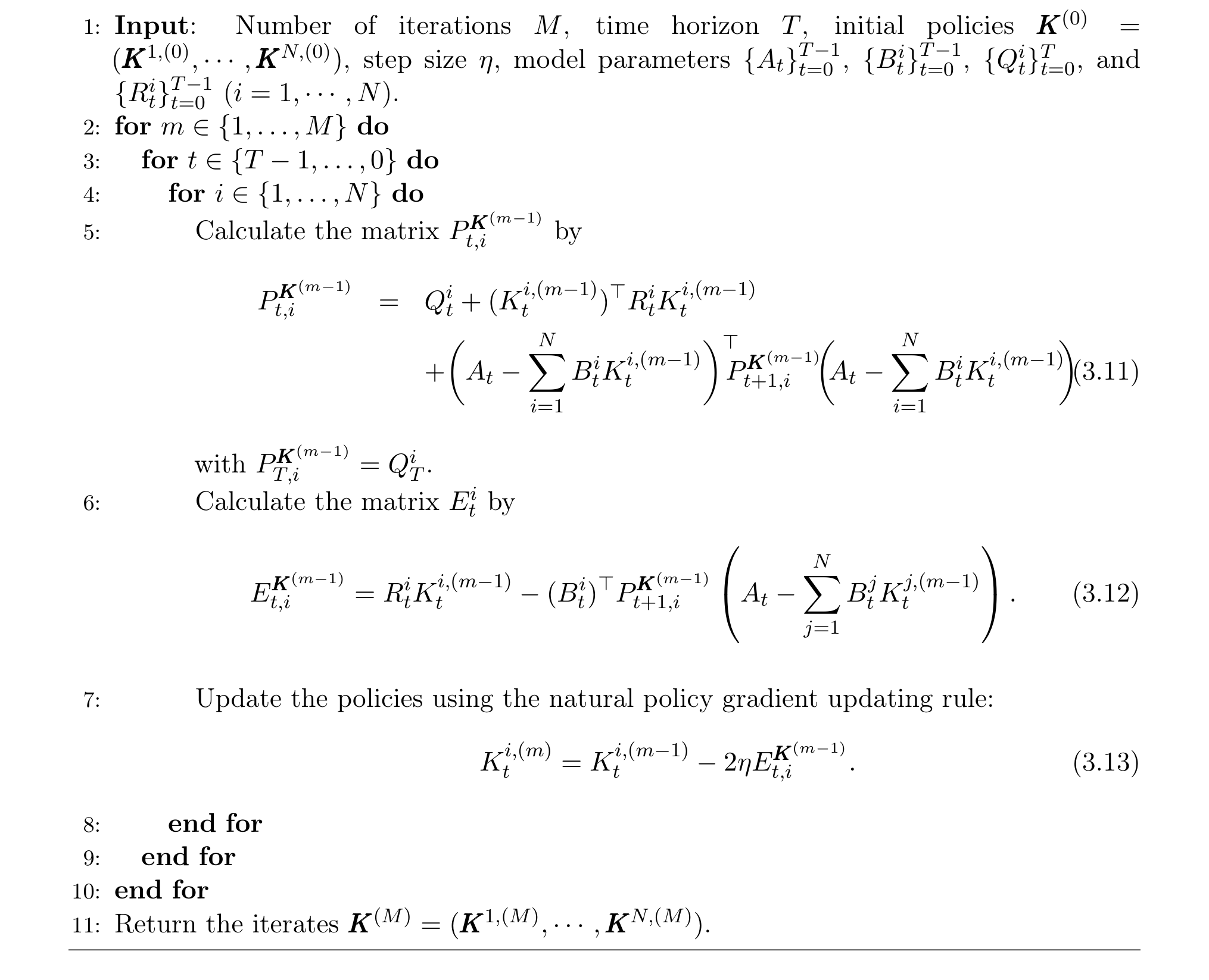
With access to the model parameters, players can directly calculate their own policy gradient and perform the natural policy gradient steps iteratively. See Algorithm 1 for the details. Unlike the nested-loop updates in some zero-sum LQ game settings (Zhang et al., 2021a, 2019) in which the inner-loop updates are sample inefficient, each player updates their policies simultaneously at each iteration in Algorithm 1. This simultaneous updating framework is a more realistic set-up for practical examples such as online auction bidding.
Equivalent Form of the Natural Policy Gradient. Following the explanation of the natural gradient method in the single-agent setting (Fazel et al., 2018), we provide an equivalent form of the natural gradient method with Fisher information in the game setting.
In our NNN-player game case, we assume player iii’s updating rule follows
where GKtiG_{K_t^i}GKti is the Fisher information matrix:
under a linear policy with additive Gaussian noise (Rajeswaran et al., 2017), in that
By a similar analysis to that in Fazel et al. (2018), we can show that the Fisher information matrix of size kid×kidk_id\times k_idkid×kid, which is indexed as [GKti](j,q),(j′,q′)[G_{K_t^i}]_{(j,q),(j',q')}[GKti](j,q),(j′,q′) where j,j′∈{1,2,…,ki}j,j'\in\{1,2,\ldots,k_i\}j,j′∈{1,2,…,ki} and q,q′∈{1,2,…,d}q,q'\in\{1,2,\ldots,d\}q,q′∈{1,2,…,d}, has a block diagonal form where the only non-zeros blocks are [GKti](j,⋅),(j,⋅)=ΣtK=E[xtK(xtK)⊤][G_{K_t^i}]_{(j,\cdot),(j,\cdot)}=\Sigma_t^K=\mathbb{E}[x_t^K(x_t^K)^\top][GKti](j,⋅),(j,⋅)=ΣtK=E[xtK(xtK)⊤] (this is the block corresponding to the iii-th coordinate of the action, as jjj ranges from 111 to kik_iki). Hence (3.6) is equivalent to the following updating rule
which is equivalent to (3.5).
Remark 4 In Algorithm 1, during iteration mmm, each player first calculates the solution to the backward Riccati equation in (3.11) based on the observations from the previous iteration m−1m-1m−1, and obtains the policy gradients in (3.12). The natural gradient method is then applied in (3.13) to update the policy for that iteration. Note that (3.13) does not involve (ΣtK)−1(\Sigma_t^K)^{-1}(ΣtK)−1 since, as we show later in Lemma 9, we have 2Et,iK=∇KtiCi(K)(ΣtK)−12E_{t,i}^K=\nabla_{K_t^i}C^i(K)(\Sigma_t^K)^{-1}2Et,iK=∇KtiCi(K)(ΣtK)−1.
A straightforward analysis shows that the computational complexity of Algorithm 1 is O(MNTmax(ki2d,d3))O(MNT\max(k_i^2d,d^3))O(MNTmax(ki2d,d3)) and that it requires (Td∑i=1Nki)(Td\sum_{i=1}^N k_i)(Td∑i=1Nki) storage units for KKK.
We now introduce the main assumption and the main result for the natural policy gradient method applied to the class of general-sum LQ games. To start we define ρ∗\rho^*ρ∗ as
for some small constant δ>0\delta>0δ>0, and define ψ:=maxi{Ci(Ki,(0),K−i∗)−Ci(K∗)}\psi:=\max_i\{C^i(K^{i,(0)},K^{-i*})-C^i(K^*)\}ψ:=maxi{Ci(Ki,(0),K−i∗)−Ci(K∗)}. Now set
Assumption 4 (System Noise) The system parameters satisfy the following inequality
Note that σX\sigma_XσX appears on both sides of (3.14) (indirectly through ρˉ\bar{\rho}ρˉ on the R.H.S., ΣK∗\Sigma^{K^*}ΣK∗ on the L.H.S., and terms involving costs CiC^iCi) and when σX\sigma_XσX increases, the LHS of (3.14) increases while the RHS of (3.14) decreases. Therefore, Assumption 4 requires σX\sigma_XσX to be large enough such that inequality (3.14) holds. This can be interpreted as ensuring that the system needs a certain level of noise for the learning agents to find the correct direction towards the Nash equilibrium. Assumption 4 also imposes conditions on the initial policy K(0)K(0)K(0) as ψ\psiψ depends on the difference between Ci(Ki,(0),K−i∗)C^i(K^{i,(0)},K^{-i*})Ci(Ki,(0),K−i∗) and Ci(K∗)C^i(K^*)Ci(K∗).
Below we provide two examples such that Assumption 4 is satisfied. In Section 5 we will show that, at least in some circumstances, the natural policy gradient method leads to the Nash equilibrium even when Assumption 4 is violated. This further demonstrates the power of the natural policy gradient method in practice.
3.1. Regularity of the LQ game and Properties of the Gradient Descent Dynamics
We begin with the analysis of some properties of the NNN-player general-sum LQ game (2.1)–(2.3). Our aim is to establish two key results, Lemma 11 and Lemma 12, which provide the gradient dominance condition and a smoothness condition on the cost function Ci(K)C^i(K)Ci(K) of player iii with respect to the joint policy KKK from all players, respectively.
In the finite horizon setting, define Pt,iKP_{t,i}^KPt,iK as the solution to
with terminal condition
Lemma 8 Assume Assumption 1 holds. Then for i=1,…,Ni=1,\ldots,Ni=1,…,N, t=0,…,Tt=0,\ldots,Tt=0,…,T the matrices Pt,iKP_{t,i}^KPt,iK defined in (3.25) are positive definite.
Proof We prove that the terms in the sequence {Pt,iK}t=0T\{P_{t,i}^K\}_{t=0}^{T}{Pt,iK}t=0T are positive definite for i=1,…,Ni=1,\ldots,Ni=1,…,N by backward induction. For t=Tt=Tt=T, PT,iK=QTiP_{T,i}^K=Q_T^iPT,iK=QTi is positive definite since QTiQ_T^iQTi is positive definite. Assume Pt+1,iKP_{t+1,i}^KPt+1,iK is positive definite for some t+1t+1t+1, then take any z∈Rdz\in\mathbb{R}^dz∈Rd such that z≠0z\ne0z=0,
The last inequality holds since z⊤Qtiz>0z^\top Q_t^iz>0z⊤Qtiz>0 and the other terms are non-negative under Assumption 1. By backward induction, we have Pt,iKP_{t,i}^KPt,iK positive definite, ∀t=0,1,…,T\forall t=0,1,\ldots,T∀t=0,1,…,T.
Player iii’s cost under the set of policies KKK can be rewritten as
where the expectation is taking with respect to the initial state x0x_0x0 and the Nt,iKN_{t,i}^KNt,iK are defined backwards:
To see this,
In addition, for t=0,1,…,T−1t=0,1,\ldots,T-1t=0,1,…,T−1 and i=1,…,Ni=1,\ldots,Ni=1,…,N, define
Then we have the following representation of the gradient terms.
Lemma 9 The policy gradients have the following representation: for t=0,1,…,T−1t=0,1,\ldots,T-1t=0,1,…,T−1,
Proof Expressing the cost function in terms of KtiK_t^iKti and suppressing the arguments of the cost ctic_t^icti,
Therefore, for i=1,…,Ni=1,\ldots,Ni=1,…,N, the gradients are given by
We can write the value function for player iii, VKi(x,t)V_K^i(x,t)VKi(x,t) for t=0,1,…,T−1t=0,1,\ldots,T-1t=0,1,…,T−1, as
with terminal condition
where Nt,iKN_{t,i}^KNt,iK is defined in (3.26), and Ew\mathbb{E}_wEw denotes the expectation over the noise www. We then define the QQQ function, QKi(x,u,t)Q_K^i(x,u,t)QKi(x,u,t) for the Markovian control u=(u1,…,uN)u=(u^1,\ldots,u^N)u=(u1,…,uN) to be
and the advantage function to be
Here Ewt\mathbb{E}_{w_t}Ewt denotes the expectation taken with respect to wtw_twt. Note that Ci(K)=E[VKi(x0,0)]C^i(K)=\mathbb{E}[V_K^i(x_0,0)]Ci(K)=E[VKi(x0,0)]. We write
and the control sequences under the policy (Ki0,K−i)(K^{i0},K^{-i})(Ki0,K−i) as {uti0,−i}t=0T−1\{u_t^{i0,-i}\}_{t=0}^{T-1}{uti0,−i}t=0T−1 with
where {xtKi0,K−i}t=0T\{x_t^{K^{i0},K^{-i}}\}_{t=0}^{T}{xtKi0,K−i}t=0T is the state trajectory under (Ki0,K−i)(K^{i0},K^{-i})(Ki0,K−i). Then we can write the difference between the cost functions of K=(K1,…,KN)K=(K^1,\ldots,K^N)K=(K1,…,KN) and (Ki0,K−i)(K^{i0},K^{-i})(Ki0,K−i) in terms of advantage functions.
Lemma 10 (Cost Difference) Assume KKK and (Ki0,K−i)(K^{i0},K^{-i})(Ki0,K−i) have finite costs. Then
where {uti0,−i}t=0T−1\{u_t^{i0,-i}\}_{t=0}^{T-1}{uti0,−i}t=0T−1 is defined in (3.30) with x0Ki0,K−i=xx_0^{K^{i0},K^{-i}}=xx0Ki0,K−i=x. For player iii,
Proof Write xt0=xtKi0,K−ix_t^0=x_t^{K^{i0},K^{-i}}xt0=xtKi0,K−i for simplicity and denote by cti0(x)c_t^{i0}(x)cti0(x) the (instantaneous) cost of player iii generated by (Ki0,K−i)(K^{i0},K^{-i})(Ki0,K−i) with a single trajectory starting from x00=xx_0^0=xx00=x. That is,
and
with
Therefore
where the third equality holds since cTi0(xT0)=VKi(xT0,T)c_T^{i0}(x_T^0)=V_K^i(x_T^0,T)cTi0(xT0)=VKi(xT0,T) by (3.29) with the same single trajectory.
For player iii, the advantage function is given by
Note that the derivations of Lemmas 8, 9 and 10 are largely inspired by Fazel et al. (2018) and Hambly et al. (2021). However, the final expressions are different since our setting is different from both Fazel et al. (2018) and Hambly et al. (2021). For completeness, we provide the proofs and derivations in our context.
For the policy gradient method (Fazel et al., 2018; Hambly et al., 2021) in the single-agent setting, gradient domination and smoothness of the objective function are two key conditions to guarantee the global convergence of the gradient descent methods. This is also the case for the NNN-player game setting. The gradient dominance condition for each player iii is proved in Lemma 11, which indicates that for a policy KKK, the distance between Ci(K)C^i(K)Ci(K) and the optimal cost Ci(K∗)C^i(K^*)Ci(K∗) is bounded by the sum of the magnitudes of the gradients ∇tCi(K)\nabla_t C^i(K)∇tCi(K) for t=0,1,…,T−1t=0,1,\ldots,T-1t=0,1,…,T−1. The smoothness condition for each player iii is proved in Lemma 12 where the difference between Ci(Ki0,K−i)C^i(K^{i0},K^{-i})Ci(Ki0,K−i) and Ci(K)C^i(K)Ci(K) can be rewritten as a function of Ki0−KiK^{i0}-K^iKi0−Ki.
Lemma 11 (Gradient Dominance) Assume Assumptions 1, 2, and 3 hold. Then, for player iii, we have
and
Proof By Lemma 10, we have
with equality in the last line when Kti0=Kti−(Rti+(Bti)⊤Pt+1,iKBti)−1Et,iKK_t^{i0}=K_t^i-(R_t^i+(B_t^i)^\top P_{t+1,i}^KB_t^i)^{-1}E_{t,i}^KKti0=Kti−(Rti+(Bti)⊤Pt+1,iKBti)−1Et,iK. Then, by Lemma 10, letting {xt∗}t=0T\{x_t^*\}_{t=0}^{T}{xt∗}t=0T and ut∗=(ut1∗,…,utN∗)u_t^*=(u_t^{1*},\ldots,u_t^{N*})ut∗=(ut1∗,…,utN∗) with uti∗=−Kti∗xt∗u_t^{i*}=-K_t^{i*}x_t^*uti∗=−Kti∗xt∗ denote the state and control sequences induced by the set of optimal policies K∗K^*K∗, we have
Note that (3.32) holds as Tr(AB)≤σmax(A)Tr(B)\operatorname{Tr}(AB)\le\sigma_{\max}(A)\operatorname{Tr}(B)Tr(AB)≤σmax(A)Tr(B) for any matrix AAA and real symmetric positive semi-definite matrices BBB of the same size (Saniuk and Rhodes, 1987). By Lemma 1 in Wang et al. (1986), for any symmetric matrix AAA and any symmetric positive semi-definite matrix BBB, it holds that
These bounds will be used in several places. For the lower bound, consider Kti0=Kti−(Rti+(Bti)⊤Pt+1,iKBti)−1Et,iKK_t^{i0}=K_t^i-(R_t^i+(B_t^i)^\top P_{t+1,i}^KB_t^i)^{-1}E_{t,i}^KKti0=Kti−(Rti+(Bti)⊤Pt+1,iKBti)−1Et,iK. Using Ci(Ki0,K−i∗)≥Ci(K∗)C^i(K^{i0},K^{-i*})\ge C^i(K^*)Ci(Ki0,K−i∗)≥Ci(K∗) and letting {utKi0,K−i∗}t=0T−1\{u_t^{K^{i0},K^{-i*}}\}_{t=0}^{T-1}{utKi0,K−i∗}t=0T−1 denote the control sequence induced by (Ki0,K−i∗)(K^{i0},K^{-i*})(Ki0,K−i∗), by Lemma 10 we have
As in the single-agent case (Fazel et al., 2018; Hambly et al., 2021), we now provide an expression for Ci(Ki0,K−i)−Ci(K)C^i(K^{i0},K^{-i})-C^i(K)Ci(Ki0,K−i)−Ci(K), which is easier to analyze.
Lemma 12 (Almost Smoothness) For two sets of policies KKK and (Ki0,K−i)(K^{i0},K^{-i})(Ki0,K−i), we have that
Proof By Lemma 10,
Lemma 13 Assume Assumptions 1 and 2 hold. Then for t=0,1,…,Tt=0,1,\ldots,Tt=0,1,…,T and i=1,…,Ni=1,\ldots,Ni=1,…,N,
Proof By the trace inequality (3.33), it is straightforward to see that
and
Then the statements in Lemma 13 follow since under Assumptions 1 and 2, we have σX>0\sigma_X>0σX>0 and σQ>0\sigma_Q>0σQ>0.
3.2. Perturbation Analysis of the State Covariance Matrix
Our aim in this section is to provide an explicit control of the change in the state covariance matrix after a change in policy KiK^iKi. We begin by defining two linear operators on symmetric matrices. For X∈Rd×dX\in\mathbb{R}^{d\times d}X∈Rd×d we set
and
If we write GtK=FtK∘Ft−1K∘⋯∘F0KG_t^K=F_t^K\circ F_{t-1}^K\circ\cdots\circ F_0^KGtK=FtK∘Ft−1K∘⋯∘F0K, then the following relationships hold:
and
When the policy KKK is clear we will write Gt=GtKG_t=G_t^KGt=GtK and Ft=FtKF_t=F_t^KFt=FtK. We also define the induced norm for these operators as
where T=FtK,GtK,TKT=F_t^K,G_t^K,T_KT=FtK,GtK,TK and the supremum is over all symmetric matrix XXX with non-zero spectral norm.
We first show the relationship between the operator TKT_KTK and the quantity ΣK\Sigma^KΣK.
Proposition 1 For T≥2T\ge2T≥2, we have that
where
with Dt,s=∏u=st(Au−∑j=1NBujKuj)D_{t,s}=\prod_{u=s}^{t}(A_u-\sum_{j=1}^{N}B_u^jK_u^j)Dt,s=∏u=st(Au−∑j=1NBujKuj) (for s=1,2,…,ts=1,2,\ldots,ts=1,2,…,t), and Σ0=E[x0x0⊤]\Sigma_0=\mathbb{E}[x_0x_0^\top]Σ0=E[x0x0⊤].
Proof Recall that ΣtK=E[xtxt⊤]\Sigma_t^K=\mathbb{E}[x_tx_t^\top]ΣtK=E[xtxt⊤] and note that
We first prove that for t=2,3,…,Tt=2,3,\ldots,Tt=2,3,…,T,
We have the result for t=1t=1t=1, so assume (3.39) holds for t≤kt\le kt≤k. Then for t=k+1t=k+1t=k+1,
Therefore (3.39) holds, ∀t=1,2,…,T\forall t=1,2,\ldots,T∀t=1,2,…,T. Finally,
Given two policies KKK and K0=(K10,…,KN0)K^0=(K^{10},\ldots,K^{N0})K0=(K10,…,KN0), let us define
for some small constant ξ>0\xi>0ξ>0.
For any given policy KKK, max0≤t≤T−1∥At−∑j=1NBtjKtj∥\max_{0\le t\le T-1}\|A_t-\sum_{j=1}^{N}B_t^jK_t^j\|max0≤t≤T−1∥At−∑j=1NBtjKtj∥ measures the radius of the state dynamics under policy KKK. Thus ρK,K0\rho_{K,K^0}ρK,K0 defined in (3.40) is the maximum radius of the policies KKK, (Ki,K−i∗)(K^i,K^{-i*})(Ki,K−i∗), (Ki0,K−i∗)(K^{i0},K^{-i*})(Ki0,K−i∗), and (Ki0,K−i)(K^{i0},K^{-i})(Ki0,K−i) (i=1,2,…,Ni=1,2,\ldots,Ni=1,2,…,N). We will show later that the value (or the upper bound) of ρK,K0\rho_{K,K^0}ρK,K0 plays an essential role in the convergence analysis.
Remark 14 By the definition of ρK,K0\rho_{K,K^0}ρK,K0 in (3.40), we have ρK,K0≥1+ξ>1\rho_{K,K^0}\ge1+\xi>1ρK,K0≥1+ξ>1. This regularization term 1+ξ1+\xi1+ξ is introduced to simplify the presentation. Alternatively, if we remove this term from the definition of ρK,K0\rho_{K,K^0}ρK,K0, a similar analysis can still be carried out by considering the different cases: ρK,K0<1\rho_{K,K^0}<1ρK,K0<1, ρK,K0=1\rho_{K,K^0}=1ρK,K0=1 and ρK,K0>1\rho_{K,K^0}>1ρK,K0>1.
We now provide an upper bound for ρK,K0\rho_{K,K^0}ρK,K0.
Lemma 15 Assume Assumption 3 holds. Then,
where ρ∗\rho^*ρ∗ was defined in (3.9).
Proof By Lemma 12, we have
where (3.42) holds by the Cauchy-Schwarz inequality. Then we have
where (3.43) holds by (3.42). Also, by the triangle inequality we have
and
Finally, applying (3.42),
Therefore combining (3.43)–(3.46), we obtain the statement (3.41).
Recall the definition of Ft=FtKF_t=F_t^KFt=FtK and Gt=GtKG_t=G_t^KGt=GtK in (3.34) and (3.35) associated with KKK. Similarly let us define Gti0=FtKi0,K−i∘Ft−1Ki0,K−i∘⋯∘F0Ki0,K−iG_t^{i0}=F_t^{K^{i0},K^{-i}}\circ F_{t-1}^{K^{i0},K^{-i}}\circ\cdots\circ F_0^{K^{i0},K^{-i}}Gti0=FtKi0,K−i∘Ft−1Ki0,K−i∘⋯∘F0Ki0,K−i for the set of policies (Ki0,K−i)(K^{i0},K^{-i})(Ki0,K−i) and write Fti0=FtKi0,K−iF_t^{i0}=F_t^{K^{i0},K^{-i}}Fti0=FtKi0,K−i. We now establish a perturbation analysis for FtF_tFt and GtG_tGt.
Lemma 16 For all t=0,1,…,T−1t=0,1,\ldots,T-1t=0,1,…,T−1, we have
Proof For player iii,
By (3.37) the operator norm of Ft−Fti0F_t-F_t^{i0}Ft−Fti0 is the maximum possible ratio of ∥(Ft−Fti0)(X)∥\|(F_t-F_t^{i0})(X)\|∥(Ft−Fti0)(X)∥ and ∥X∥\|X\|∥X∥. Then letting Y=At−∑j=1NBtjKtjY=A_t-\sum_{j=1}^{N}B_t^jK_t^jY=At−∑j=1NBtjKtj and Z=At−BtiKti0−∑j=1j≠iNBtjKtjZ=A_t-B_t^iK_t^{i0}-\sum_{\substack{j=1\\j\ne i}}^NB_t^jK_t^jZ=At−BtiKti0−∑j=1j=iNBtjKtj in
and using the norm bound ∥AX∥≤∥A∥∥X∥\|AX\|\le\|A\|\|X\|∥AX∥≤∥A∥∥X∥, we have
Therefore we obtain the statement ∥Ft−Fti0∥≤2ρK,K0γB∥Kti−Kti0∥\|F_t-F_t^{i0}\|\le2\rho_{K,K^0}\gamma_B\|K_t^i-K_t^{i0}\|∥Ft−Fti0∥≤2ρK,K0γB∥Kti−Kti0∥.
Recall that FtF_tFt and GtG_tGt are defined in equations (3.34) and (3.35). Then we have the following lemma on perturbation analysis for GtG_tGt.
Lemma 17 (Perturbation Analysis for GtG_tGt) For any symmetric matrix Σ∈Rd×d\Sigma\in\mathbb{R}^{d\times d}Σ∈Rd×d and i=1,…,Ni=1,\ldots,Ni=1,…,N, we have that
Proof By direct calculation,
Then for any symmetric matrix Σ∈Rd×d\Sigma\in\mathbb{R}^{d\times d}Σ∈Rd×d and t≥0t\ge0t≥0,
Therefore,
As it is a geometric series, summing (3.50) over t∈{0,1,2,…,T−2}t\in\{0,1,2,\ldots,T-2\}t∈{0,1,2,…,T−2} with ∥G0i0−G0∥=∥F0i0−F0∥\|G_0^{i0}-G_0\|=\|F_0^{i0}-F_0\|∥G0i0−G0∥=∥F0i0−F0∥, gives
Recall that γA\gamma_AγA, γB\gamma_BγB, and γR\gamma_RγR are defined in (3.4). Then we have the following perturbation analysis of ΣK\Sigma^KΣK.
Lemma 18 (Perturbation Analysis of ΣK\Sigma^KΣK) Assume Assumption 1 holds. Then
Proof Using Lemma 16,
Define Dt,si0=∏u=st(Au−BuiKui0−∑j=1j≠iNBujKuj)D_{t,s}^{i0}=\prod_{u=s}^{t}(A_u-B_u^iK_u^{i0}-\sum_{\substack{j=1\\j\ne i}}^NB_u^jK_u^j)Dt,si0=∏u=st(Au−BuiKui0−∑j=1j=iNBujKuj) (for s=1,2,…,ts=1,2,\ldots,ts=1,2,…,t). Then, in a similar way to the proof of Lemma 17, we have, ∀t=1,…,T−1\forall t=1,\ldots,T-1∀t=1,…,T−1,
By Proposition 1, (3.36) and (3.51), we have
The last inequality holds since ∥Σ0∥≤∥ΣKi,K−i∗∥≤Ci(Ki,K−i∗)/σQ\|\Sigma_0\|\le\|\Sigma^{K^i,K^{-i*}}\|\le C^i(K^i,K^{-i*})/\sigma_Q∥Σ0∥≤∥ΣKi,K−i∗∥≤Ci(Ki,K−i∗)/σQ by Lemma 13.
3.3. Convergence and Complexity Analysis
We are now in a position to provide the proof of our main Theorem 6. This will follow from two important lemmas. First, define
Further define g1g_1g1 and g2g_2g2 as follows
and
We also write Ci,−i∗=Ci(Ki,K−i∗)C^{i,-i*}=C^i(K^i,K^{-i*})Ci,−i∗=Ci(Ki,K−i∗), Ci∗=Ci(K∗)C^{i*}=C^i(K^*)Ci∗=Ci(K∗) and Ci0,−i∗=Ci(Ki0,K−i∗)C^{i0,-i*}=C^i(K^{i0},K^{-i*})Ci0,−i∗=Ci(Ki0,K−i∗) to simplify notation.
Lemma 19 (One-step Contraction) Assume Assumptions 1, 2, and 3 hold, and that
Also assume the policy update step for player iii at time ttt is given by
where
with
Let α:=σXg1−g2/σX4>0\alpha:=\sigma_Xg_1-g_2/\sigma_X^4>0α:=σXg1−g2/σX4>0. Then, we have:
- η∈(0,1α)\eta\in(0,\frac{1}{\alpha})η∈(0,α1); and
- the following inequality holds
Remark 20 (1) In the one-step contraction analysis (Lemma 19), (3.56) imposes a condition on C(Ki,K−i∗)C(K^i,K^{-i*})C(Ki,K−i∗) which is associated with the current policy KKK. In the analysis of the global convergence result (Theorem 6), (3.14) imposes a similar condition on C(Ki,(0),K−i∗)C(K^{i,(0)},K^{-i*})C(Ki,(0),K−i∗) which is associated with the initial policy K(0)K^{(0)}K(0). Condition (3.14) in Assumption 4 and the step size condition in Theorem 6 guarantee that condition (3.56) holds for any K=K(m)K=K^{(m)}K=K(m) throughout the training process (m=1,2,…,Mm=1,2,\ldots,Mm=1,2,…,M). This further ensures that the one-step contraction analysis in Lemma 19 can be applied iteratively which leads to the global convergence result as stated in Theorem 6.
(2) Note that the numbers such as 20 and 80 that appear in I1,I2I_1,I_2I1,I2 are not arbitrary and, although some minor improvements can be made by optimizing at various stages, they enable us to obtain reasonable bounds.
Proof We break this proof up into a series of steps.
Step 1: We first consider the consequences of the condition η≤min{I1,I2}\eta\le\min\{I_1,I_2\}η≤min{I1,I2}. Straightforward calculations show that when condition η≤I1\eta\le I_1η≤I1 is satisfied, the following inequalities hold:
- ∀i=1,…,N\forall i=1,\ldots,N∀i=1,…,N,
- ∀i=1,…,N\forall i=1,\ldots,N∀i=1,…,N,
- ∀i=1,…,N\forall i=1,\ldots,N∀i=1,…,N,
In the case where η≤I2\eta\le I_2η≤I2, we have ∀i=1,…,N\forall i=1,\ldots,N∀i=1,…,N
By (3.60) and Lemma 13 we have
Therefore, we have ρK,K0≤ρK\rho_{K,K^0}\le\rho_KρK,K0≤ρK by Lemma 15.
Step 2: We bound the norm of the state covariance matrix. By Lemma 16,
and hence by Lemma 18, we have
where the last inequality holds by (3.61) when ∑t=0T−1∥∇KtiCi(K)∥>0\sum_{t=0}^{T-1}\|\nabla_{K_t^i}C^i(K)\|>0∑t=0T−1∥∇KtiCi(K)∥>0. Note that when ∑t=0T−1∥∇KtiCi(K)∥=0\sum_{t=0}^{T-1}\|\nabla_{K_t^i}C^i(K)\|=0∑t=0T−1∥∇KtiCi(K)∥=0, we have ∥ΣKi,K−i∗−ΣKi0,K−i∗∥=0<σX/10\|\Sigma^{K^i,K^{-i*}}-\Sigma^{K^{i0},K^{-i*}}\|=0<\sigma_X/10∥ΣKi,K−i∗−ΣKi0,K−i∗∥=0<σX/10 and hence (3.64) still holds in this case. Therefore, by Lemma 13, and noting σX≤∥ΣKi0,K−i∗∥/T\sigma_X\le\|\Sigma^{K^{i0},K^{-i*}}\|/TσX≤∥ΣKi0,K−i∗∥/T,
which leads to
Step 3: We now bound ∥Pt,iK−Pt,iKi,K−i∗∥\|P_{t,i}^K-P_{t,i}^{K^i,K^{-i*}}\|∥Pt,iK−Pt,iKi,K−i∗∥ by ∑j=1,j≠iN∥Kj−Kj∗∥\sum_{j=1,j\ne i}^{N}\|K^j-K^{j*}\|∑j=1,j=iN∥Kj−Kj∗∥ where K=(Ki,K−i)K=(K^i,K^{-i})K=(Ki,K−i).
where the last inequality holds by letting X=Pt+1,iKi,K−i∗X=P_{t+1,i}^{K^i,K^{-i*}}X=Pt+1,iKi,K−i∗, Y=At−∑j=1NBtjKtjY=A_t-\sum_{j=1}^{N}B_t^jK_t^jY=At−∑j=1NBtjKtj, and Z=At−BtiKti−∑j=1j≠iNBtjKtj∗Z=A_t-B_t^iK_t^i-\sum_{\substack{j=1\\j\ne i}}^NB_t^jK_t^{j*}Z=At−BtiKti−∑j=1j=iNBtjKtj∗ in (3.48). Since ∥PT,iK−PT,iKi,K−i∗∥=0\|P_{T,i}^K-P_{T,i}^{K^i,K^{-i*}}\|=0∥PT,iK−PT,iKi,K−i∗∥=0 holds at terminal time TTT, we obtain ∀t=0,…,T−1\forall t=0,\ldots,T-1∀t=0,…,T−1,
Therefore, ∀t=0,1,…,T−1\forall t=0,1,\ldots,T-1∀t=0,1,…,T−1,
Step 4: We can now estimate the cost difference between using KiK^iKi and the update Ki0K^{i0}Ki0. By Lemma 12 we have
Using the updating rule Kti0=Kti−η∇KtiCi(K)(ΣtK)−1K_t^{i0}=K_t^i-\eta\nabla_{K_t^i}C^i(K)(\Sigma_t^K)^{-1}Kti0=Kti−η∇KtiCi(K)(ΣtK)−1 and the expression for the gradient from Lemma 9,
Now, letting ω2=2/σX\omega^2=2/\sigma_Xω2=2/σX in 2Tr(A⊤B)=Tr(A⊤B+B⊤A)≤ω2Tr(A⊤A)+1ω2Tr(B⊤B)2\operatorname{Tr}(A^\top B)=\operatorname{Tr}(A^\top B+B^\top A)\le\omega^2\operatorname{Tr}(A^\top A)+\frac{1}{\omega^2}\operatorname{Tr}(B^\top B)2Tr(A⊤B)=Tr(A⊤B+B⊤A)≤ω2Tr(A⊤A)+ω21Tr(B⊤B), which holds for any matrices AAA and BBB of the same dimension, we have
Now, using ∥ΣKi0,K−i∗∥≤2Ci,−i∗/σQ\|\Sigma^{K^{i0},K^{-i*}}\|\le2C^{i,-i*}/\sigma_Q∥ΣKi0,K−i∗∥≤2Ci,−i∗/σQ by (3.66) (this is a loose approximation in order to ease the analysis and smooth out the presentation), we can bound the step size condition in (3.62) by
This gives
Hence, using this in (3.72), we have
where
Therefore, by (3.66), (3.71), Lemma 11, and Lemma 13,
where
Step 5: Finally we can establish the one-step contraction. Using (3.74), we have
Hence by Lemma 12 and (3.42), we have
and thus
Summing up (3.77) for i=1,…,Ni=1,\ldots,Ni=1,…,N, we have
Since η≤I2\eta\le I_2η≤I2, we have (3.63) and then
and hglob≤hˉglobh_{\mathrm{glob}}\le\bar{h}_{\mathrm{glob}}hglob≤hˉglob, where hˉglob\bar{h}_{\mathrm{glob}}hˉglob is given by
Under condition (3.56), we have
which indicates that αη>0\alpha\eta>0αη>0. Since η≤1/σR\eta\le1/\sigma_Rη≤1/σR, we have
Recall that in the statement we define α=σXg1−g2/σX4\alpha=\sigma_Xg_1-g_2/\sigma_X^4α=σXg1−g2/σX4. Therefore we have αη<1\alpha\eta<1αη<1. Along with (3.78), we obtain the one-step contraction (3.59).
Lemma 21 Assume Assumptions 1, 2, and 3 hold. Then we have that for player iii,
Proof Using Lemma 9, we have
and
By (3.42), (3.71), we have
By Lemma 11 and Lemma 13, we have
By Proposition 1,
Note that here we use ∑t=1T−1∑s=1tρK2(t−s)≤T∑s=1T−1ρK2(T−s)\sum_{t=1}^{T-1}\sum_{s=1}^{t}\rho_K^{2(t-s)}\le T\sum_{s=1}^{T-1}\rho_K^{2(T-s)}∑t=1T−1∑s=1tρK2(t−s)≤T∑s=1T−1ρK2(T−s), which is a loose bound in order to simplify the presentation. Therefore, combining (3.81)–(3.85), we obtain the statement (3.80).
Finally, we are ready to provide the proof for the main result based on Lemmas 19 and 21.
Proof [Proof of Theorem 6] We first show that the total cost for the NNN players decreases at round m=1m=1m=1. Take K=K(0)K=K^{(0)}K=K(0) and K0=K(1)K^0=K^{(1)}K0=K(1) in Lemma 19, we begin by showing that there exists a positive lower bound on the RHS of (3.58). By the Cauchy-Schwarz inequality and Lemma 21,
where the last inequality holds since, after performing one-step natural policy gradient
Kti,(1)=Kti,(0)−η∇KtiCi(K(0))(ΣtK(0))−1K_t^{i,(1)}=K_t^{i,(0)}-\eta\nabla_{K_t^i}C^i(K^{(0)})(\Sigma_t^{K^{(0)}})^{-1}Kti,(1)=Kti,(0)−η∇KtiCi(K(0))(ΣtK(0))−1, we have
where ρ∗\rho^*ρ∗ and ρˉ\bar{\rho}ρˉ are defined in (3.9) and (3.10), and ψ:=maxi{Ci(Ki,(0),K−i∗)−Ci∗}\psi:=\max_i\{C^i(K^{i,(0)},K^{-i*})-C^{i*}\}ψ:=maxi{Ci(Ki,(0),K−i∗)−Ci∗}. (3.86) holds by Lemma 15.
Now we aim to show that 1/ρˉ1/\bar{\rho}1/ρˉ is bounded below by polynomials in some model parameters. Given that
and that Lemma 15, ρˉ\bar{\rho}ρˉ can be bounded above by polynomials in TTT, NNN, γA\gamma_AγA, γB\gamma_BγB, 1/σX1/\sigma_X1/σX, 1/σR1/\sigma_R1/σR, and ∥∣∣K∗∥∣∣\|||K^*\|||∥∣∣K∗∥∣∣, or a constant 1+ξ1+\xi1+ξ. Therefore, along with the fact that 1/d>1/((a+1)(b+1)(c+1))1/d>1/((a+1)(b+1)(c+1))1/d>1/((a+1)(b+1)(c+1)) for d<ab+cd<ab+cd<ab+c with some a,b,c,d>0a,b,c,d>0a,b,c,d>0 and 1/an+1>1/(a+1)n1/a^{n+1}>1/(a+1)^n1/an+1>1/(a+1)n for a>0a>0a>0 and n∈N+n\in\mathbb{N}^+n∈N+, 1/ρˉ1/\bar{\rho}1/ρˉ is bounded below by polynomials in 1/(T+1)1/(T+1)1/(T+1), 1/(N+1)1/(N+1)1/(N+1), 1/(γA+1)1/(\gamma_A+1)1/(γA+1), 1/(γB+1)1/(\gamma_B+1)1/(γB+1), σX\sigma_XσX, 1/(σX+1)1/(\sigma_X+1)1/(σX+1), σR\sigma_RσR, 1/(σR+1)1/(\sigma_R+1)1/(σR+1), and 1/(∥∣∣K∗∥∣∣+1)1/(\|||K^*\|||+1)1/(∥∣∣K∗∥∣∣+1), or a constant 1/(1+ξ)1/(1+\xi)1/(1+ξ). Similarly, I1I_1I1 can be bounded below by polynomials in 1/(d+1)1/(d+1)1/(d+1), 1/(N+1)1/(N+1)1/(N+1), 1/(T+1)1/(T+1)1/(T+1), 1/(∑i=1NCi,−i∗+1)1/(\sum_{i=1}^{N}C^{i,-i*}+1)1/(∑i=1NCi,−i∗+1), 1/(∥W∥+1)1/(\|W\|+1)1/(∥W∥+1), 1/(∥Σ0∥+1)1/(\|\Sigma_0\|+1)1/(∥Σ0∥+1), 1/(γA+1)1/(\gamma_A+1)1/(γA+1), 1/(γB+1)1/(\gamma_B+1)1/(γB+1), 1/(γR+1)1/(\gamma_R+1)1/(γR+1), 1/(σR+1)1/(\sigma_R+1)1/(σR+1), σR\sigma_RσR, 1/(σQ+1)1/(\sigma_Q+1)1/(σQ+1), σQ\sigma_QσQ, 1/(σX+1)1/(\sigma_X+1)1/(σX+1), σX\sigma_XσX, and 1/(∥∣∣K∗∥∣∣+1)1/(\|||K^*\|||+1)1/(∥∣∣K∗∥∣∣+1); and I2I_2I2 can be bounded below by polynomials in 1/(∑iki+1)1/(\sum_i k_i+1)1/(∑iki+1), 1/(d+1)1/(d+1)1/(d+1), ddd, 1/(∑i=1NCi,−i∗+1)1/(\sum_{i=1}^{N}C^{i,-i*}+1)1/(∑i=1NCi,−i∗+1), 1/(γB+1)1/(\gamma_B+1)1/(γB+1), 1/(σQ+1)1/(\sigma_Q+1)1/(σQ+1), σQ\sigma_QσQ, 1/(γR+1)1/(\gamma_R+1)1/(γR+1), 1/(σX+1)1/(\sigma_X+1)1/(σX+1), σX\sigma_XσX.
Hence, there exists η0∈H(∑i=1NCi(Ki,(0),K−i∗)+1)\eta_0\in\mathcal{H}\left(\sum_{i=1}^{N}C^i(K^{i,(0)},K^{-i*})+1\right)η0∈H(∑i=1NCi(Ki,(0),K−i∗)+1) as an appropriate polynomial in ∑i=1NCi(Ki,(0),K−i∗)+1\sum_{i=1}^{N}C^i(K^{i,(0)},K^{-i*})+1∑i=1NCi(Ki,(0),K−i∗)+1, ∑iki+1\sum_i k_i+1∑iki+1, 1/(d+1)1/(d+1)1/(d+1), ddd, 1/(N+1)1/(N+1)1/(N+1), 1/(T+1)1/(T+1)1/(T+1), 1/(∥W∥+1)1/(\|W\|+1)1/(∥W∥+1), 1/(∥Σ0∥+1)1/(\|\Sigma_0\|+1)1/(∥Σ0∥+1), 1/(γA+1)1/(\gamma_A+1)1/(γA+1), 1/(γB+1)1/(\gamma_B+1)1/(γB+1), 1/(γR+1)1/(\gamma_R+1)1/(γR+1), 1/(σX+1)1/(\sigma_X+1)1/(σX+1), σX\sigma_XσX, 1/(σR+1)1/(\sigma_R+1)1/(σR+1), σR\sigma_RσR, 1/(σQ+1)1/(\sigma_Q+1)1/(σQ+1), σQ\sigma_QσQ, and 1/(∥∣∣K∗∥∣∣+1)1/(\|||K^*\|||+1)1/(∥∣∣K∗∥∣∣+1), such that when η<η0\eta<\eta_0η<η0, the step size condition (3.58) is satisfied. Therefore, by Lemma 19, we have
with α\alphaα defined in (3.20), which implies the total cost of NNN players decreases at m=1m=1m=1. Proceeding inductively, assume the following facts hold at round mmm:
- Ci(Ki,(m−1),K−i∗)−Ci∗≤ψC^i(K^{i,(m-1)},K^{-i*})-C^{i*}\le\psiCi(Ki,(m−1),K−i∗)−Ci∗≤ψ for i=1,2,…,Ni=1,2,\ldots,Ni=1,2,…,N;
- ρK(m−1)≤ρˉ\rho_{K^{(m-1)}}\le\bar{\rho}ρK(m−1)≤ρˉ;
- ∑i=1N(Ci(Ki,(m),K−i∗)−Ci∗)≤(1−αη)∑i=1N(Ci(Ki,(m−1),K−i∗)−Ci∗)\sum_{i=1}^{N}(C^i(K^{i,(m)},K^{-i*})-C^{i*})\le(1-\alpha\eta)\sum_{i=1}^{N}(C^i(K^{i,(m-1)},K^{-i*})-C^{i*})∑i=1N(Ci(Ki,(m),K−i∗)−Ci∗)≤(1−αη)∑i=1N(Ci(Ki,(m−1),K−i∗)−Ci∗).
Now we prove the above facts also hold in round m+1m+1m+1. Taking K=K(m−1)K=K^{(m-1)}K=K(m−1) and K0=K(m)K^0=K^{(m)}K0=K(m) in (3.77), we have
The last inequality holds since 1−ησXσR∥ΣK∗∥+ηhglobT(N−1)2σXσR<11-\eta\frac{\sigma_X\sigma_R}{\|\Sigma^{K^*}\|}+\eta h_{\mathrm{glob}}\frac{T(N-1)^2}{\sigma_X\sigma_R}<11−η∥ΣK∗∥σXσR+ηhglobσXσRT(N−1)2<1 under Assumption 4. Therefore by (3.53), we have
Thus the step size condition (3.58) is still satisfied for K=K(m)K=K^{(m)}K=K(m) and K0=K(m+1)K^0=K^{(m+1)}K0=K(m+1) with η<η0\eta<\eta_0η<η0, since ρK(m)≤ρˉ\rho_{K^{(m)}}\le\bar{\rho}ρK(m)≤ρˉ and ∑i=1NCi(Ki,(m),K−i∗)≤∑i=1NCi(Ki,(0),K−i∗)\sum_{i=1}^{N}C^i(K^{i,(m)},K^{-i*})\le\sum_{i=1}^{N}C^i(K^{i,(0)},K^{-i*})∑i=1NCi(Ki,(m),K−i∗)≤∑i=1NCi(Ki,(0),K−i∗). Therefore, Lemma 19 can be applied again for the update at round m+1m+1m+1 with K=K(m)K=K^{(m)}K=K(m) and K0=K(m+1)K^0=K^{(m+1)}K0=K(m+1) to obtain:
For ϵ>0\epsilon>0ϵ>0, provided
we have ∑i=1N(Ci(Ki,(M),K−i∗)−Ci∗)≤ϵ\sum_{i=1}^{N}(C^i(K^{i,(M)},K^{-i*})-C^{i*})\le\epsilon∑i=1N(Ci(Ki,(M),K−i∗)−Ci∗)≤ϵ.
4. The Natural Policy Gradient Method with Unknown Parameters
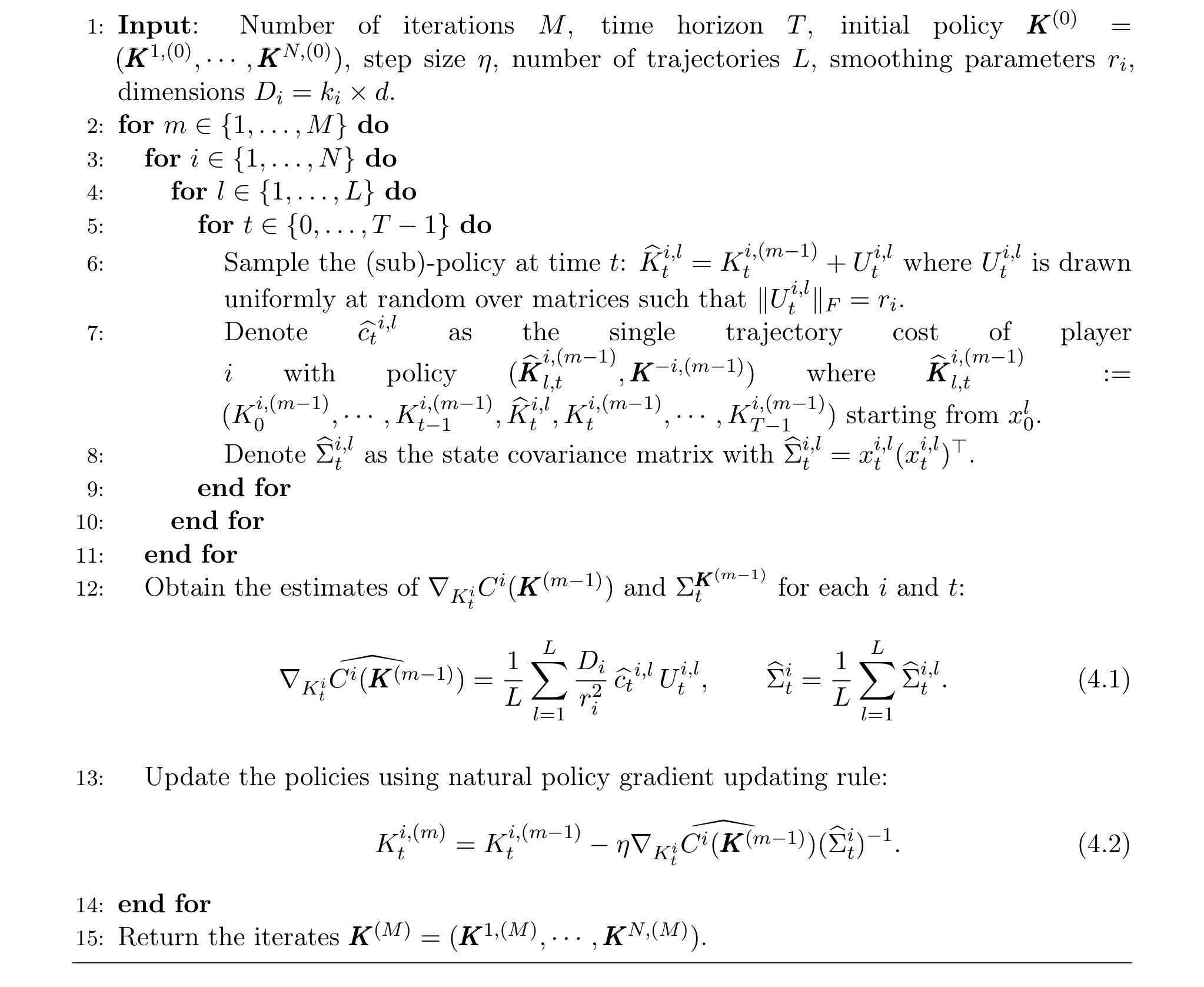
Based on the update rule in (3.5), it is straightforward to develop a model-free version of the natural policy gradient algorithm using sampled data. See Algorithm 2 for the natural policy gradient method with unknown parameters. In contrast to the model-based case, where the gradient ∇Ci(K)\nabla C^i(K)∇Ci(K) and covariance matrix Σti\Sigma_t^iΣti can be calculated directly, these two terms cannot be calculated in the model-free setting since the model parameters are unknown. Therefore, we propose to use a zeroth-order optimization method to estimate the gradient and an empirical covariance matrix to estimate the covariance matrix (see Equation 4.1). Building upon the theories in Section 3, high-probability convergence guarantees (linear convergence rate and polynomial sample complexity) for the model-free counterpart can be established in the same way as for the Linear Quadratic Regulator setting in Hambly et al. (2021).
5. Numerical Experiments
We demonstrate the performance of the natural policy gradient algorithms with three general-sum game examples. We will specifically focus on the following questions:
- In practice, how fast do the natural policy gradient algorithms converge to the true solution? How sensitive is the natural policy gradient algorithm to the step size and the initial policy?
- Do natural gradient methods converge when Assumption 4 is violated? How restrictive is Assumption 4 in practice?
- Can Theorem 6 provide any guidance on hyper-parameter tuning? In particular, does adding system noise improve the convergence?
The first example is a modified example from Mazumdar et al. (2020a), in which they show that in the setting of infinite time horizon and deterministic dynamics, the (vanilla) policy gradient algorithms have no guarantees of even local convergence to the Nash equilibria with known parameters. We will show in Section 5.1 that, under the same experimental set-up but over a finite time horizon with stochastic dynamics, the natural policy gradient algorithm with known parameters finds the Nash equilibrium with properly chosen initial policies and step sizes. The second example is a two-player LQ game with synthetic data (see Section 5.2). We will show that the system noise helps the natural policy gradient algorithm with unknown parameters to converge to the Nash equilibrium. Finally, we investigate the algorithm’s performance with known and unknown parameters for a three-player game example in Section 5.3.
Performance Measure. We use the following normalized error to quantify the performance of a given set of policies K=(K1,K2,…,KN)K=(K^1,K^2,\ldots,K^N)K=(K1,K2,…,KN): for i=1,2,…,Ni=1,2,\ldots,Ni=1,2,…,N,
5.1 Convergence of the Natural Policy Gradient Algorithm
For policy gradient MARL under the setting of NNN-player general-sum LQ games, some difficulties in convergence have been identified in some empirical studies. For example, Mazumdar et al. (2020a) showed by a counterexample that in the setting of infinite time horizon and deterministic dynamics, the (vanilla) policy gradient method avoids the Nash equilibria for a non-negligible subset of problems (with known parameters). In this section, we illustrate that in our setting with finite time horizon and stochastic dynamics, the natural policy gradient algorithm (with known parameters) finds the (unique) Nash equilibrium under the same experimental set-up as in a modified example given in Mazumdar et al. (2020a).
Set-up. We set up the model parameters and initialize the policies in the same way as Section 5.1 of Mazumdar et al. (2020a). Under the following set of parameters, there exists a unique Nash equilibrium since the sufficient condition in Remark 1 is satisfied.
- Parameters: for t=1,…,T−1t=1,\ldots,T-1t=1,…,T−1,
where σ∈R\sigma\in\mathbb{R}σ∈R and T=10T=10T=10.
- Initialization: we assume the initial state distribution to be [1,1]⊤[1,1]^\top[1,1]⊤ or [1,1.1]⊤[1,1.1]^\top[1,1.1]⊤ with probability 0.50.50.5 each. We initialize both players’ policies Kti,(0)=(Kt0i,(0),Kt1i,(0))K^{i,(0)}_t=(K^{i,(0)}_{t0},K^{i,(0)}_{t1})Kti,(0)=(Kt0i,(0),Kt1i,(0)) such that (Kt0i,(0)−Kt0i∗)2+(Kt1i,(0)−Kt1i∗)2≤r2(K^{i,(0)}_{t0}-K^{i*}_{t0})^2+(K^{i,(0)}_{t1}-K^{i*}_{t1})^2\leq r^2(Kt0i,(0)−Kt0i∗)2+(Kt1i,(0)−Kt1i∗)2≤r2, where Kti∗=(Kt0i∗,Kt1i∗)K^{i*}_t=(K^{i*}_{t0},K^{i*}_{t1})Kti∗=(Kt0i∗,Kt1i∗) denotes the Nash equilibrium, and rrr is the radius of the ball centered at Kti∗K^{i*}_tKti∗ in which we initialize the policies.
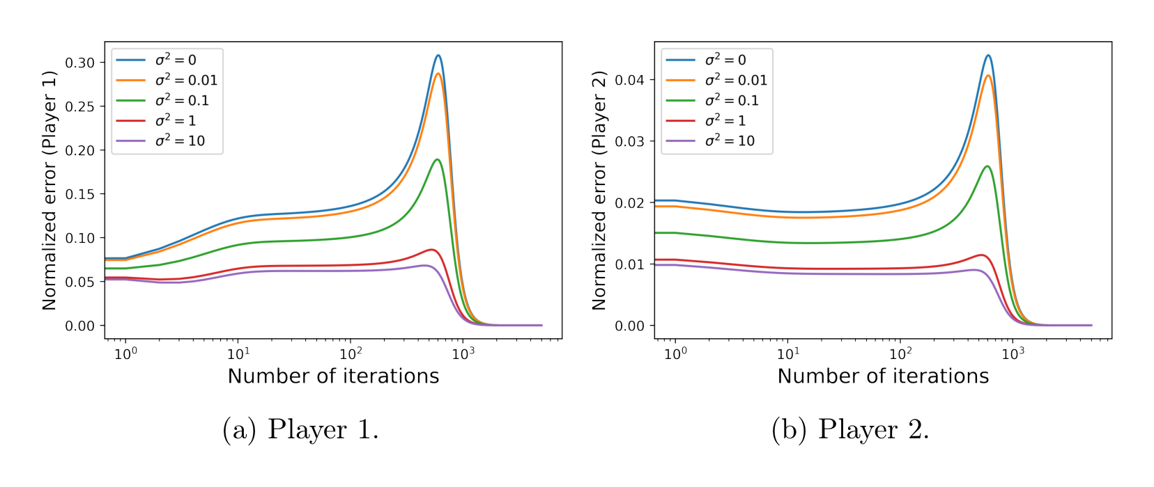
Convergence. The natural policy gradient algorithm shows a reasonable level of accuracy within 1000 iterations (that is, the normalized error is less than 0.5%) for both players under different levels of system noise σ2\sigma^2σ2, which ranges from 0 (deterministic dynamics) to 10. See Figure 1 for the case where r=0.25r=0.25r=0.25 and Figure 2 for the case where r=0.30r=0.30r=0.30. We observe that when we initialize the policies in a larger neighborhood of the Nash equilibrium, it takes the natural policy gradient algorithm (with the same step size) more iterations to converge. There is a sharp peak in the normalized error for player 2 and this peak diminishes when the noise level increases.
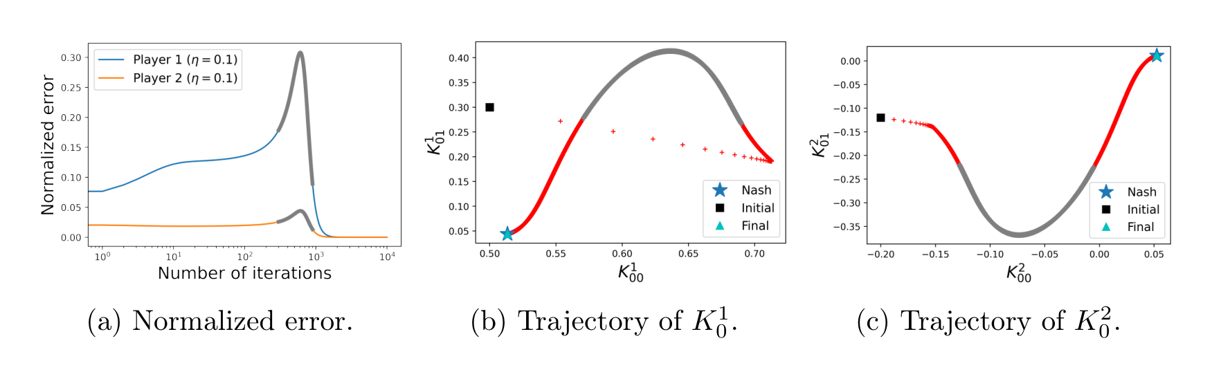
In Figure 3, we show the normalized error and the corresponding trajectories of learned policies near the peak observed in Figure 2 under σ=0\sigma=0σ=0. We denote by K0i=(K00i,K01i)K^i_0=(K^i_{00},K^i_{01})K0i=(K00i,K01i) the learned policy at t=0t=0t=0 of player iii. The peak period (iterations 300–900) is indicated in grey in Figures 3a–3c, and the trajectories of learned policy K0iK^i_0K0i for the rest of the whole 10000 iterations are indicated in red in Figures 3b–3c. The natural policy gradient algorithm overshoots in the first few iterations but detects the right direction after about 500 iterations and eventually converges to the Nash equilibrium (see the blue star in Figures 3b–3c).
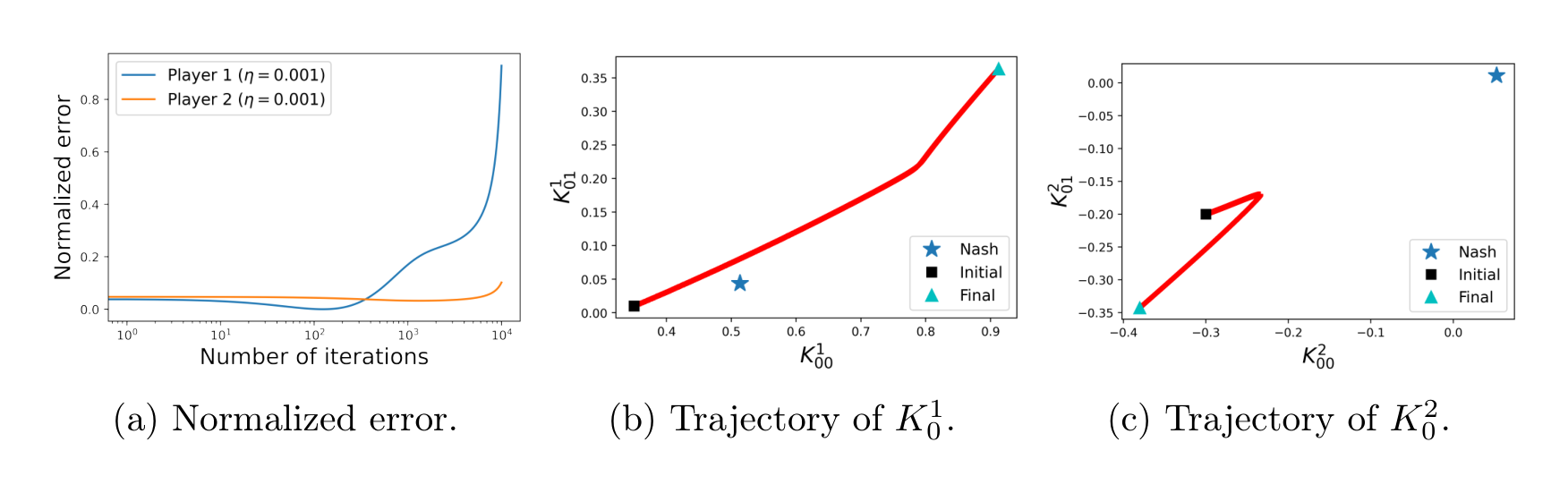
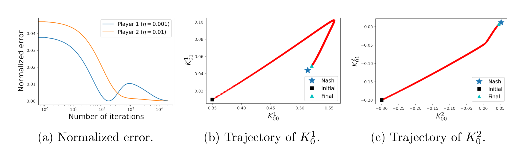
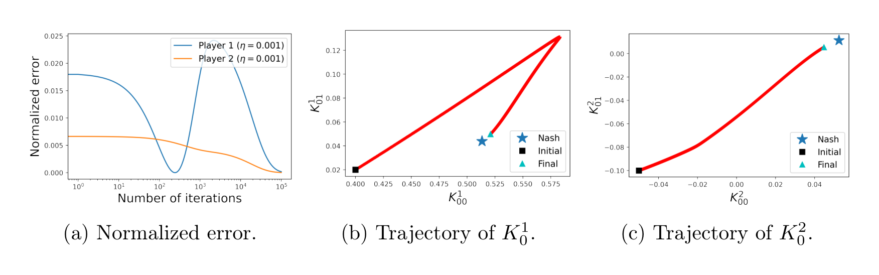
Performance under Deterministic Dynamics. We observe that under carefully chosen initial policies and step sizes, the natural policy gradient converges to the Nash equilibrium even with deterministic state dynamics (σ=0\sigma=0σ=0). We first show the case when the natural policy gradient algorithm diverges with r=0.42r=0.42r=0.42 and η1=η2=0.001\eta_1=\eta_2=0.001η1=η2=0.001 in Figure 4 (a trajectory of 10000 iterations is indicated in red). However, either by adjusting the step size to η2=0.01\eta_2=0.01η2=0.01 (see Figure 5), or by initializing the policies from a smaller neighbourhood around the Nash equilibrium (see Figure 6), the natural policy gradient method converges to the Nash equilibrium. This further demonstrates that the theoretical result, along with its assumptions, in Theorem 6 could provide insightful guidance on how to tune the hyper-parameters for practical examples.
5.2 Effect of the System Noise
As illustrated in the theoretical analysis in Section 3, the system noise plays an important role in the convergence guarantee of the natural policy gradient algorithm. To test the sensitivity of the performance of this algorithm to the level of system noise, we apply the natural policy gradient algorithm with unknown parameters to a two-player LQ game example with synthetic data consisting of a two-dimensional state variable and a one-dimensional control variable. The model parameters (except the level of noise σ2\sigma^2σ2 in WWW, which we will discuss later) are randomly picked such that the conditions for our LQ game framework are satisfied.
Set-up. We perform the natural policy gradient algorithm with synthetic data given as follows.
- Parameters: for t=1,…,T−1t=1,\ldots,T-1t=1,…,T−1,
where σ∈R+\sigma\in\mathbb{R}_+σ∈R+ and T=5T=5T=5. The smoothing parameter is r1=r2=0.5r_1=r_2=0.5r1=r2=0.5 and the number of trajectories is L1=L2=200L_1=L_2=200L1=L2=200.
- Initialization: we assume x0=(x01,x02)x_0=(x^1_0,x^2_0)x0=(x01,x02) with x01x^1_0x01 and x02x^2_0x02 independent and sampled from N(10,2)\mathcal{N}(10,2)N(10,2) and N(12,3)\mathcal{N}(12,3)N(12,3) respectively. The initial policy for player 1: K1∈R1×10=(K01,(0),…,KT−11,(0))K^1\in\mathbb{R}^{1\times 10}=(K^{1,(0)}_0,\ldots,K^{1,(0)}_{T-1})K1∈R1×10=(K01,(0),…,KT−11,(0)) with Kt1,(0)=[0.3,0.15]K^{1,(0)}_t=[0.3,0.15]Kt1,(0)=[0.3,0.15] for all ttt. The initial policy for player 2: K2∈R1×10=(K02,(0),…,KT−12,(0))K^2\in\mathbb{R}^{1\times 10}=(K^{2,(0)}_0,\ldots,K^{2,(0)}_{T-1})K2∈R1×10=(K02,(0),…,KT−12,(0)) with Kt2,(0)=[0.1,0.05]K^{2,(0)}_t=[0.1,0.05]Kt2,(0)=[0.1,0.05] for all ttt.
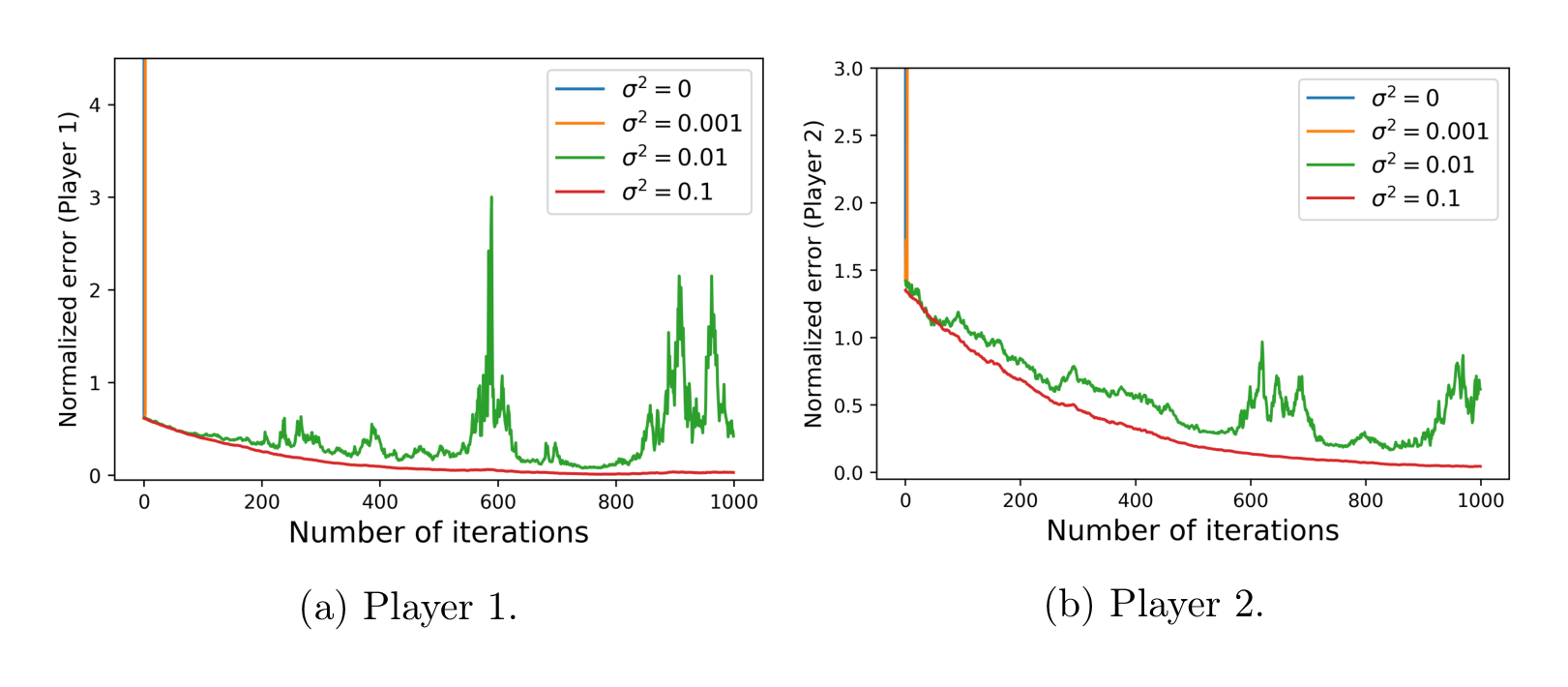
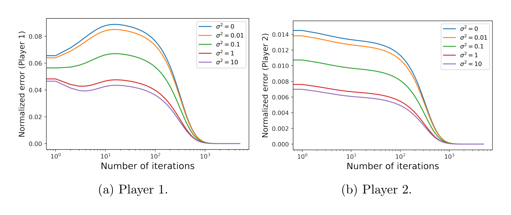
Convergence. To show that even a low level of system noise can indeed help the natural policy gradient algorithm to find the Nash equilibrium, we vary the value of σ2\sigma^2σ2 from 0 to 0.1 and show the normalized error for different values of σ2\sigma^2σ2 in Figure 7. The natural policy gradient algorithm diverges when σ2≤0.001\sigma^2\leq0.001σ2≤0.001 for both players, and it starts to converge with large fluctuations when σ2=0.01\sigma^2=0.01σ2=0.01. When σ2=0.1\sigma^2=0.1σ2=0.1, the algorithm shows a reasonable accuracy within 300 iterations (that is, the normalized error is less than 5%) for both players without fluctuations. It is worth pointing out that in fact, although Assumption 4 is violated when σ2=0.1\sigma^2=0.1σ2=0.1, the natural policy gradient algorithm converges to the Nash equilibrium. Finally, it is possible to make the algorithm converge when σ2≤0.001\sigma^2\leq0.001σ2≤0.001 by adjusting the initial policy and the step size, as shown in Section 5.1. In practice we may not be able to change the variance of wtw_twt directly, however the level of system noise can also be increased by adding (Gaussian) explorations to the agents’ policies. See Houthooft et al. (2016); Wang et al. (2020) for more discussion of Gaussian exploration.
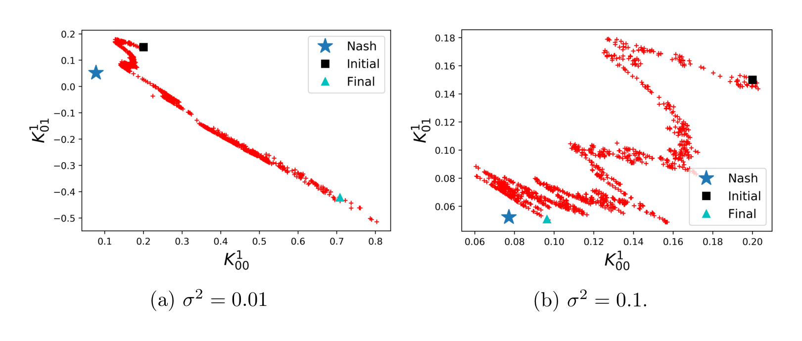
Trajectories of Learned Policies. We show the trajectories of the learned policy at t=0t=0t=0 of player 1 by performing the natural policy gradient algorithm with unknown parameters under σ2=0.01\sigma^2=0.01σ2=0.01 and σ2=0.1\sigma^2=0.1σ2=0.1 in Figure 8 (with 1000 iterations). In the case of a lower level of system noise (σ2=0.01\sigma^2=0.01σ2=0.01), the natural policy gradient does not converge to Nash equilibrium with η1=η2=0.001\eta_1=\eta_2=0.001η1=η2=0.001 in Figure 8a, whereas when the level of noise is increased to σ2=0.1\sigma^2=0.1σ2=0.1, the learned policy approaches the target within 1000 iterations with the same step size.
5.3 Convergence in a Three-player Game
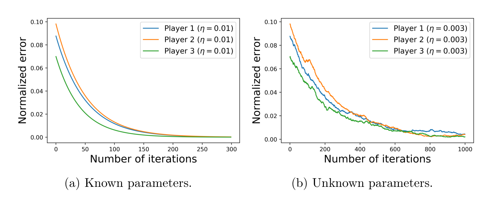
In this section, we perform the natural policy gradient method with known and unknown parameters in the following three-player general-sum game example. We show the convergence of the algorithms in Figure 9.
Set-up. We set up the model parameters and initial policies as follows.
- Parameters:
- Initialization: Take x0=(x01,x02,x03)x_0=(x^1_0,x^2_0,x^3_0)x0=(x01,x02,x03) where x01,x02,x03x^1_0,x^2_0,x^3_0x01,x02,x03 are independent and sampled from N(0.3,0.2)\mathcal{N}(0.3,0.2)N(0.3,0.2), N(0.2,0.3)\mathcal{N}(0.2,0.3)N(0.2,0.3), and N(0.3,0.2)\mathcal{N}(0.3,0.2)N(0.3,0.2) respectively. The initial policies are K1,(0)=(0.35,0.01,0.1)K^{1,(0)}=(0.35,0.01,0.1)K1,(0)=(0.35,0.01,0.1), K2,(0)=(−0.3,−0.2,0)K^{2,(0)}=(-0.3,-0.2,0)K2,(0)=(−0.3,−0.2,0), and K3,(0)=(−0.3,0.1,0)K^{3,(0)}=(-0.3,0.1,0)K3,(0)=(−0.3,0.1,0).
Convergence. We plot the normalized error for each player in the case of known parameters and also unknown parameters in Figure 9. We can see that with three players, the algorithms still have a reasonably fast speed of convergence in practice.
Acknowledgments
We thank Paul Barnes and Amr El Zanfally at bp plc for providing part of the motivation for this work and for their continued support. Huining Yang was supported by the EPSRC Centre for Doctoral Training in Industrially Focused Mathematical Modelling (EP/L015803/1) in collaboration with bp plc.
Appendix A. The One-step Contraction Lemma for the Vanilla Policy Gradient Method
The convergence result for the natural policy gradient method can be extended to the case of the vanilla policy gradient method. The key step is to prove the one-step contraction (Lemma 19) for the vanilla version. This can be done by modifying some parts of the current Lemma 19. We first recall the definition of g1g_1g1 and g2g_2g2 as follows:
and
We further define g~2\tilde{g}_2g~2 as
and g3g_3g3 as
We also write Ci,−i∗=Ci(Ki,K−i∗)C^{i,-i*}=C^i(K^i,K^{-i*})Ci,−i∗=Ci(Ki,K−i∗), Ci∗=Ci(K∗)C^{i*}=C^i(K^*)Ci∗=Ci(K∗) and Ci0,−i∗=Ci(Ki0,K−i∗)C^{i0,-i*}=C^i(K^{i0},K^{-i*})Ci0,−i∗=Ci(Ki0,K−i∗) to simplify notation.
Remark 1. We compare the noise condition (A.3) for the vanilla policy gradient method and the condition (3.56) for the natural version in Lemma 19. We mainly focus on the orders of NNN, TTT, and ρK\rho_KρK, and ignore other constants in (A.3) and (3.56). For the natural version, we need
For the vanilla version, we need
The order of ρK\rho_KρK is higher in (A.8), and the orders of TTT and (N−1)(N-1)(N−1) are slightly higher in (A.7). Thus when ρKT\rho_K^TρKT is small, the vanilla method has a weaker noise assumption. This may happen when the time horizon TTT is small and the policy KKK is close to the Nash equilibrium. In contrast, when ρKT\rho_K^TρKT is large, (A.7) is weaker than (A.8) and the natural method is superior to the vanilla method. Additionally, when N−1N-1N−1 is very large (and ρKT\rho_K^TρKT does not blow up), (A.8) leads to a weaker assumption.
We also note that other than the noise condition, there are also some slight differences between the step size conditions (A.5) for the vanilla method and (3.58) for the natural method, mainly in the order of ρK2T\rho_K^{2T}ρK2T appearing in the denominator of I1I_1I1, I3I_3I3, and I4I_4I4.
Proof [Proof of Lemma 1.] We break this proof up into a series of steps.
Step 1: We first consider the consequences of the condition η≤min{I3,I4}\eta\leq\min\{I_3,I_4\}η≤min{I3,I4}. Straightforward calculations show that when condition η≤I3\eta\leq I_3η≤I3 is satisfied, the following inequalities hold:
- For all i=1,…,Ni=1,\ldots,Ni=1,…,N,
- For all i=1,…,Ni=1,\ldots,Ni=1,…,N,
- For all i=1,…,Ni=1,\ldots,Ni=1,…,N,
In the case where η≤I4\eta\leq I_4η≤I4, we have, for all i=1,…,Ni=1,\ldots,Ni=1,…,N,
By (A.9) and Lemma 13 we have
Therefore, we have ρK,K′≤ρK\rho_{K,K'}\leq\rho_KρK,K′≤ρK by Lemma 15.
Steps 2 and 3: The results in Steps 2 and 3 in Lemma 19 for the natural policy gradient method still hold for the vanilla policy gradient method by the consequences (A.9) and (A.10). Here we omit the proof and state the following results which will be used in Steps 4 and 5:
Step 4: We can now estimate the cost difference between using KiK^iKi and the update Ki0K^{i0}Ki0. By Lemma 12 we have
For the vanilla policy gradient method, we have the following update rule:
by Lemma 9. Then plugging in Kti0−Kti=−2ηEt,iKΣtKK^{i0}_t-K^i_t=-2\eta E^K_{t,i}\Sigma^K_tKti0−Kti=−2ηEt,iKΣtK into (A.15) leads to
where the first equation holds by the updating rule, the second equation holds by adding and subtracting Et,iKi,K−i∗E^{K^i,K^{-i*}}_{t,i}Et,iKi,K−i∗ and Et,iKi,K−i∗ΣtKi0,K−i∗E^{K^i,K^{-i*}}_{t,i}\Sigma^{K^{i0},K^{-i*}}_tEt,iKi,K−i∗ΣtKi0,K−i∗ terms, and the third equation holds by expanding terms. Now, letting ω2=2/σX\omega^2=2/\sigma_Xω2=2/σX in
which holds for any matrices AAA and BBB of the same dimension, the second term in (A.16) can be bounded by
Now using the fact (A.17) again with ω2=2/σX2\omega^2=2/\sigma_X^2ω2=2/σX2, we can also bound the second last term in (A.16) as follows:
Then plugging the above bounds into (A.16) gives
where the first inequality holds by (A.18) and (A.19), and the second inequality holds by the trace inequality (3.33) and rearranging terms. Now we bound the term ∥ΣtK∥\|\Sigma^K_t\|∥ΣtK∥. By (3.39) and (3.49) we have
By (A.3) we have σX2≥g3\sigma_X^2\geq g_3σX2≥g3, which implies
Now, since ∥ΣKi0,K−i∗∥≤2Ci,−i∗/σQ\|\Sigma^{K^{i0},K^{-i*}}\|\leq2C^{i,-i*}/\sigma_Q∥ΣKi0,K−i∗∥≤2Ci,−i∗/σQ by (A.13), we can bound the step size condition in (A.11) by
Combining (A.22) and (A.23) gives
Hence, using this in (A.20), we have
where
Therefore, by (A.14), (A.13), Lemma 11, and Lemma 13,
where
Step 5: Finally we can establish the one step contraction. Using (A.26), we have
Hence by Lemma 12 and (3.42), we have
and thus
Summing up (A.29) for i=1,…,Ni=1,\ldots,Ni=1,…,N, we have
Since η≤I4\eta\leq I_4η≤I4, we have (A.12) and then
and hglob≤hˉglobh_{\mathrm{glob}}\leq\bar{h}_{\mathrm{glob}}hglob≤hˉglob, where hˉglob\bar{h}_{\mathrm{glob}}hˉglob is given by
Under condition (A.3), we have
which indicates that αη>0\alpha\eta>0αη>0. Since η≤∥ΣK∗∥σX2σR\eta\leq\frac{\|\Sigma_{K^*}\|}{\sigma_X^2\sigma_R}η≤σX2σR∥ΣK∗∥ by assumption, we have
Recall that in the statement we define α=σX2g1−g~2/σX5\alpha=\sigma_X^2g_1-\tilde{g}_2/\sigma_X^5α=σX2g1−g~2/σX5. Therefore we have αη<1\alpha\eta<1αη<1. Along with (A.30), we obtain the one-step contraction (A.6).
We now explain the main differences between the above proof and the proof for the natural policy gradient method. Since for the vanilla method we have Kti0−Kti=−2ηEt,iKΣtKK^{i0}_t-K^i_t=-2\eta E^K_{t,i}\Sigma^K_tKti0−Kti=−2ηEt,iKΣtK rather than Kti0−Kti=−2ηEt,iKK^{i0}_t-K^i_t=-2\eta E^K_{t,i}Kti0−Kti=−2ηEt,iK in the case of the natural version, the extra ΣtK\Sigma^K_tΣtK term needs to be dealt with when calculating the individual cost difference Ci0,−i∗−Ci,−i∗C^{i0,-i*}-C^{i,-i*}Ci0,−i∗−Ci,−i∗. More precisely, the presence of ΣtK\Sigma^K_tΣtK causes more terms which need to be bounded (see Equation A.18) when finding an upper bound on Ci0,−i∗−Ci,−i∗C^{i0,-i*}-C^{i,-i*}Ci0,−i∗−Ci,−i∗ in (A.16), and the term ∥ΣtK∥\|\Sigma^K_t\|∥ΣtK∥ also needs to be bounded above (see Equation A.21). Due to these extra terms, the amount of noise needed in the system has a more complex form given in (A.3), where a new g3g_3g3 is introduced to guarantee (A.24) holds. This further demonstrates that the natural policy gradient method can be considered as a normalized version of the vanilla policy gradient method.
References
James Drew Bagnell and Jeff Schneider. Covariant policy search. In Proceedings of 18th International Joint Conference on Artificial Intelligence, pages 1019–1024, August 2003.
David Balduzzi, Sebastien Racaniere, James Martens, Jakob Foerster, Karl Tuyls, and Thore Graepel. The mechanics of n-player differentiable games. In International Conference on Machine Learning, pages 354–363. PMLR, 2018.
Tamer Başar and Geert Jan Olsder. Dynamic Non-Cooperative Game Theory. Society for Industrial and Applied Mathematics, 1998.
Matteo Basei, Xin Guo, Anran Hu, and Yufei Zhang. Logarithmic regret for episodic continuous-time linear-quadratic reinforcement learning over a finite-time horizon. Journal of Machine Learning Research, 23(178):1–34, 2022.
Michael Bowling and Manuela Veloso. Multiagent learning using a variable learning rate. Artificial Intelligence, 136(2):215–250, 2002.
Jingjing Bu, Lillian Ratliff, and Mehran Mesbahi. Global convergence of policy gradient for sequential zero-sum linear quadratic dynamic games. arXiv preprint arXiv:1911.04672, 2019.
Maryam Fazel, Rong Ge, Sham Kakade, and Mehran Mesbahi. Global convergence of policy gradient methods for the linear quadratic regulator. In International Conference on Machine Learning, pages 1467–1476. PMLR, 2018.
Tanner Fiez, Benjamin Chasnov, and Lillian Ratliff. Implicit learning dynamics in Stackelberg games: Equilibria characterization, convergence analysis, and empirical study. In International Conference on Machine Learning, pages 3133–3144. PMLR, 2020.
Jakob Foerster, Richard Chen, Maruan Al-Shedivat, Shimon Whiteson, Pieter Abbeel, and Igor Mordatch. Learning with opponent-learning awareness. In Proceedings of the 17th International Conference on Autonomous Agents and MultiAgent Systems, pages 122–130, 2018.
Ian Gemp and Sridhar Mahadevan. Global convergence to the equilibrium of GANs using variational inequalities. arXiv preprint arXiv:1808.01531, 2018.
Ben Hambly, Renyuan Xu, and Huining Yang. Policy gradient methods for the noisy linear quadratic regulator over a finite horizon. SIAM Journal on Control and Optimization, 59(5):3359–3391, 2021.
Rein Houthooft, Xi Chen, Yan Duan, John Schulman, Filip De Turck, and Pieter Abbeel. VIME: Variational information maximizing exploration. Advances in neural information processing systems, 29, 2016.
Minyi Huang, Roland Malhamé, and Peter Caines. Large population stochastic dynamic games: Closed-loop McKean-Vlasov systems and the Nash certainty equivalence principle. Communications in Information and Systems, 6(3):221–252, 2006.
Junqi Jin, Chengru Song, Han Li, Kun Gai, Jun Wang, and Weinan Zhang. Real-time bidding with multi-agent reinforcement learning in display advertising. In Proceedings of the 27th ACM International Conference on Information and Knowledge Management, pages 2193–2201, 2018.
Sham Kakade. A natural policy gradient. Advances in Neural Information Processing Systems, 14, 2001.
Jean-Michel Lasry and Pierre-Louis Lions. Mean field games. Japanese Journal of Mathematics, 2(1):229–260, 2007.
Alistair Letcher, David Balduzzi, Sébastien Racaniere, James Martens, Jakob Foerster, Karl Tuyls, and Thore Graepel. Differentiable game mechanics. Journal of Machine Learning Research, 20(1):3032–3071, 2019.
Horia Mania, Stephen Tu, and Benjamin Recht. Certainty equivalence is efficient for linear quadratic control. In Advances in Neural Information Processing Systems, pages 10154–10164, 2019.
Eric Mazumdar, Lillian Ratliff, Michael Jordan, and Sosale Shankara Sastry. Policy-gradient algorithms have no guarantees of convergence in linear quadratic games. In Proceedings of the 19th International Conference on Autonomous Agents and MultiAgent Systems, pages 860–868, 2020a.
Eric Mazumdar, Lillian Ratliff, and Shankar Sastry. On gradient-based learning in continuous games. SIAM Journal on Mathematics of Data Science, 2(1):103–131, 2020b.
Panayotis Mertikopoulos, Christos Papadimitriou, and Georgios Piliouras. Cycles in adversarial regularized learning. In Proceedings of the Twenty-Ninth Annual ACM-SIAM Symposium on Discrete Algorithms, pages 2703–2717. SIAM, 2018.
Jorge Nocedal and Stephen Wright. Numerical optimization. Springer Science & Business Media, 2006.
Jan Peters and Stefan Schaal. Natural actor-critic. Neurocomputing, 71(7-9):1180–1190, 2008.
Aravind Rajeswaran, Kendall Lowrey, Emanuel Todorov, and Sham Kakade. Towards generalization and simplicity in continuous control. Advances in Neural Information Processing Systems, 30, 2017.
Masoud Roudneshin, Jalal Arabneydi, and Amir Aghdam. Reinforcement learning in nonzero-sum linear quadratic deep structured games: Global convergence of policy optimization. In 2020 59th IEEE Conference on Decision and Control, pages 512–517. IEEE, 2020.
Joan Saniuk and Ian Rhodes. A matrix inequality associated with bounds on solutions of algebraic Riccati and Lyapunov equations. IEEE Transactions on Automatic Control, 32(8):739–740, 1987. doi: 10.1109/TAC.1987.1104700.
John Schulman, Sergey Levine, Pieter Abbeel, Michael Jordan, and Philipp Moritz. Trust region policy optimization. In International Conference on Machine Learning, pages 1889–1897. PMLR, 2015.
Shai Shalev-Shwartz, Shaked Shammah, and Amnon Shashua. Safe, multi-agent, reinforcement learning for autonomous driving. arXiv preprint arXiv:1610.03295, 2016.
Satinder Singh, Michael Kearns, and Yishay Mansour. Nash convergence of gradient dynamics in general-sum games. In Proceedings of the Sixteenth conference on Uncertainty in Artificial Intelligence, pages 541–548, 2000.
Xinliang Song, Tonghan Wang, and Chongjie Zhang. Convergence of multi-agent learning with a finite step size in general-sum games. In Proceedings of the 18th International Conference on Autonomous Agents and MultiAgent Systems, pages 935–943, 2019.
Emmanouil-Vasileios Vlatakis-Gkaragkounis, Lampros Flokas, Thanasis Lianeas, Panayotis Mertikopoulos, and Georgios Piliouras. No-regret learning and mixed Nash equilibria: They do not mix. Advances in Neural Information Processing Systems, 33:1380–1391, 2020.
Haoran Wang, Thaleia Zariphopoulou, and Xun Yu Zhou. Reinforcement learning in continuous time and space: A stochastic control approach. Journal of Machine Learning Research, 21:198–1, 2020.
Sheng-De Wang, Te-Son Kuo, and Chen-Fa Hsu. Trace bounds on the solution of the algebraic matrix Riccati and Lyapunov equation. IEEE Transactions on Automatic Control, 31(7):654–656, 1986.
Chongjie Zhang and Victor Lesser. Multi-agent learning with policy prediction. In Twenty-fourth AAAI conference on artificial intelligence, 2010.
Junzi Zhang, Jongho Kim, Brendan O’Donoghue, and Stephen Boyd. Sample efficient reinforcement learning with REINFORCE. In Proceedings of the AAAI Conference on Artificial Intelligence, volume 35, pages 10887–10895, 2021a.
Kaiqing Zhang, Zhuoran Yang, and Tamer Başar. Policy optimization provably converges to Nash equilibria in zero-sum linear quadratic games. In Advances in Neural Information Processing Systems, 2019.
Kaiqing Zhang, Xiangyuan Zhang, Bin Hu, and Tamer Başar. Derivative-free policy optimization for linear risk-sensitive and robust control design: Implicit regularization and sample complexity. Advances in Neural Information Processing Systems, 34:2949–2964, 2021b.