Rectified Linear Units Improve Restricted Boltzmann Machines

Vinod Nair [email protected]
Geoffrey E. Hinton [email protected]
Department of Computer Science, University of Toronto, Toronto, ON M5S 2G4, Canada

Abstract

Restricted Boltzmann machines were developed using binary stochastic hidden units. These can be generalized by replacing each binary unit by an infinite number of copies that all have the same weights but have progressively more negative biases. The learning and inference rules for these “Stepped Sigmoid Units” are unchanged. They can be approximated efficiently by noisy, rectified linear units. Compared with binary units, these units learn features that are better for object recognition on the NORB dataset and face verification on the Labeled Faces in the Wild dataset. Unlike binary units, rectified linear units preserve information about relative intensities as information travels through multiple layers of feature detectors.

Executive Summary: The paper examines how to improve restricted Boltzmann machines (RBMs), a type of generative model used to learn features from data such as images. Binary hidden units, the standard approach, limit the amount of information that can pass through each layer and lose relative intensity details. This matters because RBMs are often stacked into deeper networks for tasks like object recognition, where preserving intensity relationships and achieving good performance on complex natural scenes are critical.

The work set out to test whether replacing binary hidden units with noisy rectified linear units (NReLUs) would produce stronger features for downstream recognition. The authors first show that an infinite collection of binary units with offset biases closely approximates a rectified linear function and that a simple noisy version of this function can be sampled efficiently. They then compare the two unit types on two standard vision benchmarks.

Both models were trained on the same data using contrastive divergence for pre-training, followed by supervised fine-tuning. Experiments used the Jittered-Cluttered NORB dataset (roughly 292,000 training images of toys under varied pose and lighting) and the Labeled Faces in the Wild dataset (over 13,000 face images evaluated in 10-fold cross-validation). Single- and two-layer architectures were tested, with hidden-layer sizes up to 4,000 units; images were downsampled to 32\times32 pixels and normalized before training.

NReLUs consistently outperformed binary units. On NORB, two-layer NReLU models reached 15.2 % test error with full pre-training, versus 18.8 % for binary units. On LFW, NReLUs achieved 80.7 % verification accuracy after pre-training, compared with 77.8 % for binary units. NReLUs without any pre-training still beat pre-trained binary models on NORB. In addition, zero-bias rectified units keep relative intensity information intact through multiple layers, enabling a simple cosine-distance classifier to become analytically invariant to positive intensity scaling—an effect binary units cannot provide.

These results indicate that the change of hidden-unit type improves both recognition accuracy and the model’s ability to represent intensity variations without extra parameters or architectural changes. Performance gains hold across random initialization and pre-training regimes, suggesting the advantage is not limited to one training regime.

Practitioners building RBM-based feature hierarchies for vision should adopt rectified linear units in place of binary units. When possible, pre-train at least the first hidden layer; adding a second pre-trained layer yields further gains with NReLUs. The approach can be combined with existing enhancements such as better face alignment or attribute labels.

The experiments used heavily downsampled images and only two datasets; variance on LFW is still sizable. Results should be confirmed on higher-resolution data and additional tasks before large-scale deployment.

1. Introduction

Section Summary: Restricted Boltzmann machines act as versatile generative models that can capture patterns in many kinds of data, from images and speech to documents and movie ratings, and they serve as building blocks for constructing deeper networks. The section explains a straightforward training procedure called contrastive divergence that tunes the connections between visible data units and hidden feature detectors by comparing correlations in real training examples with those in reconstructed versions. It also describes how the basic binary model can be adapted for continuous data by replacing visible units with Gaussian ones, often after normalizing the inputs to simplify learning.

Restricted Boltzmann machines (RBMs) have been used as generative models of many different types of data including labeled or unlabeled images (Hinton et al., 2006), sequences of mel-cepstral coefficients that represent speech (Mohamed & Hinton, 2010), bags of words that represent documents (Salakhutdinov & Hinton, 2009), and user ratings of movies (Salakhutdinov et al., 2007). In their conditional form they can be used to model high-dimensional temporal sequences such as video or motion capture data (Taylor et al., 2006). Their most important use is as learning modules that are composed to form deep belief nets (Hinton et al., 2006).

1.1. Learning a Restricted Boltzmann Machine

Images composed of binary pixels can be modeled by an RBM that uses a layer of binary hidden units (feature detectors) to model the higher-order correlations between pixels. If there are no direct interactions between the hidden units and no direct interactions between the visible units that represent the pixels, there is a simple and efficient method called “Contrastive Divergence” to learn a good set of feature detectors from a set of training images (Hinton, 2002). We start with small, random weights on the symmetric connections between each pixel $i$ and each feature detector $j$. Then we repeatedly update each weight, $w_{ij}$, using the difference between two measured, pairwise correlations

$ \Delta w_{ij} = \epsilon (\langle v_i h_j \rangle_{\text{data}} - \langle v_i h_j \rangle_{\text{recon}})\tag{1} $

where $\epsilon$ is a learning rate, $\langle v_i h_j \rangle_{\text{data}}$ is the frequency with which visible unit $i$ and hidden unit $j$ are on together when the feature detectors are being driven by images from the training set and $\langle v_i h_j \rangle_{\text{recon}}$ is the corresponding frequency when the hidden units are being driven by reconstructed images. A similar learning rule can be used for the biases.

Given a training image, we set the binary state, $h_j$, of each feature detector to be 1 with probability

$ p(h_j = 1) = \frac{1}{1 + \exp\left(-b_j - \sum_{i \in \text{vis}} v_i w_{ij}\right)}\tag{2} $

where $b_j$ is the bias of $j$ and $v_i$ is the binary state of pixel $i$. Once binary states have been chosen for the hidden units we produce a “reconstruction” of the training image by setting the state of each pixel to be 1 with probability

$ p(v_i = 1) = \frac{1}{1 + \exp\left(-b_i - \sum_{j \in \text{hid}} h_j w_{ij}\right)}\tag{3} $

The learned weights and biases implicitly define a probability distribution over all possible binary images via the energy, $E(\mathbf{v}, \mathbf{h})$, of a joint configuration of the visible and hidden units:

$ E(\mathbf{v}, \mathbf{h}) = -\sum_{i,j} v_i h_j w_{ij} - \sum_i v_i b_i - \sum_j h_j b_j\tag{4} $

$ p(\mathbf{v}) = \frac{\sum_{\mathbf{h}} e^{-E(\mathbf{v}, \mathbf{h})}}{\sum_{\mathbf{u}, \mathbf{g}} e^{-E(\mathbf{u}, \mathbf{g})}}\tag{5} $

1.2. Gaussian units

RBMs were originally developed using binary stochastic units for both the visible and hidden layers (Hinton, 2002). To deal with real-valued data such as the pixel intensities in natural images, (Hinton & Salakhutdinov, 2006) replaced the binary visible units by linear units with independent Gaussian noise as first suggested by (Freund & Haussler, 1994). The energy function then becomes:

$ E(\mathbf{v}, \mathbf{h}) = \sum_{i \in \text{vis}} \frac{(v_i - b_i)^2}{2\sigma_i^2} - \sum_{j \in \text{hid}} b_j h_j - \sum_{i,j} \frac{v_i}{\sigma_i} h_j w_{ij}\tag{6} $

where $\sigma_i$ is the standard deviation of the Gaussian noise for visible unit $i$.

It is possible to learn the variance of the noise for each visible unit but this is difficult using binary hidden units. In many applications, it is much easier to first normalise each component of the data to have zero mean and unit variance and then to use noise-free reconstructions, with the variance in equation 6 set to 1. The reconstructed value of a Gaussian visible unit is then equal to its top-down input from the binary hidden units plus its bias. We use this type of noise-free visible unit for the models of object and face images described later.

2. Rectified linear units

Section Summary: Researchers have shown that rectified linear units can be constructed by combining many binary units that share the same weights but have fixed, staggered biases. The combined activity of these units closely follows a smooth curve given by log(1 + e^x), producing an integer-valued, noisy version of a rectified linear response without adding extra learned parameters. A practical approximation replaces exact sampling with max(0, x plus Gaussian noise), yielding noisy rectified linear units that train more stably and perform better than ordinary binary hidden units on several tasks.

To allow each unit to express more information, (Teh & Hinton, 2001) introduced binomial units which can be viewed as $N$ separate copies of a binary unit that all share the same bias and weights. A nice side-effect of using weight-sharing to synthesize a new type of unit out of binary units is that the mathematics underlying learning in binary-binary RBM’s remains unchanged. Since all $N$ copies receive the same total input, they all have the same probability, $p$, of turning on and this only has to be computed once. The expected number that are on is $N p$ and the variance in this number is $N p(1-p)$. For small $p$, this acts like a Poisson unit, but as $p$ approaches 1 the variance becomes small again which may not be desireable. Also, for small values of $p$ the growth in $p$ is exponential in the total input. This makes learning much less stable than for the stepped sigmoid units (SSU) described next.

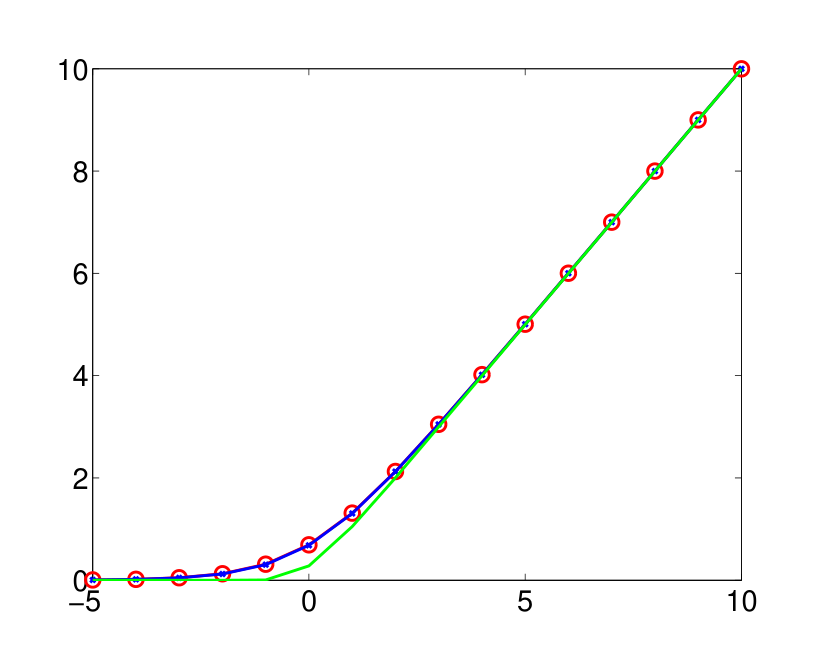
A small modification to binomial units makes them far more interesting as models of real neurons and also more useful for practical applications. We make an infinite number of copies that all have the same learned weight vector $\mathbf{w}$ and the same learned bias, $b$, but each copy has a different, fixed offset to the bias. If the offsets are $-0.5, -1.5, -2.5, \dots$ the sum of the probabilities of the copies is extremely close to having a closed form (figure 1):

$ \sum_{i=1}^N \sigma(x - i + 0.5) \approx \log(1 + e^x),\tag{7} $

where $x = \mathbf{v}\mathbf{w}^\top + b$.

So the total activity of all of the copies behaves like a noisy, integer-valued version of a smoothed rectified linear unit[^1]. Even though $\log(1 + e^x)$ is not in the exponential family, we can model it accurately using a set of binary units with shared weights and fixed bias offsets. This set has no more parameters than an ordinary binary unit, but it provides a much more expressive variable. The variance in the integer activity level is $\sigma(x)$ so units that are firmly off do not create noise and the noise does not become large when $x$ is large.

[^1]: If we only use $N$ copies, we need to subtract the term $\log(1 + e^{x-N})$ from the approximation.

A drawback of giving each copy a bias that differs by a fixed offset is that the logistic sigmoid function needs to be used many times to get the probabilities required for sampling an integer value correctly. It is possible, however, to use a fast approximation in which the sampled value of the rectified linear unit is not constrained to be an integer. Instead it is given by $\max(0, x + N(0, \sigma(x)))$ where $N(0, V)$ is Gaussian noise with zero mean and variance $V$. We call a unit that uses this approximation a Noisy Rectified Linear Unit (NReLU) and this paper shows that NReLUs work better than binary hidden units for several different tasks.

(Jarrett et al., 2009) have explored various rectified nonlinearities (including the $\max(0, x)$ nonlinearity, which they refer to as “positive part”) in the context of convolutional networks and have found them to improve discriminative performance. Our empirical results in sections 5 and 6 further support this observation. We also give an approximate probabilistic interpretation for the $\max(0, x)$ nonlinearity, further justifying their use.

3. Intensity equivariance

Section Summary: Rectified linear units with zero bias exhibit intensity equivariance, meaning that uniformly scaling all pixel intensities in an image by a positive factor causes the active units to scale their outputs by exactly the same factor while inactive units stay off. This property persists through successive layers of such units, unlike binary hidden units. The resulting feature vectors can therefore be compared with a cosine measure that remains unchanged under intensity shifts, providing a form of invariance better suited to recognition than simple pixel normalization.

NReLU’s have some interesting mathematical properties (Hahnloser et al., 2003), one of which is very useful for object recognition. A major consideration when designing an object recognition system is how to make the output invariant to properties of the input such as location, scale, orientation, lighting etc. Convolutional neural networks are often said to achieve translation invariance but in their pure form they actually achieve something quite different. If an object is translated in the input image, its representation in a pool of local filters that have shared weights is also translated. So if it can be represented well by a pattern of feature activities when it is in one location, it can also be represented equally well by a translated pattern of feature activities when it is another location. We call this translation equivariance: the representation varies in the same way as the image. In a deep convolutional net, translation invaraince is achieved by using subsampling to introduce a small amount of translation invariance after each layer of filters.

Binary hidden units do not exhibit intensity equivariance, but rectified linear units do, provided they have zero biases and are noise-free. Scaling up all of the intensities in an image by $\alpha > 0$ cannot change whether a zero-bias unit receives a total input above or below zero. So all of the “off” units remain off and the remainder all increase their activities by a factor of $\alpha$. This stays true for many layers of rectified linear units. When deciding whether two face images come from the same person, we make use of this nice property of rectified linear units by basing the decision on the cosine of the angle between the activities of the feature detectors in the last hidden layer. The feature vectors are intensity equivariant and the cosine is intensity invariant. The type of intensity invariance that is important for recognition cannot be achieved by simply dividing all the pixel intensities by their sum. This would cause a big change in the activities of feature detectors that attend to the parts of a face when there is a bright spot in the background.

4. Empirical Evaluation

Section Summary: Researchers tested a new type of neural network unit called NReLU against standard binary units on two difficult image tasks: recognizing objects in cluttered scenes and verifying whether two faces belong to the same person. They first trained the networks without labels to discover useful features, then adjusted them with labeled data, and found that the NReLU versions performed better on both tasks. For the final adjustment step they used a simple rule that outputs zero for negative inputs and the input value itself for positive ones, along with a matching gradient for learning.

We empirically compare NReLUs to stochastic binary hidden units[^2] on two vision tasks: 1) object recognition on the Jittered-Cluttered NORB dataset (LeCun et al., 2004), and 2) face verification on the Labeled Faces in the Wild dataset (Huang et al., 2007). Both datasets contain complicated image variability that make them difficult tasks. Also, they both already have a number of published results for various methods, which gives a convenient basis for judging how good our results are. We use RBMs with binary hidden units or NReLUs to generatively pre-train one or more layers of features and we then discriminatively fine-tune the features using backpropagation. On both tasks NReLUs give better discriminative performance than binary units. The discriminative models use the deterministic version of NReLUs that implement the function $y = \max(0, x)$. For backpropagation, we take the gradient of this function to be 0 when $x \le 0$ and 1 when $x > 0$ (i.e. we ignore the discontinuity at $x = 0$).

[^2]: We also compared with binomial units but they were no better than binary units, so we omit those results.

5. Jittered-Cluttered NORB

Section Summary: The Jittered-Cluttered NORB dataset contains stereo images of five toy classes (humans, animals, cars, planes, trucks) plus a no-object class, with random jitter, background clutter, and a peripheral distractor; training and test sets use entirely different object instances to test generalization. The authors subsample the images to 32x32 resolution, normalize them, and train classifiers by first pre-training two layers of restricted Boltzmann machines with either rectified linear or binary hidden units, then fine-tuning the full network via multinomial regression on the top layer. Results indicate that rectified linear units outperform binary ones both with and without pre-training, reaching a test error of 16.5 percent in the best configuration.

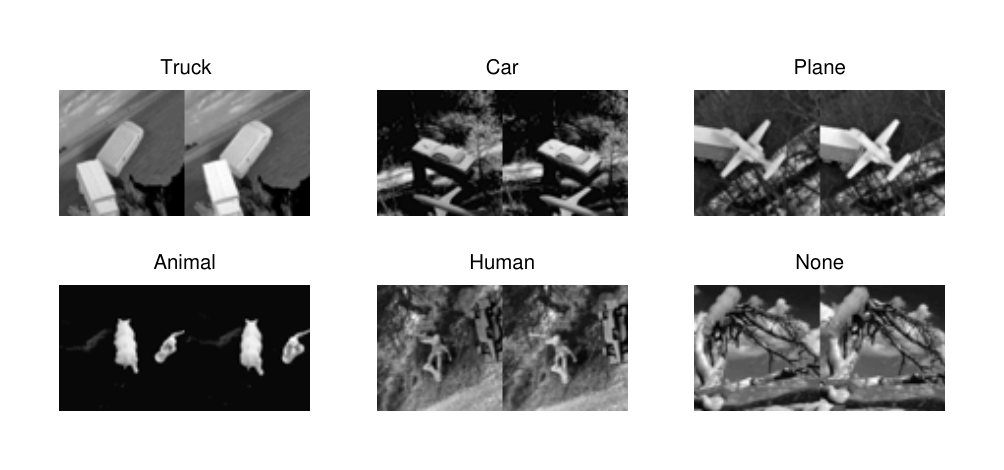
NORB is a synthetic 3D object recognition dataset that contains five classes of toys (humans, animals, cars, planes, trucks) imaged by a stereo-pair camera system from different viewpoints under different lighting conditions. NORB comes in several versions – the Jittered-Cluttered version has grayscale stereo-pair images with cluttered background and a central object which is randomly jittered in position, size, pixel intensity etc. There is also a distractor object placed in the periphery. Examples from the dataset are shown in figure 2. For each class, there are ten different instances, five of which are in the training set and the rest in the test set. So at test time a classifier needs to recognize unseen instances of the same classes. In addition to the five object classes, there is a sixth class whose images contain none of the objects in the centre. For details see (LeCun et al., 2004).

5.1. Training

The stereo-pair images are subsampled from their original resolution of $108 \times 108 \times 2$ to $32 \times 32 \times 2$ to speed up experiments. They are normalized to be zero-mean and divided by the average standard deviation of all the pixels in all the training images. There are 291,600 training cases (48,600 cases per class) and 58,320 test cases (9,720 cases per class). We hold out 58,320 cases from the training set and use them as a validation set for selecting the model architecture (number of hidden units and number of layers) and for early stopping. The validation set is created by taking all 9,720 training images of a single (randomly selected) object instance from each of the five object classes, and an equal number of randomly selected images from the “None” class.

To train a classifier we use a similar approach to (Larochelle et al., 2007). We first greedily pre-train two layers of features, each as an RBM using CD. Then we use multinomial regression at the top-most hidden layer to predict the label and discriminatively fine-tune the parameters in all layers of the classifier (see figure 3). We have tried 1000, 2000 and 4000 units for the first hidden layer, and 1000 and 2000 units for the second one. Using more units always gave better classification results, so the architecture with the best results have 4000 units in the first layer and 2000 in the second. We suspect that the results will be even better with more hidden units. In all cases, the pixels are represented by Gaussian units (Hinton & Salakhutdinov, 2006) and the hidden units are either NReLUs or stochastic binary units. Pre-training is done for 300 epochs (in both layers), using mini-batches of 100 training examples with a learning rate of $10^{-3}$ applied to the average per-case CD update, along with momentum (Hinton et al., 2006).

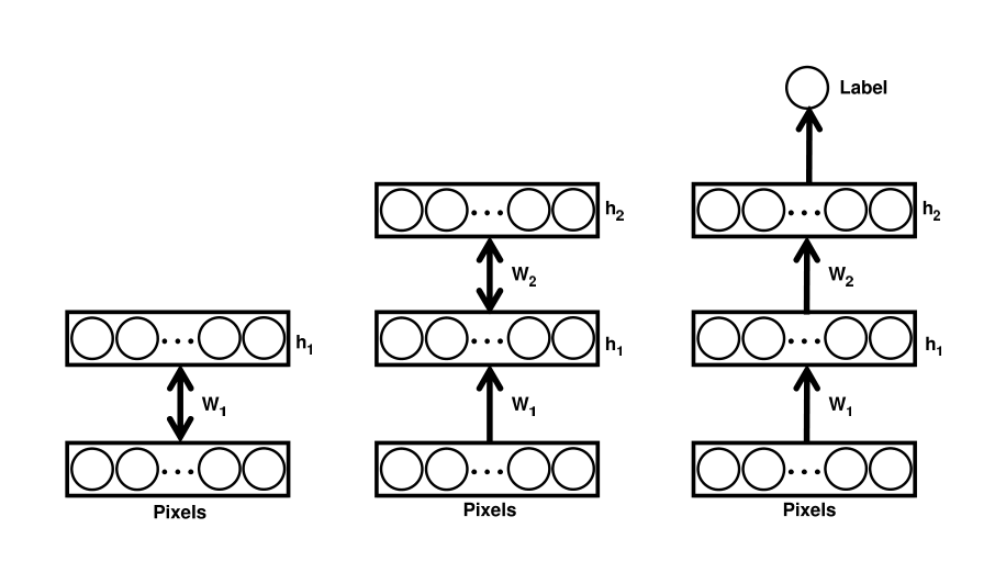
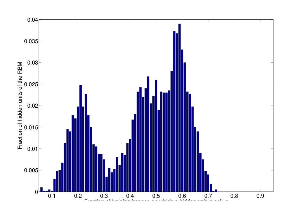
Figure 4 shows a subset of features learned by the first-level RBM with 4000 NReLUs in the hidden layer. Many of these are Gabor-like filters, so NReLUs seem capable of learning qualitatively sensible features from images. The classification results (section 5.2) show that they are quantitatively sensible as well. Figure 5 is a histogram that shows how often the hidden units in this RBM have values above zero on the training set. If a unit is always “active”, then it would end up in the rightmost bin of the histogram. Note that an always-active unit is purely linear since it never gets rectified. As the histgroam shows, there are no such units in this model. There is some variety in how often the units are active. We have looked at the features that correspond to each of the three peaks in the histogram: the peak near 0.2 on the x-axis are Gabor-like filters, while the peak near 0.6 are point filters. The smaller peak between 0.4 and 0.5 corresponds mostly to more global filters.

5.2. Classification Results

Table 1 lists the test set error rates of classifiers with a single hidden layer, using either binary units or NReLUs, with and without pre-training. NReLUs outperform binary units, both when randomly initialized and when pre-trained. Pre-training helps improve the performance of both unit types. But NReLUs without pre-training are better than binary units with pre-training.

: Table 1: Test error rates for classifiers with 4000 hidden units trained on $32 \times 32 \times 2$ Jittered-Cluttered NORB images.

\begin{tabular}{|c|c|c|}
\hline
\textbf{Pre-trained?} & \textbf{NReLU} & \textbf{Binary} \\
\hline
No & 17.8\% & 23.0\% \\
Yes & 16.5\% & 18.7\% \\
\hline
\end{tabular}

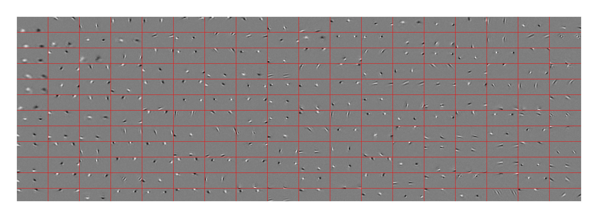
Table 2 lists the results for classifiers with two hidden layers. Just as for single hidden layer classifiers, NReLUs outperform binary units regardless of whether greedy pre-training is used only in the first layer, in both layers, or not at all. Pre-training improves the results: pre-training only the first layer and randomly initializing the second layer is better than randomly initialized both. Pre-training both layers gives further improvement for NReLUs but not for binary units.

: Table 2: Test error rates for classifiers with two hidden layers (4000 units in the first, 2000 in the second), trained on $32 \times 32 \times 2$ Jittered-Cluttered NORB images.

\begin{tabular}{|c|c|c|c|}
\hline
\textbf{Layer 1 pre-trained?} & \textbf{Layer 2 pre-trained?} & \textbf{NReLU} & \textbf{Binary} \\
\hline
No & No & 17.6\% & 23.6\% \\
Yes & No & 16.5\% & 18.8\% \\
Yes & Yes & 15.2\% & 18.8\% \\
\hline
\end{tabular}

For comparison, the error rates of some other models are: multinomial regression on pixels 49.9%, Gaussian kernel SVM 43.3%, convolutional net 7.2%, convolutional net with an SVM at the top-most hidden layer 5.9%. The last three results are from (Bengio & LeCun, 2007). Our results are worse than that of convolutional nets, but 1) our models use heavily subsampled images, and 2) convolutional nets have knowledge of image topology and approximate translation invariance hard-wired into their architecture.

6. Labeled Faces in the Wild

Section Summary: The Labeled Faces in the Wild dataset tests whether two face photos show the same person or different people. The approach uses a siamese neural network that processes each face separately with a shared feature extractor pretrained as a restricted Boltzmann machine, then combines the results with a symmetric cosine-distance measure to decide if the identities match. Images are tightly cropped and normalized around the face before training and testing on pairs whose identities never overlap between the training and evaluation sets.

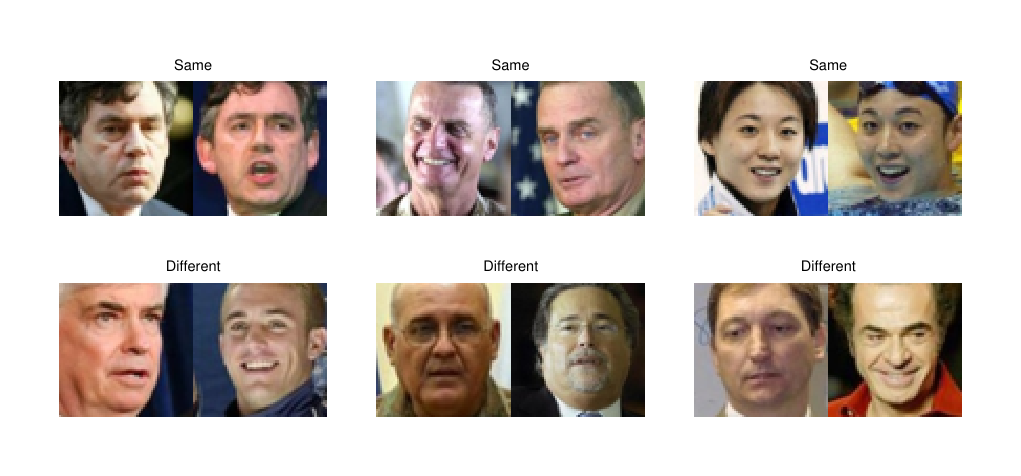
The prediction task for the Labeled Faces in the Wild (LFW) dataset is as follows: given two face images as input, predict whether the identities of the faces are the same or different. The dataset contains colour faces of public figures collected from the web using a frontal-face detector. The bounding box computed by the face detector is used to approximately normalize the face’s position and scale within the image. Some examples from the dataset are shown in figure 6. For details see (Huang et al., 2007).

6.1. Network architecture

The task requires a binary classifier with two sets of inputs (the two faces). If we stitch the two inputs together and treat the result as one extended input vector, the classifier’s output will depend on the order in which the inputs are stitched. To make the classifier symmetric with respect to the inputs, we use a siamese architecture (Chopra et al., 2005). The idea is to learn a function that takes a single face as input and computes some feature vector from it. Given a pair of faces, this function is applied to both faces separately, and the two corresponding feature vectors are combined using a fixed, symmetric function into a single representation which is invariant to input order. The probability of the two faces being the same person is computed as output from this representation. The entire system, including the feature extractor replicated over the two faces, can be learned jointly.

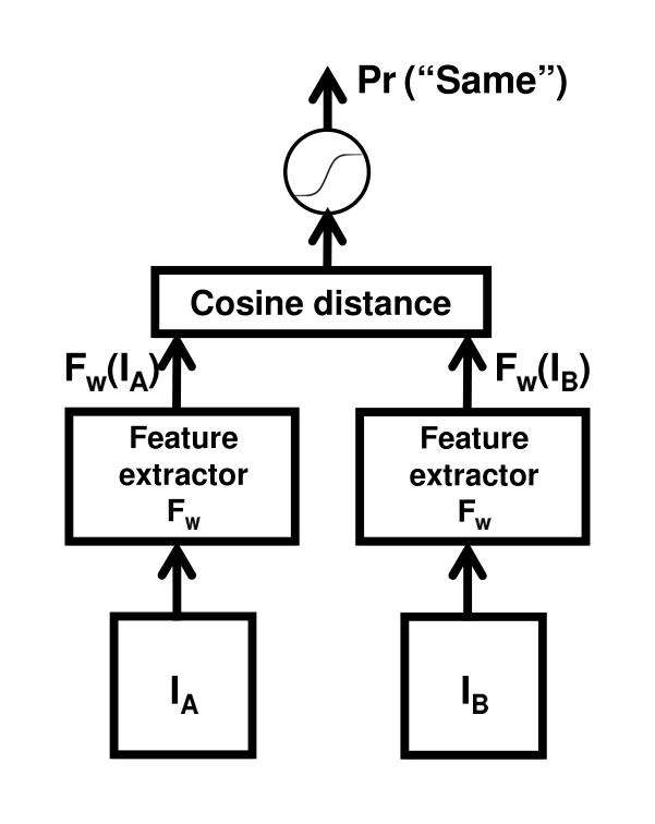
Here we choose the feature extractor to be a fully-connected feedforward layer of NReLUs, pre-trained as an RBM. We use cosine distance as the symmetric function that combines the two feature vectors. Cosine distance is invariant to rescaling of its inputs, which when combined with the equivariance of NReLUs makes the entire model analytically invariant to rescaling of the pixels by a positive scalar. The invariance holds regardless of the number of layers of NReLUs, so it is possible to train deep architectures with this property. In order to make the feature extractor exactly equivariant, we do not use biases into the hidden units. Figure 7 shows the architecture of our face verification model.

6.2. Training

LFW images are of size $250 \times 250$ ($\times 3$ colour channels) with the face in the centre and a lot of background surrounding it. Recently it has been found that humans are able to get 94.27% accuracy on the LFW task even when the centre of the image is masked (Kumar et al., 2009). To prevent background information from artificially inflating the results, we only use a $144 \times 144$ window from the centre. The images are then rotated and scaled such that the coordinates of the eyes are the same across all images. We further subsample this window to $32 \times 32$ ($\times 3$ channels). The same image normalization procedure used for Jittered-Cluttered NORB is applied here as well.

LFW contains 13,233 images of 5,749 people. For the purposes of reporting results, the designers of LFW have pre-defined 10 splits of the dataset for 10-fold cross validation, each containing 5,400 training pairs and 600 test pairs. The number of “same” and ”different” cases are always equal, both for training and test sets. The identities of the people in the training and test sets are always kept disjoint, so at test time the model must predict on unseen identities. We first pre-train a layer of features as an RBM using all 10,800 single faces in the training set of each split, then plug it into the siamese architecture in figure 7 and discriminatively fine-tune the parameters on pairs of faces. As before, during pre-training pixels are Gaussian units, and the hidden units are either NReLUs or stochastic binary units.

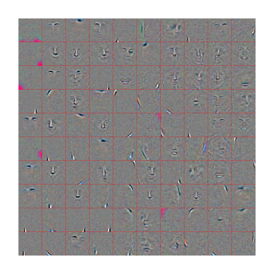
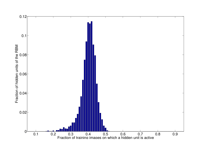
Figure 8 shows 100 of the 4000 features learned by an RBM on $32 \times 32$ colour images with NReLUs in the hidden layer. Like the NORB model in section 5.1, this model is also pre-trained for 300 epochs on mini-batches of size 100 with a learning rate of $10^{-3}$ and momentum. The model has learned detectors for parts of faces like eyes, nose, mouth, eye brows etc. Some features detect the boundary of the face. There is a mix of localized filters and more global ones that detect more than just a single part of the face. The histogram in figure 9 shows how often the units in this RBM turn on for the faces in LFW. Unlike the NORB model, here the histogram has only one peak. In particular, there are almost no point filters in this model.

During discriminative fine-tuning, we use a subset of the Pubfig face dataset (Kumar et al., 2009) as a validation set for selecting the model architecture and for early stopping. This subset, called the “development set” by the creators of Pubfig, do not contain any identities that are in LFW.

6.3. Classification Results

As explained before, after pre-training a single layer of features as an RBM, we insert it into the siamese architecture in figure 7 and discriminatively fine-tune the parameters. We have tried models with 1000, 2000, 4000 and 8000 units in the hidden layer. The difference in accuracy is small between 4000 and 8000 units – all the results in this section are for 4000 units.

The rules of LFW specify that a model’s accuracy must be computed using ten-fold cross validation using the ten pre-specified splits of the dataset. To speed up experiments, we merge two splits into one and perform five-fold cross validation. Table 3 lists the average accuracy of various models, along with the standard deviations. Models using NReLUs seem to be more accurate, but the standard deviations are too large to draw firm conclusions.

: Table 3: Accuracy on the LFW task for various models trained on $32 \times 32$ colour images.

\begin{tabular}{|c|c|c|}
\hline
\textbf{Pre-trained?} & \textbf{NReLU} & \textbf{Binary} \\
\hline
No & 0.7925 $\pm$ 0.0173 & 0.7768 $\pm$ 0.0070 \\
Yes & 0.8073 $\pm$ 0.0134 & 0.7777 $\pm$ 0.0109 \\
\hline
\end{tabular}

The two current best LFW results are $0.8683 \pm 0.0034$ (Wolf et al., 2009), and $0.8529 \pm 0.0123$ (Kumar et al., 2009). The former uses a commercial automatic face alignment system to normalize the faces, while the latter uses additional labels (collected manually) that describe the face, such as ethnicity, sex, age etc. Such enhancements can be applied to our model as well, and they are likely to increase accuracy significantly. These results may also be benefiting from the background pixels around the face, which we have (mostly) removed here.

7. Mixtures of Exponentially Many Linear Models

Section Summary: Rectified linear units offer an efficient way to model the density of complex, high-dimensional data that has componential structure, such as images containing multiple independent elements. Instead of needing an exponentially large number of mixture components, as in standard approaches like mixtures of Gaussians, a modest number of these units can implicitly define a different linear model in each of 2^N regions on a hypersphere while sharing parameters across all of them. This approach also avoids the inference difficulties and density discontinuities that arise in earlier directed models of exponentially many linear mixtures.

We have shown that NReLUs work well for discrimination, but they are also an interesting way of modeling the density of real-valued, high-dimensional data. A standard way to do this is to use a mixture of diagonal Gaussians. Alternatively we can use a mixture of factor analysers. Both of these models are exponentially inefficient if the data contains componential structure. Consider, for example, images of pairs of independent digits. If a mixture model for single digit images needs $N$ components, a single mixture model of pairs of digits needs $N^2$ components. Fortunately, this exponential growth in the number of components in the mixture can be achieved with only linear growth in the number of latent variables and quadratic growth in the number of parameters if we use rectified linear hidden units.

Consider using rectified linear units with zero bias to model data that lies on the surface of a unit hypersphere. Each rectified linear unit corresponds to a plane through the centre of the hypersphere. It has an activity of 0 for one half of the hypersphere and for the other half its activity increases linearly with distance from that plane. $N$ units can create $2^N$ regions on the surface of the hypersphere[^3]. As we move around within each of these regions the subset of units that are non-zero does not change so we have a linear model, but it is a different linear model in every region. The mixing proportions of the exponentially many linear models are defined implicitly by the same parameters as are used to define $p(\mathbf{v}|\mathbf{h})$ and, unlike a directed model, the mixing proportions are hard to compute explicitly (Nair & Hinton, 2008).

[^3]: Assuming the hypersphere is at least $N$-dimensional.

This is a much better way of implementing an exponentially large mixture of linear models with shared latent variables than the method described in (Hinton et al., 1999) which uses directed linear models as the components of the mixture and a separate sigmoid belief net to decide which hidden units should be part of the current linear model. In that model, it is hard to infer the values of the binary latent variables and there can be jumps in density at the boundary between two linear regions. A big advantage of switching between linear models at the point where a hidden unit receives an input of exactly zero is that it avoids discontinuities in the modeled probability density.

8. Summary

Section Summary: Researchers developed a more powerful type of hidden unit for restricted Boltzmann machines by linking the weights and biases of an infinite collection of simpler binary units, then approximating the result with noisy rectified linear units. These units outperformed standard binary hidden units on tasks such as object recognition and face comparison, and they handled wide variations in input intensity more naturally. The approach also lets the model represent mixtures of many linear patterns using only a modest number of parameters.

We showed how to create a more powerful type of hidden unit for an RBM by tying the weights and biases of an infinite set of binary units. We then approximated these stepped sigmoid units with noisy rectified linear units and showed that they work better than binary hidden units for recognizing objects and comparing faces. We also showed that they can deal with large intensity variations much more naturally than binary units. Finally we showed that they implement mixtures of undirected linear models (Marks & Movellan, 2001) with a huge number of components using a modest number of parameters.

References

Section Summary: This section compiles a bibliography of scholarly papers and technical reports that underpin research in artificial intelligence and machine learning. The cited works emphasize neural networks, unsupervised learning methods, and practical uses such as face verification and object recognition, with frequent contributions from researchers like Geoffrey Hinton, Yann LeCun, and Yoshua Bengio. Overall, the list reflects foundational studies from the 1990s through the late 2000s that advanced techniques for handling complex data patterns.

Bengio, Y. and LeCun, Y. Scaling learning algorithms towards AI. 2007.

Chopra, S., Hadsell, R., and LeCun, Y. Learning a similarity metric discriminatively, with application to face verification. In CVPR, pp. 539–546, Washington, DC, USA, 2005. IEEE Computer Society.

Freund, Y. and Haussler, D. Unsupervised learning of distributions on binary vectors using two layer networks. Technical report, Santa Cruz, CA, USA, 1994.

Hahnloser, Richard H. R., Seung, H. Sebastian, and Slotine, Jean-Jacques. Permitted and forbidden sets in symmetric threshold-linear networks. Neural Computation, 15(3):621–638, 2003. ISSN 0899-7667.

Hinton, G. E. Training products of experts by minimizing contrastive divergence. Neural Computation, 14(8):1711–1800, 2002.

Hinton, G. E. and Salakhutdinov, R. Reducing the dimensionality of data with neural networks. Science, 313:504–507, 2006.

Hinton, G. E., Sallans, B., and Ghahramani, Z. A hierarchical community of experts. pp. 479–494, 1999.

Hinton, G. E., Osindero, S., and Teh, Y. A fast learning algorithm for deep belief nets. Neural Computation, 18:1527–1554, 2006.

Huang, G. B., Ramesh, M., Berg, T., and Learned-Miller, E. Labeled Faces in the Wild: A Database for Studying Face Recognition in Unconstrained Environments. Technical Report 07-49, University of Massachusetts, Amherst, 2007.

Jarrett, K., Kavukcuoglu, K., Ranzato, M., and LeCun, Y. What is the best multi-stage architecture for object recognition? In Proc. International Conference on Computer Vision (ICCV’09). IEEE, 2009.

Kumar, N., Berg, A. C., Belhumeur, P. N., and Nayar, S. K. Attribute and simile classifiers for face verification. In International Conference on Computer Vision, 2009.

Larochelle, H., Erhan, D., Courville, A., Bergstra, J., and Bengio., Y. An empirical evaluation of deep architectures on problems with many factors of variation. In ICML, pp. 473–480, 2007.

LeCun, Y., Huang, F. J., and Bottou., L. Learning methods for generic object recognition with invariance to pose and lighting. In CVPR, Washington, D.C., 2004.

Marks, T. K. and Movellan, J. R. Diffusion networks, products of experts, and factor analysis. Technical Report UCSD MPLab TR 2001.02, 2001.

Mohamed, A. and Hinton, G. E. Phone recognition using restricted boltzmann machines. In ICASSP, Dallas, TX, USA, 2010.

Nair, V. and Hinton, G. E. Implicit mixtures of restricted boltzmann machines. In Neural information processing systems, 2008.

Salakhutdinov, R. and Hinton, G. E. Replicated softmax: an undirected topic model. In Advances in Neural Information Processing Systems 22, 2009.

Salakhutdinov, R., Mnih, A., and Hinton, G. E. Restricted Boltzmann machines for collaborative filtering. In Proceedings of the International Conference on Machine Learning, volume 24, pp. 791–798, 2007.

Taylor, G. W., Hinton, G. E., and Roweis, S. Modeling human motion using binary latent variables. In Advances in Neural Information Processing Systems 19, Cambridge, MA, 2006. MIT Press.

Teh, Y.W. and Hinton, G. E. Rate-coded restricted boltzmann machines for face recognition. In Advances in Neural Information Processing Systems, volume 13, 2001.

Wolf, L., Hassner, T., and Taigman, Y. Similarity scores based on background samples. In Asian Conference on Computer Vision, 2009.