Diffeomorphic Optimization

Ludwig WinklerAndrew Leaver-FayJoseph KleinhenzPan Kessel

article2026arXiv0 citations

Introduces diffeomorphic optimization to perform Riemannian gradient descent through the base space of generative models, extending the framework to Lie groups to achieve superior accuracy and speed in computational protein design.

Listen

Computational design of complex biological structures, such as therapeutic proteins and peptide binders, relies heavily on generative artificial intelligence models to propose physically valid molecular geometries. While these models excel at learning the underlying distribution of realistic biological structures, steering them to optimize specific functional goals—such as binding affinity, physical stability, or custom secondary structures—remains difficult. Traditional optimization techniques that directly adjust atomic coordinates in physical space frequently produce deformed, non-viable molecules because the underlying physical energy landscapes are rugged, highly non-convex, and prone to severe local traps.

The article demonstrates a novel optimization framework called diffeomorphic optimization, which optimizes differentiable objective functions on the data manifold by performing gradient descent within the simpler, smooth latent base space of pretrained generative diffusion and flow models. The study evaluates this approach across several challenging structural biology tasks, including protein backbone reshaping, small-molecule docking, peptide design, and atomic-level energy minimization.

The approach leverages the smooth, invertible mapping learned by flow and diffusion models to translate simple latent coordinates into valid three-dimensional molecular structures. The authors provide mathematical proofs showing that stepping through this latent space is equivalent to performing Riemannian gradient descent on the data manifold, guaranteeing that generated molecules stay physically plausible throughout the process. To handle complex geometric transformations involving three-dimensional rotations and translations in protein backbones, the authors introduced Lie-group integration tools compatible with standard automatic differentiation software, as well as an adjoint-state differential equation solver.

The investigation produced three central findings. First, on protein secondary structure targeting using the FrameFlow model, diffeomorphic optimization placed 91.3% of residues into the desired structural region, substantially outperforming heavily tuned guidance baselines that reached only 63.3%. Second, on peptide binder design, the method generated higher stability and binding affinity than previous optimal control approaches while running at twice the execution speed. Third, when paired with AlphaFlow and evaluated across hundreds of test proteins, the method reduced Rosetta physical energy scores by thousands of units compared to the industry-standard Rosetta Relax protocol, achieving superior energetic minima that could not be matched by standard relaxation even when baseline computing budgets were substantially increased.

These results indicate that generative models can serve as smooth, constraint-preserving search spaces for molecular engineering without requiring model retraining, reward fine-tuning, or complex auxiliary networks. By replacing inefficient brute-force sampling and filtering with targeted gradient-based refinement, the methodology can substantially improve candidate quality before initiating expensive and time-consuming laboratory wet-lab experiments.

Organizations developing computational molecular design pipelines should evaluate diffeomorphic optimization as an inference-time refinement layer for existing generative workflows that use differentiable scoring functions. For practical software implementations, teams should adopt autograd-compatible checkpointing methods, which exhibited greater numerical stability than adjoint-state methods when integrating through stiff ordinary differential equations.

The primary operational limitation is the heightened computational cost per generated design due to iterative backpropagation through numerical differential equation solvers. However, empirical ablations demonstrate that the optimization remains robust even when using coarse solver schedules with as few as 10 to 25 steps, providing a flexible trade-off between computational overhead and optimization fidelity.

arXiv: 2607.00947

No sufficiently relevant recommendations were found.
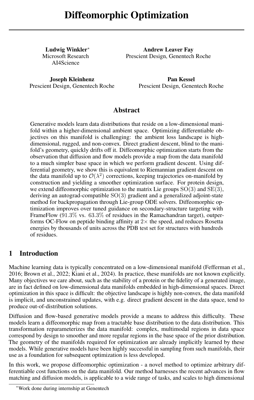
Cover for Diffeomorphic Optimization

Abstract

Generative models learn data distributions that reside on a low-dimensional manifold within a higher-dimensional ambient space. Optimizing differentiable objectives on this manifold is challenging: the ambient loss landscape is high-dimensional, rugged, and non-convex. Direct gradient descent, blind to the manifold's geometry, quickly drifts off it. Diffeomorphic optimization starts from the observation that diffusion and flow models provide a map from the data manifold to a much simpler base space in which we perform gradient descent. Using differential geometry, we show this is equivalent to Riemannian gradient descent on the data manifold up to O(λ2)\mathcal{O}(\lambda^2) corrections, keeping trajectories on-manifold by construction and yielding a smoother optimization surface. For protein design, we extend diffeomorphic optimization to the matrix Lie groups SO(3)\mathrm{SO}(3) and SE(3)\mathrm{SE}(3), deriving an autograd-compatible SO(3)\mathrm{SO}(3) gradient and a generalized adjoint-state method for backpropagation through Lie-group ODE solvers. Diffeomorphic optimization improves over tuned guidance on secondary-structure targeting with FrameFlow (91.3%91.3\% vs. 63.3%63.3\% of residues in the Ramachandran target), outperforms OC-Flow on peptide binding affinity at 2×2\times the speed, and reduces Rosetta energies by thousands of units across the PDB test set for structures with hundreds of residues.

Table of Contents

  • 1 Introduction
  • 2 Related Works
  • 3 Diffeomorphic Optimization stays on Manifold
  • 3.1 Basics Concepts of Differential Geometry
  • 3.2 Diffeomorphic optimization is equivalent to Gradient Descent on the Data Manifold
  • 4 Backpropagation through 𝐒𝐄⁡(𝟑)\mathbf{SE(3)} ODE solvers
  • 4.1 Gradients of 𝐒𝐄⁡(𝟑)\mathbf{SE(3)} Solvers
  • 5 Experiments
  • 6 Conclusion and Limitations
  • References
  • A Riemannian Gradient Implementation for 𝐒𝐎⁡(𝟑)\mathbf{SO(3)}
  • B Expanded Related Work
  • C Proofs
  • C.1 Proof of Theorem
  • C.2 Proof of Theorem
  • C.3 Proof of Theorem
  • D Lightning Review of Differential Geometry and Lie Groups
  • E SO(3) Conventions
  • F Limitations of Guidance
  • G Complexity and Efficiency of Gradient Estimations through Flows
  • H Experiments
  • H.1 SO(3) Manifolds
  • H.2 Secondary Structure Optimization
  • H.3 Docking Optimization
  • H.4 Tertiary Structure Optimization

Knowls

  1. Knowl 1 — Diffeomorphic Optimization on Learned Data Manifolds

    model/method

    Generative diffusion and continuous normalizing flow models learn a smooth, invertible (diffeomorphic) map g:Z→D⊂Xg: \mathcal{Z} \to \mathcal{D} \subset \mathcal{X} from a tractable base space Z\mathcal{Z} (equipped with a standard unimodal distribution such as N(0,I)\mathcal{N}(0, I)) to a low-dimensional data manifold D\mathcal{D} embedded in an ambient space X\mathcal{X}. The forward mapping is defined by integrating the ordinary differential equation (ODE):

    g(z)≡x1=z+∫01vθ(xτ,τ) dτg(z) \equiv x_1 = z + \int_0^1 v_\theta(x_\tau, \tau) \, d\tau

    where τ∈[0,1]\tau \in [0, 1] is the integration time, vθv_\theta is a parameterized neural vector field, and x0=z∈Zx_0 = z \in \mathcal{Z}.

    Given an arbitrary differentiable cost function L:X→R\mathcal{L}: \mathcal{X} \to \mathbb{R} (such as protein stability or molecular docking energy), diffeomorphic optimization optimizes the loss directly on the manifold by reparameterizing in the base space variables as L(g(z))\mathcal{L}(g(z)) and executing gradient descent in Z\mathcal{Z} with learning rate λ∈R\lambda \in \mathbb{R}:

    z(i+1)=z(i)−λ∇zL(g(z(i)))z^{(i+1)} = z^{(i)} - \lambda \nabla_z \mathcal{L}(g(z^{(i)}))

    for iterations i∈{0,…,n−1}i \in \{0, \dots, n-1\}, subsequently evaluating the final data-space sample as x(n)=g(z(n))x^{(n)} = g(z^{(n)}). Because gg is a diffeomorphism onto D\mathcal{D}, the trajectory remains on the learned data manifold by construction, avoiding off-manifold drift while leveraging the regularized, unimodal geometry of Z\mathcal{Z} for improved mode-switching.

  2. Knowl 2 — Equivalence of Latent Gradient Descent to Riemannian Gradient Descent on the Data Manifold

    theoretical result

    Let g:Z→Dg: \mathcal{Z} \to \mathcal{D} be a diffeomorphic generative model mapping latent space Z\mathcal{Z} to the data manifold D\mathcal{D}, and let L:D→R\mathcal{L}: \mathcal{D} \to \mathbb{R} be a differentiable loss function. Let G~\tilde{G} be a Riemannian metric on Z\mathcal{Z}, and let G=g∗G~G = g_* \tilde{G} denote the pushforward metric on D\mathcal{D}, defined by G(u,v)=G~(dg−1u,dg−1v)G(u, v) = \tilde{G}(dg^{-1}u, dg^{-1}v) for tangent vectors u,v∈Tg(z)Du, v \in T_{g(z)}\mathcal{D}.

    Up to quadratic corrections in the learning rate λ∈R\lambda \in \mathbb{R}, performing gradient descent in the latent space Z\mathcal{Z} and projecting to D\mathcal{D} via gg is equivalent to Riemannian gradient descent directly on the data manifold D\mathcal{D}:

    g(exp⁡z(−λgrad⁡zG~(L∘g)))=exp⁡g(z)(−λgrad⁡g(z)GL+O(λ2))g\left(\exp_z\left(-\lambda \operatorname{grad}_z^{\tilde{G}} (\mathcal{L} \circ g)\right)\right) = \exp_{g(z)}\left(-\lambda \operatorname{grad}_{g(z)}^G \mathcal{L} + \mathcal{O}(\lambda^2)\right)

    where exp⁡p\exp_p denotes the Riemannian exponential map at point pp, and grad⁡G\operatorname{grad}^G denotes the Riemannian gradient.

    In local coordinates, the data-space gradient is given by:

    grad⁡g(z)L=Jggrad⁡zL,where Jg=∂g∂z\operatorname{grad}_{g(z)} \mathcal{L} = J_g \operatorname{grad}_z \mathcal{L}, \quad \text{where } J_g = \frac{\partial g}{\partial z}

    Under singular value decomposition (SVD) of the Jacobian JgJ_g, the effective learning rate along directions with low singular values is suppressed, aligning the gradient updates with the implicitly learned tangent space spanned by the dominant left-singular vectors.

  3. Knowl 3 — Decoupled Riemannian Gradient Descent on SE(3)

    model/method

    In rigid-body macromolecular modeling, each protein residue backbone frame is represented as an element T=(R,t)∈SE(3)=SO(3)⋉R3T = (R, t) \in SE(3) = SO(3) \ltimes \mathbb{R}^3, with rotation matrix R∈SO(3)R \in SO(3) and translation vector t∈R3t \in \mathbb{R}^3. Under the right-invariant Riemannian metric on SE(3)SE(3) defined as the direct sum of the Riemannian metrics on SO(3)SO(3) (induced by the Killing form) and Euclidean R3\mathbb{R}^3, the exponential maps and Riemannian gradients decouple:

    exp⁡T(ω,v)=(exp⁡R(ω),exp⁡t(v)),grad⁡TL=(grad⁡RL,grad⁡tL)\exp_T(\omega, v) = (\exp_R(\omega), \exp_t(v)), \quad \operatorname{grad}_T \mathcal{L} = (\operatorname{grad}_R \mathcal{L}, \operatorname{grad}_t \mathcal{L})

    for Lie algebra rotation vector ω∈so(3)\omega \in \mathfrak{so}(3), translational vector v∈R3v \in \mathbb{R}^3, and loss L:SE(3)→R\mathcal{L}: SE(3) \to \mathbb{R}.

    Consequently, the Riemannian gradient descent update at step ii with learning rate λ∈R\lambda \in \mathbb{R} decouples into standard vector translation and Lie-group exponential rotation:

    t(i+1)=t(i)−λ∇tL(R(i),t(i))t^{(i+1)} = t^{(i)} - \lambda \nabla_t \mathcal{L}(R^{(i)}, t^{(i)})

    R(i+1)=exp⁡(−λ∇RL(R(i),t(i)))R(i)R^{(i+1)} = \exp\left(-\lambda \nabla_R \mathcal{L}(R^{(i)}, t^{(i)})\right) R^{(i)}

    where exp⁡(A)=∑k=0∞Akk!\exp(A) = \sum_{k=0}^\infty \frac{A^k}{k!} is the matrix exponential, and ∇RL∈so(3)\nabla_R \mathcal{L} \in \mathfrak{so}(3) is the Lie algebra representative of the Riemannian gradient.

  4. Knowl 4 — Autograd Formulation for SO(3) Riemannian Gradients

    theoretical result

    Let L:SO(3)→R\mathcal{L}: SO(3) \to \mathbb{R} be a differentiable loss function on the 3D rotation group SO(3)SO(3), and let dLdR∈R3×3\frac{d\mathcal{L}}{dR} \in \mathbb{R}^{3 \times 3} denote the standard matrix-calculus ambient gradient with respect to the rotation matrix R∈SO(3)R \in SO(3). The Lie algebra representative ∇L(R)∈so(3)\nabla \mathcal{L}(R) \in \mathfrak{so}(3) of the Riemannian gradient is given by:

    ∇L(R)=2[dLdRR⊤]A\nabla \mathcal{L}(R) = 2 \left[ \frac{d\mathcal{L}}{dR} R^\top \right]_A

    where [M]A=12(M−M⊤)[M]_A = \frac{1}{2}(M - M^\top) denotes the antisymmetric projection of a 3×33 \times 3 matrix MM.

    This closed form allows standard automatic differentiation engines (such as PyTorch autograd) to compute exact Riemannian gradients on SO(3)SO(3): wrapping an SO(3)SO(3)-valued leaf tensor with a backward hook that computes GR⊤−(GR⊤)⊤G R^\top - (G R^\top)^\top (where G=dLdRG = \frac{d\mathcal{L}}{dR} is the incoming gradient) transforms Euclidean backpropagation into Riemannian gradient computation without dedicated Lie-group autograd backends.

  5. Knowl 5 — Generalized Adjoint-State Method for Lie-Group ODE Solvers

    theoretical result

    Consider a continuous-time generative flow ODE initial value problem on SE(3)SE(3):

    dTτ=(dZτ,dzτ)=(Vθ(Zτ,zτ),vθ(Zτ,zτ)) dτ,T0=(Z0,z0)=(Z,z)d T_\tau = (d Z_\tau, d z_\tau) = (V_\theta(Z_\tau, z_\tau), v_\theta(Z_\tau, z_\tau)) \, d\tau, \quad T_0 = (Z_0, z_0) = (Z, z)

    where τ∈[0,1]\tau \in [0, 1], Zτ∈SO(3)Z_\tau \in SO(3), zτ∈R3z_\tau \in \mathbb{R}^3, Vθ∈so(3)V_\theta \in \mathfrak{so}(3), and vθ∈R3v_\theta \in \mathbb{R}^3. Let (R,t)=g(Z,z)≡(Z1,z1)(R, t) = g(Z, z) \equiv (Z_1, z_1) and let L:SE(3)→R\mathcal{L}: SE(3) \to \mathbb{R} be a loss function.

    The Riemannian gradient with respect to the initial rotation condition Z∈SO(3)Z \in SO(3) is obtained as ∇ZL(g(Z,z))=A0\nabla_Z \mathcal{L}(g(Z, z)) = A_0, where the Lie-algebra-valued adjoint state Aτ=∑i=13AτiTi∈so(3)A_\tau = \sum_{i=1}^3 A_\tau^i T^i \in \mathfrak{so}(3) is solved backwards in time via the terminal value problem:

    dAτdτ=[Vθ(Zτ,zτ),Aτ]−∑i=13Aτi∇ZτVθi(Zτ,zτ),A1=∇RL(R,t)\frac{d A_\tau}{d\tau} = [V_\theta(Z_\tau, z_\tau), A_\tau] - \sum_{i=1}^3 A_\tau^i \nabla_{Z_\tau} V_\theta^i(Z_\tau, z_\tau), \quad A_1 = \nabla_R \mathcal{L}(R, t)

    where [A,B]=AB−BA[A, B] = AB - BA is the matrix commutator and {Ti}i=13\{T^i\}_{i=1}^3 are the orthonormal generators of so(3)\mathfrak{so}(3).

    For the translational component z∈R3z \in \mathbb{R}^3, the gradient is dL(g(Z,z))dz=a0\frac{d\mathcal{L}(g(Z, z))}{dz} = a_0, where the adjoint state aτ∈R3a_\tau \in \mathbb{R}^3 satisfies:

    daτdτ=−∑i=13aτidvθi(Zτ,zτ)dzτ,a1=dL(R,t)dt\frac{d a_\tau}{d\tau} = -\sum_{i=1}^3 a_\tau^i \frac{d v_\theta^i(Z_\tau, z_\tau)}{d z_\tau}, \quad a_1 = \frac{d\mathcal{L}(R, t)}{dt}

    This formulation applies to any matrix Lie group and avoids storing intermediate forward activations, achieving O(L)O(L) memory complexity.

  6. Knowl 6 — Peptide Design Performance Comparison Between Diffeomorphic Optimization and OC-Flow

    data/table

    The table evaluates diffeomorphic optimization (DiffeoOpt) against the PepFlow baseline and optimal control flow matching variants (OC-Flow controlling translations, rotations, or both) from Wang et al. (2024) across seven peptide design metrics: MadraX score (lower is better), backbone RMSD (Å, lower is better), secondary structure recovery percentage (SSR %, higher is better), backbone structure recovery percentage (BSR %, higher is better), stability energy (lower is better), binding affinity energy (lower is better), and structural diversity (higher is better). DiffeoOpt optimizes both translational and rotational base variables using repurposed autograd, outperforming all OC-Flow variants on MadraX (-0.309), BSR % (0.881), stability (-49.417), affinity (-28.409), and diversity (0.340) while maintaining low RMSD (1.605 Å) and running at 2×2\times the speed of OC-Flow.

    Method MadraX ↓\downarrow RMSD ↓\downarrow SSR % ↑\uparrow BSR % ↑\uparrow Stability ↓\downarrow Affinity ↓\downarrow Diversity ↑\uparrow
    Ground-truth -0.588 – – – -84.893 -36.063 –
    PepFlow -0.195 1.645 0.794 0.874 -45.660 -26.538 0.310
    OC-Flow(trans) -0.229 1.774 0.797 0.876 -48.380 -27.328 0.323
    OC-Flow(rot) -0.221 1.643 0.794 0.872 -48.636 -27.211 0.310
    OC-Flow(trans+rot) -0.263 2.127 0.797 0.869 -48.853 -27.468 0.338
    DiffeoOpt -0.309 1.605 0.796 0.881 -49.417 -28.409 0.340
  7. Knowl 7 — Secondary Structure Modification with FrameFlow Outperforms Diffusion Guidance

    empirical result

    Diffeomorphic optimization was evaluated on secondary structure redesign using FrameFlow, an SE(3)SE(3) backbone flow-matching model, by targeting dihedral angles in the Ramachandran map under the ABEGO scheme. Starting from structures predominantly in the α\alpha-helical (A) region, the objective minimized a modified Ramachandran/p_aa_pp energy term in tmol to drive residue dihedral angles towards the target β\beta-sheet (B) region.

    Across 50 generated protein structures, diffeomorphic optimization (using 25 Euler integration steps and 500 gradient steps in the base space with learning rate 0.1) shifted residues into the target A classification at 91.3±8.4%91.3 \pm 8.4\% (with 7.4±7.3%7.4 \pm 7.3\% in B), compared to the unguided baseline of 53.5±23.3%53.5 \pm 23.3\% in A (32.8±20.1%32.8 \pm 20.1\% in B).

    Guidance baselines with varying sampling steps (200, 500, 1000) and multi-step denoising allocations (1 to 200 denoiser steps per ODE step) peaked at 65.3±23.1%65.3 \pm 23.1\% in target residue classification. Diffeomorphic optimization achieved significantly higher targeting efficiency with substantially reduced variance across samples, while preserving designability.

  8. Knowl 8 — Optimization of Protein-Ligand Docking Scores Using DiffDock Base Space

    empirical result

    Diffeomorphic optimization was applied to DiffDock, an SE(3)×SO(2)kSE(3) \times SO(2)^k diffusion model for molecular docking, converted into a deterministic probability flow ODE to enable differentiable generation. The objective maximized the Vina docking score via OpenDock (a differentiable PyTorch implementation of AutoDock Vina) across approximately 78 PDBBind test set complexes with initial DiffDock confidence logits >0> 0.

    Base-space optimization was executed using 10 Adam steps (base learning rate 0.1, with rotation and torsion learning rates scaled down by an additional 0.1 factor due to gradient magnitude dominance). When benchmarked against an i.i.d. sampling baseline allocated an equivalent computational budget (charging 3 sampling trajectories per gradient descent step to account for checkpointing/adjoint recomputation overhead), diffeomorphic optimization yielded lower (better) Vina docking scores Sdiffeo−Siid<0S_{\text{diffeo}} - S_{\text{iid}} < 0 across the benchmark set.

  9. Knowl 9 — Rosetta Energy Relaxation via ESMFold-AlphaFlow Base Optimization

    empirical result

    Diffeomorphic optimization was applied to AlphaFlow (an ESMFold-based flow matching model predicting protein ensembles) combined with the GPU-accelerated Rosetta energy score (beta_nov2016_cart implemented in tmol). To enable differentiability through the model's discrete distograms, a straight-through soft distogram estimator was constructed using shifted sigmoid functions:

    dsoft=σ(β(d−lower))⋅(1−σ(β(d−upper)))d_{\text{soft}} = \sigma(\beta(d - \text{lower})) \cdot (1 - \sigma(\beta(d - \text{upper})))

    dgram=detach(d)+(dsoft−detach(dsoft))d_{\text{gram}} = \text{detach}(d) + (d_{\text{soft}} - \text{detach}(d_{\text{soft}}))

    where lower and upper specify distance bin boundaries.

    The protocol first minimizes the Rosetta energy in the AlphaFlow base space with Adam (learning rate 0.1) to cross energy barriers, followed by standard Rosetta Relax for local minimization. Evaluated on the AlphaFlow PDB test set, this protocol reduced Rosetta energy scores by thousands of units (Ediffeo−Ebaseline≪0E_{\text{diffeo}} - E_{\text{baseline}} \ll 0) compared to standard Rosetta Relax. Increasing the computational budget of standard Rosetta Relax (varying random sidechain seeds from 1 to 5 and relaxation cycles from 3 to 5, up to 25 total cycles) did not close this gap, demonstrating that base-space optimization achieves superior global mode-mixing on rugged energy landscapes.

  10. Knowl 10 — Numerical Accuracy and Efficiency Trade-offs of Gradient Estimators for SE(3) Neural ODEs

    empirical result

    Two methods for differentiating through SE(3)SE(3) neural ODE solvers were compared against ground truth gradients obtained via numerical differentiation:

    1. Autograd with activation checkpointing: saves boundary states across KK segments of length S=N/KS = N/K, requiring O(2NL)O(2NL) compute complexity and O(N/K)O(N/K) memory complexity for NN integration steps and LL layers.
    2. Generalized Lie-algebra adjoint-state method: integrates a reverse-time adjoint ODE, achieving O(L)O(L) memory complexity at the expense of O(3NL)O(3NL) compute complexity.

    Empirical evaluations across synthetic SE(3)SE(3) systems and FrameFlow backbone ODEs showed that the adjoint-state method accumulated higher absolute gradient errors than autograd checkpointing, particularly at coarse step sizes (e.g., dt=1/25dt = 1/25 to 1/1001/100), due to numerical drift and discretization error mismatches between forward and reverse ODE integrations. Decreasing the integration step size systematically reduced the error for both estimators.

Coverage note — The synthetic SO(3) S-curve toy experiment was omitted as a separate knowl because it serves as an illustrative proof-of-concept for Theorem 1, which is already fully characterized by the theoretical and biomolecular experimental knowls.

References

  1. 1.Josh Abramson, Jonas Adler, Jack Dunger, Richard Evans, Tim Green, Alexander Pritzel, Olaf Ronneberger, Lindsay Willmore, Andrew J Ballard, Joshua Bambrick, et al. Accurate structure prediction of biomolecular interactions with alphafold 3. Nature, 630(8016):493–500, 2024.
  2. 2.Michael S. Albergo and Eric Vanden-Eijnden. Building normalizing flows with stochastic interpolants. arXiv preprint arXiv:2209.15571, 2022. URL https://arxiv.org/abs/2209.15571.
  3. 3.Rebecca F Alford, Andrew Leaver-Fay, Jeliazko R Jeliazkov, Matthew J O’Meara, Frank P DiMaio, Hahnbeom Park, Maxim V Shapovalov, P Douglas Renfrew, Vikram K Mulligan, Kalli Kappel, et al. The rosetta all-atom energy function for macromolecular modeling and design. Journal of chemical theory and computation, 13(6):3031–3048, 2017.
  4. 4.Ivan Anishchenko, Samuel J Pellock, Tamuka M Chidyausiku, Theresa A Ramelot, Sergey Ovchinnikov, Jingzhou Hao, Khushboo Bafna, Christoffer Norn, Alex Kang, Asim K Bera, et al. De novo protein design by deep network hallucination. Nature, 600(7889):547–552, 2021.
  5. 5.Simone Bacchio, Pan Kessel, Stefan Schaefer, and Lorenz Vaitl. Learning trivializing gradient flows for lattice gauge theories. Physical Review D, 107(5):L051504, 2023.
  6. 6.Arpit Bansal, Hong-Min Chu, Avi Schwarzschild, Soumyadip Sengupta, Micah Goldblum, Jonas Geiping, and Tom Goldstein. Universal guidance for diffusion models. In Proceedings of the IEEE/CVF Conference on Computer Vision and Pattern Recognition, pp. 843–852, 2023.
  7. 7.Heli Ben-Hamu, Omri Puny, Itai Gat, Brian Karrer, Uriel Singer, and Yaron Lipman. D-flow: Differentiating through flows for controlled generation. arXiv preprint arXiv:2402.14017, 2024.
  8. 8.Nathaniel R Bennett, Joseph L Watson, Robert J Ragotte, Andrew J Borst, Déjenaé L See, Connor Weidle, Riti Biswas, Ellen L Shrock, Philip JY Leung, Buwei Huang, et al. Atomically accurate de novo design of single-domain antibodies. biorxiv, 2024.
  9. 9.Bradley CA Brown, Anthony L Caterini, Brendan Leigh Ross, Jesse C Cresswell, and Gabriel Loaiza-Ganem. Verifying the union of manifolds hypothesis for image data. arXiv preprint arXiv:2207.02862, 2022.
  10. 10.Gabriel Cardoso, Yazid Janati El Idrissi, Sylvain Le Corff, and Eric Moulines. Monte carlo guided diffusion for bayesian linear inverse problems. arXiv preprint arXiv:2308.07983, 2023.
  11. 11.Ricky TQ Chen, Yulia Rubanova, Jesse Bettencourt, and David K Duvenaud. Neural ordinary differential equations. Advances in neural information processing systems, 31, 2018.
  12. 12.Yehlin Cho, Martin Pacesa, Zhidian Zhang, Bruno Correia, and Sergey Ovchinnikov. Boltzdesign1: Inverting all-atom structure prediction model for generalized biomolecular binder design. bioRxiv, pp. 2025–04, 2025.
  13. 13.Kevin Clark, Paul Vicol, Kevin Swersky, and David J Fleet. Directly fine-tuning diffusion models on differentiable rewards. arXiv preprint arXiv:2309.17400, 2023.
  14. 14.Gabriele Corso, Hannes Stärk, Bowen Jing, Regina Barzilay, and Tommi Jaakkola. Diffdock: Diffusion steps, twists, and turns for molecular docking. In International Conference on Learning Representations (ICLR), 2023.
  15. 15.Prafulla Dhariwal and Alexander Nichol. Diffusion models beat gans on image synthesis. Advances in neural information processing systems, 34:8780–8794, 2021.
  16. 16.Amit Dhurandhar, Pin-Yu Chen, Ronny Luss, Chun-Chen Tu, Paishun Ting, Karthikeyan Shanmugam, and Payel Das. Explanations based on the missing: Towards contrastive explanations with pertinent negatives. Advances in neural information processing systems, 31, 2018.
  17. 17.Ann-Kathrin Dombrowski, Jan E Gerken, and Pan Kessel. Diffeomorphic explanations with normalizing flows. In ICML Workshop on Invertible Neural Networks, Normalizing Flows, and Explicit Likelihood Models, 2021.
  18. 18.Ann-Kathrin Dombrowski, Jan E Gerken, Klaus-Robert Müller, and Pan Kessel. Diffeomorphic counterfactuals with generative models. IEEE Transactions on Pattern Analysis and Machine Intelligence, 46(5):3257–3274, 2023.
  19. 19.Zehao Dou and Yang Song. Diffusion posterior sampling for linear inverse problem solving: A filtering perspective. In The Twelfth International Conference on Learning Representations, 2024.
  20. 20.Charles Fefferman, Sanjoy Mitter, and Hariharan Narayanan. Testing the manifold hypothesis. Journal of the American Mathematical Society, 29(4):983–1049, 2016.
  21. 21.Nathan C Frey, Isidro Hötzel, Samuel D Stanton, Ryan Kelly, Robert G Alberstein, Emily Makowski, Karolis Martinkus, Daniel Berenberg, Jack Bevers III, Tyler Bryson, et al. Lab-in-the-loop therapeutic antibody design with deep learning. bioRxiv, pp. 2025–02, 2025.
  22. 22.Casper A Goverde, Benedict Wolf, Hamed Khakzad, Stéphane Rosset, and Bruno E Correia. De novo protein design by inversion of the alphafold structure prediction network. Protein Science, 32 (6):e4653, 2023.
  23. 23.Jonathan Ho and Tim Salimans. Classifier-free diffusion guidance. arXiv preprint arXiv:2207.12598, 2022.
  24. 24.Qiuyue Hu, Zechen Wang, Jintao Meng, Weifeng Li, Jingjing Guo, Yuguang Mu, Sheng Wang, Zheng Liangzhen, and Yanjie Wei. OpenDock: A pytorch-based open-source framework for protein-ligand docking and modelling. Bioinformatics, pp. btae628, 10 2024. ISSN 1367-4811. doi: 10.1093/bioinformatics/btae628. URL https://doi.org/10.1093/bioinformatics/btae628.
  25. 25.Bowen Jing, Bonnie Berger, and Tommi Jaakkola. Alphafold meets flow matching for generating protein ensembles. In Forty-first International Conference on Machine Learning, 2024.
  26. 26.Shalmali Joshi, Oluwasanmi Koyejo, Warut Vijitbenjaronk, Been Kim, and Joydeep Ghosh. Towards realistic individual recourse and actionable explanations in black-box decision making systems. arXiv preprint arXiv:1907.09615, 2019.
  27. 27.John Jumper, Richard Evans, Alexander Pritzel, Tim Green, Michael Figurnov, Olaf Ronneberger, Kathryn Tunyasuvunakool, Russ Bates, Augustin Žídek, Anna Potapenko, et al. Highly accurate protein structure prediction with alphafold. nature, 596(7873):583–589, 2021.
  28. 28.Bobak Kiani, Jason Wang, and Melanie Weber. Hardness of learning neural networks under the manifold hypothesis. Advances in Neural Information Processing Systems, 37:5661–5696, 2024.
  29. 29.Patrick Kidger, James Foster, Xuechen Chen Li, and Terry Lyons. Efficient and accurate gradients for neural sdes. Advances in Neural Information Processing Systems, 34:18747–18761, 2021.
  30. 30.David E Kim, Ben Blum, Philip Bradley, and David Baker. Sampling bottlenecks in de novo protein structure prediction. Journal of molecular biology, 393(1):249–260, 2009.
  31. 31.Takatsugu Kosugi and Masahito Ohue. Solubility-aware protein binding peptide design using alphafold. Biomedicines, 10(7):1626, 2022.
  32. 32.Andrew Leaver-Fay, Jeff Flatten, Alex Ford, Joseph Kleinhenz, David Solberg, Henry amd Baker, Andrew M Watkins, Brian Kuhlman, and Frank DiMaio. tmol: a gpu-accelarated, pytorch implementation of rosetta’s relax protocol (manuscript in preparation), 2025. URL https://github.com/uw-ipd/tmol.
  33. 33.John M Lee. Introduction to Riemannian manifolds, volume 2. Springer, 2018.
  34. 34.Xuechen Li, Ting-Kam Leonard Wong, Ricky TQ Chen, and David K Duvenaud. Scalable gradients and variational inference for stochastic differential equations. In Symposium on Advances in Approximate Bayesian Inference, pp. 1–28. PMLR, 2020.
  35. 35.Yaron Lipman, Marton Havasi, Peter Holderrieth, Neta Shaul, Matt Le, Brian Karrer, Ricky TQ Chen, David Lopez-Paz, Heli Ben-Hamu, and Itai Gat. Flow matching guide and code. arXiv preprint arXiv:2412.06264, 2024.
  36. 36.Xingchao Liu, Lemeng Wu, Shujian Zhang, Chengyue Gong, Wei Ping, and Qiang Liu. Flowgrad: Controlling the output of generative odes with gradients. In Proceedings of the IEEE/CVF Conference on Computer Vision and Pattern Recognition, pp. 24335–24344, 2023.
  37. 37.Aaron Lou, Derek Lim, Isay Katsman, Leo Huang, Qingxuan Jiang, Ser Nam Lim, and Christopher M De Sa. Neural manifold ordinary differential equations. Advances in Neural Information Processing Systems, 33:17548–17558, 2020.
  38. 38.Emile Mathieu and Maximilian Nickel. Riemannian continuous normalizing flows. Advances in Neural Information Processing Systems, 33:2503–2515, 2020.
  39. 39.Martin Pacesa, Lennart Nickel, Christian Schellhaas, Joseph Schmidt, Ekaterina Pyatova, Lucas Kissling, Patrick Barendse, Jagrity Choudhury, Srajan Kapoor, Ana Alcaraz-Serna, et al. Bindcraft: one-shot design of functional protein binders. bioRxiv, pp. 2024–09, 2024.
  40. 40.Danilo Jimenez Rezende and Shakir Mohamed. Normalizing flows on tori and spheres. In International Conference on Machine Learning, pp. 8083–8092, 2020.
  41. 41.Raghav Singhal, Zachary Horvitz, Ryan Teehan, Mengye Ren, Zhou Yu, Kathleen McKeown, and Rajesh Ranganath. A general framework for inference-time scaling and steering of diffusion models. arXiv preprint arXiv:2501.06848, 2025.
  42. 42.Brian L Trippe, Jason Yim, Doug Tischer, David Baker, Tamara Broderick, Regina Barzilay, and Tommi Jaakkola. Diffusion probabilistic modeling of protein backbones in 3d for the motif-scaffolding problem. arXiv preprint arXiv:2206.04119, 2022.
  43. 43.Oleg Trott and Arthur J Olson. Autodock vina: Improving the speed and accuracy of docking with a new scoring function, efficient optimization, and multithreading. Journal of Computational Chemistry, 31(2):455–461, 2010. doi: 10.1002/jcc.21334.
  44. 44.Luran Wang, Chaoran Cheng, Yizhen Liao, Yanru Qu, and Ge Liu. Training free guided flow matching with optimal control. arXiv preprint arXiv:2410.18070, 2024.
  45. 45.Renxiao Wang, Xueliang Fang, Yipin Lu, Chao-Yie Yang, and Shaomeng Wang. The pdbbind database: methodologies and updates. Journal of medicinal chemistry, 48(12):4111–4119, 2005.
  46. 46.Joseph L Watson, David Juergens, Nathaniel R Bennett, Brian L Trippe, Jason Yim, Helen E Eisenach, Woody Ahern, Andrew J Borst, Robert J Ragotte, Lukas F Milles, et al. De novo design of protein structure and function with rfdiffusion. Nature, 620(7976):1089–1100, 2023.
  47. 47.Ludwig Winkler, César Ojeda, and Manfred Opper. Stochastic control for bayesian neural network training. Entropy, 24(8):1097, 2022.
  48. 48.Ludwig Winkler, Lorenz Richter, and Manfred Opper. Bridging discrete and continuous state spaces: Exploring the ehrenfest process in time-continuous diffusion models. In International Conference on Machine Learning, pp. 53017–53038. PMLR, 2024.
  49. 49.René T Wintjens, Marianne J Rooman, and Shoshana J Wodak. Automatic classification and analysis of αα-turn motifs in proteins. Journal of molecular biology, 255(1):235–253, 1996.
  50. 50.Luhuan Wu, Brian Trippe, Christian Naesseth, David Blei, and John P Cunningham. Practical and asymptotically exact conditional sampling in diffusion models. Advances in Neural Information Processing Systems, 36:31372–31403, 2023.
  51. 51.Yu Xie, Ludwig Winkler, Lixin Sun, Sarah Lewis, Adam Foster, Jose Jimenez-Luna, Tim Hempel, Michael Gastegger, Yaoyi Chen, Iryna Zaporozhets, et al. Enhanced diffusion sampling: Efficient rare event sampling and free energy calculation with diffusion models. In ICML 2026 Workshop on Structured Probabilistic Inference {&} Generative Modeling, 2026.
  52. 52.Jason Yim, Andrew Campbell, Andrew YK Foong, Michael Gastegger, José Jiménez-Luna, Sarah Lewis, Victor Garcia Satorras, Bastiaan S Veeling, Regina Barzilay, Tommi Jaakkola, et al. Fast protein backbone generation with se (3) flow matching. arXiv preprint arXiv:2310.05297, 2023a.
  53. 53.Jason Yim, Brian L Trippe, Valentin De Bortoli, Emile Mathieu, Arnaud Doucet, Regina Barzilay, and Tommi Jaakkola. Se (3) diffusion model with application to protein backbone generation. arXiv preprint arXiv:2302.02277, 2023b.

Citation

MLA
Winkler, L., et al. “Diffeomorphic Optimization”. arXiv, 2026, http://arxiv.org/abs/2607.00947v1.
APA
Winkler, L., Leaver-Fay, A., Kleinhenz, J., & Kessel, P. (2026). Diffeomorphic Optimization. arXiv. http://arxiv.org/abs/2607.00947v1
Chicago
Winkler, L., A. Leaver-Fay, J. Kleinhenz, and P. Kessel. 2026. “Diffeomorphic Optimization”. arXiv. http://arxiv.org/abs/2607.00947v1.
Harvard
Winkler, L. et al. (2026) “Diffeomorphic Optimization”, arXiv [Preprint]. Available at: http://arxiv.org/abs/2607.00947v1.
Vancouver
1. Winkler L, Leaver-Fay A, Kleinhenz J, Kessel P (2026) Diffeomorphic Optimization. arXiv

BibTeX

@article{winkler2026diffeomorphic,
  title = {Diffeomorphic Optimization},
  author = {Winkler, Ludwig and Leaver-Fay, Andrew and Kleinhenz, Joseph and Kessel, Pan},
  year = {2026},
  journal = {arXiv},
  url = {http://arxiv.org/abs/2607.00947v1},
  eprint = {2607.00947}
}
Metadata:arXiv

Access the Paper

This paper is available from its original source. Click below to access the PDF.

Open PDF
License: https://creativecommons.org/licenses/by/4.0/