Sanity Checks for Saliency Maps

Julius Adebayo$^{*}$, Justin Gilmer$^{\ddagger}$, Michael Muelly$^{\ddagger}$, Ian Goodfellow$^{\ddagger}$, Moritz Hardt$^{\ddagger\dagger}$, Been Kim$^{\ddagger}$
[email protected], {gilmer,muelly,goodfellow,mrtz,beenkim}@google.com

$^{\ddagger}$Google Brain
$^{\dagger}$University of California Berkeley

$^{*}$ Work done during the Google AI Residency Program.

Abstract

Saliency methods have emerged as a popular tool to highlight features in an input deemed relevant for the prediction of a learned model. Several saliency methods have been proposed, often guided by visual appeal on image data. In this work, we propose an actionable methodology to evaluate what kinds of explanations a given method can and cannot provide. We find that reliance, solely, on visual assessment can be misleading. Through extensive experiments we show that some existing saliency methods are independent both of the model and of the data generating process. Consequently, methods that fail the proposed tests are inadequate for tasks that are sensitive to either data or model, such as, finding outliers in the data, explaining the relationship between inputs and outputs that the model learned, and debugging the model. We interpret our findings through an analogy with edge detection in images, a technique that requires neither training data nor model. Theory in the case of a linear model and a single-layer convolutional neural network supports our experimental findings$^{2}$.

[^1]: All code to replicate our findings will be available here: https://goo.gl/hBmhDt

Executive Summary: As machine learning models, particularly deep neural networks, become more complex and widely deployed in areas like healthcare, autonomous systems, and decision-making, there is growing demand for tools that explain how these models arrive at predictions. Saliency methods, which generate visualizations to highlight key features in inputs like images that influence a model's output, are popular for this purpose. However, without reliable ways to evaluate these methods, practitioners risk using explanations that look convincing but fail to reveal true model behavior. This is especially urgent now, as regulations increasingly require interpretable AI to ensure accountability, debug errors, and uncover biases that could lead to unfair or unsafe outcomes.

This document proposes simple tests, called sanity checks, to assess whether saliency methods truly depend on a model's learned parameters and the underlying data patterns. It aims to determine if these methods can support critical tasks like model debugging or identifying data issues, or if they merely produce superficial visuals.

The authors conducted experiments across several popular saliency methods, including gradients, integrated gradients, Guided Backpropagation, and GradCAM variants. They applied two main tests: one randomizing model parameters by reinitializing weights in trained networks (either layer by layer or in cascades) and comparing resulting saliency maps to those from the original model; the other permuting training labels to break data-label relationships, retraining the model to high accuracy on the scrambled data, and again comparing maps. Tests used datasets like ImageNet for object recognition, MNIST and Fashion MNIST for simpler images, and models such as Inception v3, convolutional neural networks, and multi-layer perceptrons. Similarity between maps was measured with non-technical metrics like rank correlations (up to about 0.9 for similar outputs, near 0 for dissimilar) and image comparison tools (structural similarity around 0.8 for visually alike maps). Assumptions included using standard architectures and focusing on image classification, with code provided for replication.

The most striking finding is that several widely used saliency methods, such as Guided Backpropagation and Guided GradCAM, produce nearly identical maps—showing about 80-90% similarity in visual and rank metrics—whether applied to a trained model or one with randomized parameters, especially in higher layers. These methods also remain largely unchanged (similarity scores above 0.7) even when labels are permuted, meaning they ignore the data's true structure. In contrast, basic gradients and standard GradCAM maps shift dramatically, with similarity dropping to near zero after randomization, correctly reflecting changes in model or data. Methods like gradient-input products and integrated gradients often preserve input structure visually (similarity 0.6-0.8) but lose directional accuracy, dominated by the image itself rather than learned patterns. Finally, failing methods resemble edge detectors—tools that highlight image boundaries without any training—producing outputs that mimic relevant features but without model insight.

These results reveal that many saliency methods act more like fixed image filters than true explanations, potentially misleading users into thinking they understand the model when they do not. For instance, in debugging, an insensitive method might highlight edges in a medical image regardless of whether the model correctly learned disease patterns, increasing risks in high-stakes applications like diagnostics or policy decisions. This challenges the assumption that visually appealing maps are reliable; they can hide failures in capturing model-specific or data-driven relationships, unlike prior work that focused on visual fragility without these direct dependence tests. Overall, it underscores gaps in explanation trustworthiness, affecting performance timelines and compliance with AI ethics standards.

To proceed, prioritize saliency methods that pass these sanity checks, such as gradients or GradCAM, for tasks needing model fidelity; avoid Guided Backpropagation variants for debugging or bias detection, as they offer little beyond basic image processing. Before adopting any method, run the proposed randomization tests on your specific models and data to confirm suitability. If options exist, weigh trade-offs: gradient-based methods are computationally light but noisy, while integrated gradients add smoothing at higher cost. Further steps include piloting these checks on domain-specific data (e.g., non-image tasks) and developing benchmarks for more explanation types.

While the experiments cover diverse setups and support findings with theoretical analysis on simple models, limitations include focus on image classification and select methods, potentially overlooking architecture-specific behaviors or non-visual tasks. Confidence is high for the tested cases, backed by consistent metrics and visuals, but readers should apply caution in generalizing without their own validations, as visual appeal remains a common pitfall.

1. Introduction

Section Summary: As machine learning models become more complex and influential, researchers hope that explanation tools like saliency methods can clarify how these models work by highlighting key features in inputs, such as important parts of images, to meet regulations, aid debugging, and uncover biases. However, evaluating the reliability of these explanations has been challenging, so the authors introduce simple randomization tests: one that checks if explanations change when comparing a trained model to a randomly initialized one, and another that tests sensitivity to data by shuffling labels during training. Their experiments reveal that some popular methods, surprisingly, ignore the model's training data and parameters—producing outputs similar to basic edge detectors—and thus fail to support essential tasks like model debugging.

As machine learning grows in complexity and impact, much hope rests on explanation methods as tools to elucidate important aspects of learned models [1, 2]. Explanations could potentially help satisfy regulatory requirements [3], help practitioners debug their model [4, 5], and perhaps, reveal bias or other unintended effects learned by a model [6, 7]. Saliency methods[^2] are an increasingly popular class of tools designed to highlight relevant features in an input, typically, an image. Despite much excitement, and significant recent contribution [8, 9, 10, 11, 12, 13, 14, 15, 16, 17, 18, 19, 20, 21], the valuable effort of explaining machine learning models faces a methodological challenge: the difficulty of assessing the scope and quality of model explanations. A paucity of principled guidelines confound the practitioner when deciding between an abundance of competing methods.

[^2]: We refer here to the broad category of visualization and attribution methods aimed at interpreting trained models. These methods are often used for interpreting deep neural networks particularly on image data.

We propose an actionable methodology based on randomization tests to evaluate the adequacy of explanation approaches. We instantiate our analysis on several saliency methods for image classification with neural networks; however, our methodology applies in generality to any explanation approach. Critically, our proposed randomization tests are easy to implement, and can help assess the suitability of an explanation method for a given task at hand.

In a broad experimental sweep, we apply our methodology to numerous existing saliency methods, model architectures, and data sets. To our surprise, some widely deployed saliency methods are independent of both the data the model was trained on, and the model parameters. Consequently, these methods are incapable of assisting with tasks that depend on the model, such as debugging the model, or tasks that depend on the relationships between inputs and outputs present in the data.

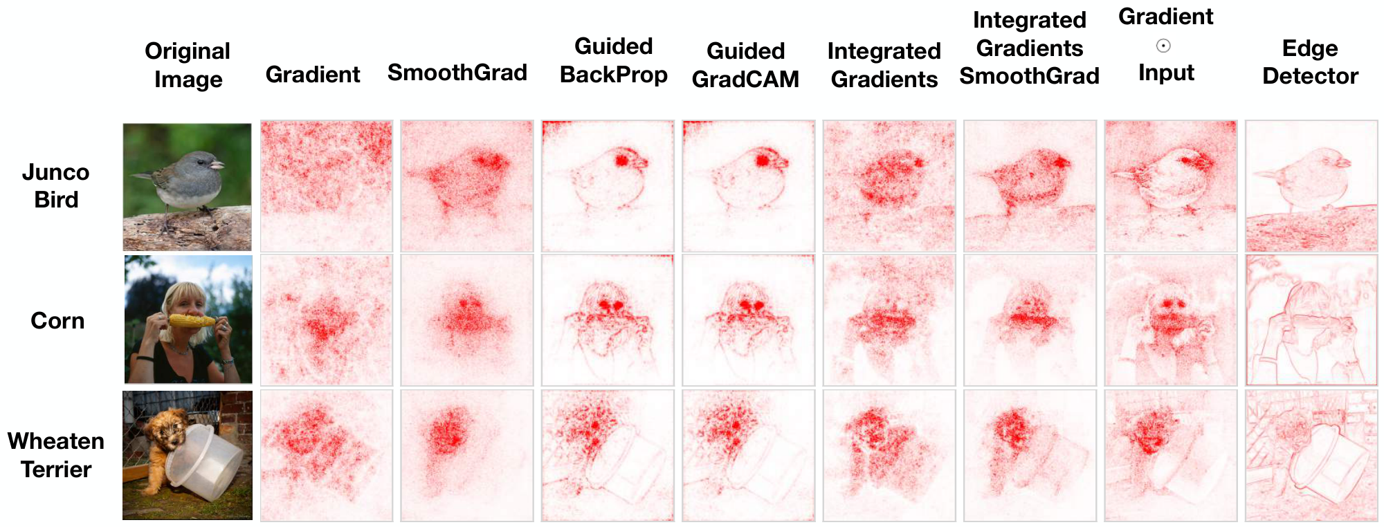
To illustrate the point, Figure 1 compares the output of standard saliency methods with those of an edge detector. The edge detector does not depend on model or training data, and yet produces results that bear visual similarity with saliency maps. This goes to show that visual inspection is a poor guide in judging whether an explanation is sensitive to the underlying model and data.

Our methodology derives from the idea of a statistical randomization test, comparing the natural experiment with an artificially randomized experiment. We focus on two instantiations of our general framework: a model parameter randomization test, and a data randomization test.

The model parameter randomization test compares the output of a saliency method on a trained model with the output of the saliency method on a randomly initialized untrained network of the same architecture. If the saliency method depends on the learned parameters of the model, we should expect its output to differ substantially between the two cases. Should the outputs be similar, however, we can infer that the saliency map is insensitive to properties of the model, in this case, the model parameters. In particular, the output of the saliency map would not be helpful for tasks such as model debugging that inevitably depend on the model.

The data randomization test compares a given saliency method applied to a model trained on a labeled data set with the method applied to the same model architecture but trained on a copy of the data set in which we randomly permuted all labels. If a saliency method depends on the labeling of the data, we should again expect its outputs to differ significantly in the two cases. An insensitivity to the permuted labels, however, reveals that the method does not depend on the relationship between instances (e.g. images) and labels that exists in the original data.

Speaking more broadly, any explanation method admits a set of invariances, i.e., transformations of data and model that do not change the output of the method. If we discover an invariance that is incompatible with the requirements of the task at hand, we can safely reject the method. As such, our tests can be thought of as sanity checks to perform before deploying a method in practice.

Our contributions

1. We propose two concrete, easy to implement tests for assessing the

scope and quality of explanation methods: the model parameter randomization test, and the data randomization test. Both tests applies broadly to explanation methods.

2. We conduct extensive experiments with several explanation methods across

data sets and model architectures, and find, consistently, that some of the methods tested are independent of both the model parameters and the labeling of the data that the model was trained on.

3. Of the methods tested, Gradients & GradCAM pass the sanity checks, while Guided BackProp & Guided GradCAM are invariant to higher layer parameters; hence, fail.

4. Consequently, our findings imply that the saliency methods that fail our proposed tests are incapable of supporting tasks that require explanations that are faithful to the model or the data generating process.

5. We interpret our findings through a series of analyses of

linear models and a simple $1$-layer convolutional sum-pooling architecture, as well as a comparison with edge detectors.

2. Methods and Related Work

Section Summary: This section outlines the basic framework for machine learning explanations, where inputs are data vectors fed into models that predict class labels, and various methods generate "explanation maps" highlighting which input features matter most for predictions. It describes key techniques like gradient-based explanations, which show how small input changes affect outputs, along with variations such as Integrated Gradients to handle issues like saturation, Guided Backpropagation for refined gradients in neural networks, and SmoothGrad to reduce noise by averaging over perturbed inputs. The discussion also touches on related research, including vulnerabilities in these methods, existing evaluation approaches like perturbation tests and localization tasks, and tools for visualizing and comparing explanations using metrics that assess visual similarity.

In our formal setup, an input is a vector $x\in\mathbb{R}^d$. A model describes a function $S\colon\mathbb{R}^d\to\mathbb{R}^C$, where $C$ is the number of classes in the classification problem. An explanation method provides an explanation map $E\colon \mathbb{R}^d\to\mathbb{R}^d$ that maps inputs to objects of the same shape.

We now briefly describe some of the explanation methods we examine. The supplementary materials contain an in-depth overview of these methods. Our goal is not to exhaustively evaluate all prior explanation methods, but rather to highlight how our methods apply to several cases of interest.

The gradient explanation for an input $x$ is $E_{\mathrm{grad}}(x) = \frac{\partial S}{\partial x}$ [22, 23, 8]. The gradient quantifies how much a change in each input dimension would a change the predictions $S(x)$ in a small neighborhood around the input.

Gradient $\odot$ Input. Another form of explanation is the element-wise product of the input and the gradient, denoted $x \odot \frac{\partial S}{\partial x}$, which can address "gradient saturation", and reduce visual diffusion [13].

Integrated Gradients (IG) also addresses gradient saturation by summing over scaled versions of the input [14]. IG for an input $x$ is defined as $E_{\mathrm{IG}}(x) = (x - \bar{x}) \times \int_{0}^1{\frac{\partial S(\bar{x} + \alpha(x-\bar{x}))}{\partial x}} d\alpha, $ where $\bar{x}$ is a "baseline input" that represents the absence of a feature in the original input $x$.

Guided Backpropagation (GBP) [9] builds on the "DeConvNet" explanation method [10] and corresponds to the gradient explanation where negative gradient entries are set to zero while back-propagating through a ReLU unit.

Guided GradCAM. Introduced by [19], GradCAM explanations correspond to the gradient of the class score (logit) with respect to the feature map of the last convolutional unit of a DNN. For pixel level granularity GradCAM, can be combined with Guided Backpropagation through an element-wise product.

SmoothGrad (SG) [16] seeks to alleviate noise and visual diffusion [14, 13] for saliency maps by averaging over explanations of noisy copies of an input. For a given explanation map $E, $ SmoothGrad is defined as $E_{\mathrm{sg}}(x) = \frac{1}{N}\sum_{i=1}^N E(x + g_i), $ where noise vectors $g_i\sim \mathcal{N}(0, \sigma^2)$ are drawn i.i.d. from a normal distribution.

2.1 Related Work

Other Methods & Similarities.

Aside gradient-based approaches, other methods 'learn' an explanation per sample for a model [20, 17, 12, 15, 11, 21]. More recently, [24] showed that for ReLU networks (with zero baseline and no biases) the $\epsilon$-LRP and DeepLift (Rescale) explanation methods are equivalent to the $\text{input} \odot \text{gradient}$. Similarly, [18] proposed SHAP explanations which approximate the shapley value and unify several existing methods.

Fragility.

[25] and [26] both present attacks against saliency methods; showing that it is possible to manipulate derived explanations in unintended ways. [27] theoretically assessed backpropagation based methods and found that Guided BackProp and DeconvNet, under certain conditions, are invariant to network reparamaterizations, particularly random Gaussian initialization. Specifically, they show that Guided BackProp and DeconvNet both seem to be performing partial input recovery. Our findings are similar for Guided BackProp and its variants. Further, our work differs in that we propose actionable sanity checks for assessing explanation approaches. Along similar lines, [28] also showed that some backpropagation-based saliency methods can often lack neuron discriminativity.

Current assessment methods.

Both [29] and [30] proposed an input perturbation procedure for assessing the quality of saliency methods. [17] proposed an entropy based metric to quantify the amount of relevant information an explanation mask captures. Performance of a saliency map on an object localization task has also been used for assessing saliency methods. [30] discuss explanation continuity and selectivity as measures of assessment.

Randomization.

Our label randomization test was inspired by the work of [31], although we use the test for an entirely different purpose.

2.2 Visualization & Similarity Metrics

We discuss our visualization approach and overview the set of metrics used in assessing similarity between two explanations.

Visualization.

We visualize saliency maps in two ways. In the first case, absolute-value (ABS), we take absolute values of a normalized map. For the second case, diverging visualization, we leave the map as is, and use different colors to show positive and negative importance.

Similarity Metrics.

For quantitative comparison, we rely on the following metrics: Spearman rank correlation with absolute value (absolute value), Spearman rank correlation without absolute value (diverging), the structural similarity index (SSIM), and the Pearson correlation of the histogram of gradients (HOGs) derived from two maps. We compute the SSIM and HOGs similarity metric on ImageNet examples without absolute values[^3]. SSIM and Pearson correlation of HOGs have been used in literature to remove duplicate images and quantify image similarity. Ultimately, quantifying human visual perception is still an active area of research.

[^3]: We refer readers to the appendix for a discussion on calibration of these metrics.

3. Model Parameter Randomization Test

Section Summary: This section introduces a test to check if explanation methods for AI models are sensitive to the model's internal parameters, which capture what the model learns from training data and influence its performance. The test involves randomizing the model's weights in two ways—either progressively from the output layers downward in a cascading manner or independently for each layer—and then comparing the resulting explanations to those from the original trained model using metrics like correlation and visual similarity. Key findings show that standard gradient methods detect these changes effectively, especially in higher layers, while methods like Guided Backprop remain largely unaffected until lower layers are altered, highlighting potential pitfalls in relying solely on visual checks.

The parameter settings of a model encode what the model has learned from the data during training. In particular, model parameters have a strong effect on test performance of the model. Consequently, for a saliency method to be useful for debugging a model, it ought to be sensitive to model parameters.

As an illustrative example, consider a linear function of the form $f(x) = w_1x_1 + w_2x_2$ with input $x \in \mathbb{R}^2$. A gradient-based explanation for the model's behavior for input $x$ is given by the parameter values $(w_1, w_2)$, which correspond to the sensitivity of the function to each of the coordinates. Changes in the model parameters therefore change the explanation.

Our proposed model parameter randomization test assesses an explanation method's sensitivity to model parameters. We conduct two kinds of randomization. First we randomly re-initialize all weights of the model both completely and in a cascading fashion. Second, we independently randomize a single layer at a time while keeping all others fixed. In both cases, we compare the resulting explanation from a network with random weights to the one obtained with the model's original weights.

3.1 Cascading Randomization

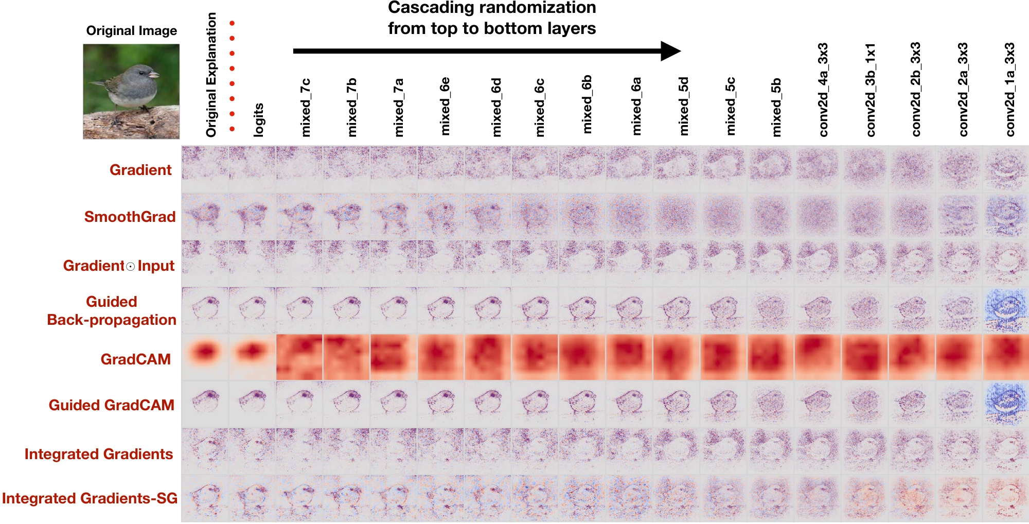
Overview. In the cascading randomization, we randomize the weights of a model starting from the top layer, successively, all the way to the bottom layer. This procedure destroys the learned weights from the top layers to the bottom ones. Figure 2 shows masks, for several saliency methods, for an example input for the cascading randomization on an Inception v3 model trained on ImageNet. In Figure 4, we show the two Spearman (absolute value and no-absolute value) metrics across different data sets and architectures. Finally, in Figure 5, we show the SSIM and HOGs similarity metrics.

The gradient shows sensitivity while Guided Backprop is invariant to higher layer weights. We find that the gradient map is, indeed, sensitive to model parameter randomization. Similarly, GradCAM is sensitive to model weights if the randomization is downstream of the last convolutional layer. However, Guided Backprop (along with Guided GradCAM) is invariant to higher layer weights. Masks derived from Guided Backprop remain visually and quantitatively similar to masks of a trained model until lower layer weights (those closest to the input) are randomized.[^4]

[^4]: A previous version of this work noted that Guided Backprop was entirely invariant; however, this is not this case.

The danger of the visual assessment. On visual inspection, we find that gradient $\odot$ input and integrated gradients show visual similarity to the original mask. In fact, from Figure 2, it is still possible to make out the structure of the bird even after multiple blocks of randomization. This visual similarity is reflected in the SSIM comparison (Figure 5), and the rank correlation with absolute value (Figure 4-Top). However, re-initialization disrupts the sign of the map, so that the spearman rank correlation without absolute values goes to zero (Figure 4-Bottom) almost as soon as the top layers are randomized. The observed visual perception versus ranking dichotomy indicates that naive visual inspection of the masks, in this setting, does not distinguish networks of similar structure but widely differing parameters. We explain the source of this phenomenon in our discussion section.

3.2 Independent Randomization

Overview. As a different form of the model parameter randomization test, we now conduct an independent layer-by-layer randomization with the goal of isolating the dependence of the explanations by layer. This approach allows us to exhaustively assess the dependence of saliency masks on lower versus higher layer weights. More concretely, for each layer, we fix the weights of other layers to their original values, and randomize one layer at a time.

Results. Figure 3 shows the evolution of different masks as each layer of Inception v3 is independently randomized. We observe a correspondence between the results from the cascading and independent layer randomization experiments: Guided Backprop (along with Guided GradCAM) show invariance to higher layer weights. However, once the lower layer convolutional weights are randomized, the Guided Backprop masks changes, although the resulting mask is still dominated by the input structure.

4. Data Randomization Test

Section Summary: The data randomization test examines whether AI explanation methods truly capture the connection between data inputs, like images, and their correct labels by scrambling the labels during model training. This forces the model to memorize random assignments instead of learning real patterns, resulting in poor test performance, and researchers then compare explanations generated by the original model versus this flawed one. Results show that some techniques, such as gradients, change dramatically, while others like Guided BackProp produce visually plausible but misleading highlights even on randomized data, underscoring the risk of relying solely on appearance to validate explanations.

The feasibility of accurate prediction hinges on the relationship between instances (e.g., images) and labels encoded by the data. If we artificially break this relationship by randomizing the labels, no predictive model can do better than random guessing. Our data randomization test evaluates the sensitivity of an explanation method to the relationship between instances and labels. An explanation method insensitive to randomizing labels cannot possibly explain mechanisms that depend on the relationship between instances and labels present in the data generating process. For example, if an explanation did not change after we randomly assigned diagnoses to CT scans, then evidently it did not explain anything about the relationship between a CT scan and the correct diagnosis in the first place (see [32] for an application of Guided BackProp as part of a pipepline for shadow detection in 2D Ultrasound).

In our data randomization test, we permute the training labels and train a model on the randomized training data. A model achieving high training accuracy on the randomized training data is forced to memorize the randomized labels without being able to exploit the original structure in the data. As it turns out, state-of-the art deep neural networks can easily fit random labels as was shown in [31].

In our experiments, we permute the training labels for each model and data set pair, and train the model to greater than $95%$ training set accuracy. Note that the test accuracy is never better than randomly guessing a label (up to sampling error). For each resulting model, we then compute explanations on the same test bed of inputs for a model trained with true labels and the corresponding model trained on randomly permuted labels.

Gradient is sensitive. We find, again, that gradients, and its smoothgrad variant, undergo substantial changes. We also observe that GradCAM masks undergo changes that result in masks with disconnected patches.

Sole reliance on the visual inspection can be misleading. For Guided BackProp, we observe a visual change; however, we find that the masks still highlight portions of the input that would seem plausible, given correspondence with the input, on naive visual inspection. For example, from the diverging masks (Figure 6-Right), we see that the Guided BackProp mask still assigns positive relevance across most of the digit for the network trained on random labels.

For gradient $\odot$ input and integrated gradients, we also observe visual changes in the masks obtained, particularly, in the sign of the attributions. Despite this, the input structure is still clearly prevalent in the masks. The effect observed is particularly prominent for sparse inputs like MNIST where most of the input is zero; however, we observe similar effects for Fashion MNIST (see Appendix), which is less sparse. With visual inspection alone, it is not inconceivable that an analyst could confuse the integrated gradient and gradient $\odot$ input masks derived from a network trained on random labels as legitimate. We clarify these findings and address implications in the discussion section.

5. Discussion

Section Summary: The discussion reflects on how the structure of neural networks shapes the explanations they produce, noting that even untrained models embed useful priors like denoising abilities, though explanations relying solely on architecture may limit their broader usefulness. It examines methods that multiply inputs by gradients, finding that noisy gradients make these explanations resemble the input itself more than meaningful insights, especially for sparse data. Finally, analyzing simple models reveals that saliency techniques work intuitively on linear models by highlighting sensitivities, but on basic convolutional networks, they often detect edges in misleading ways akin to edge filters.

We now take a step back to interpret our findings. First, we discuss the influence of the model architecture on explanations derived from NNs. Second, we consider methods that approximate an element-wise producet of the input and the gradient, as several local explanations do [33, 18]. We show, empirically, that the input "structure" dominates the gradient, especially for sparse inputs. Third, we explain the observed behavior of the gradient explanation with an appeal to linear models. We then consider a single 1-layer convolution with sum-pooling architecture, and show that saliency explanations for this model mostly capture edges. Finally, we return to the edge detector and make comparisons between methods that fail our sanity checks and an edge detector.

5.1 The role of model architecture as a prior

The architecture of a deep neural network has an important effect on the representation derived from the network. A number of results speak to the strength of randomly initialized models as classification priors [34, 35]. Moreover, randomly initialized networks trained on a single input can perform tasks like denoising, super-resolution, and in-painting [36] without additional training data. These prior works speak to the fact that randomly initialized networks correspond to non-trivial representations. Explanations that do not depend on model parameters or training data might still depend on the model architecture and thus provide some useful information about the prior incorporated in the model architecture. However, in this case, the explanation method should only be used for tasks where we believe that knowledge of the model architecture on its own is sufficient for giving useful explanations.

5.2 Element-wise input-gradient products

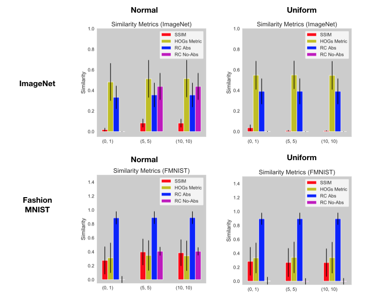
A number of methods, e.g., $\epsilon$-LRP, DeepLift, and integrated gradients, approximate the element-wise product of the input and the gradient (on a piecewise linear function like ReLU). To gain further insight into our findings, we can look at what happens to the input-gradient product $E(x) = x\odot {\frac{\partial S}{\partial x}}, $ if the input is kept fixed, but the gradient is randomized. To do so, we conduct the following experiment. For an input $x$, sample two normal random vectors $u, v$ (we consider both the truncated normal and uniform distributions) and consider the element-wise product of $x$ with $u$ and $v, $ respectively, i.e., $x\odot u$, and $x\odot v$. We then look at the similarity, for all the metrics considered, between $x \odot u$ and $x\odot v$ as noise increases. We conduct this experiment on Fashion MNIST and ImageNet samples. We observe that the input does indeed dominate the product (see Figure 19 in Appendix). We also observe that the input dominance persists even as the noisy gradient vectors change drastically. This experiment indicates that methods that approximate the "input-times-gradient" mostly return the input, in cases where the gradients look visually noisy as they tend to do.

5.3 Analysis for simple models

To better understand our findings, we analyze the output of the saliency methods tested on two simple models: a linear model and a $1$-layer sum pooling convolutional network. We find that the output of the saliency methods, on a linear model, returns a coefficient that intuitively measures the sensitivity of the model with respect to that variable. However, these methods applied to a random convolution seem to result in visual artifacts that are akin to an edge detector.

Linear Model.

Consider a linear model $f: \mathbb{R}^d \rightarrow \mathbb{R}$ defined as $f(x) = w \cdot x$ where $w \in \mathbb{R}^d$ are the model weights. For gradients we have $E_{\mathrm{grad}}(x) = \frac{\partial (w \cdot x)}{ \partial x} = w.$ Similarly for SmoothGrad we have $E_{\mathrm{sg}}(x) = w$ (the gradient is independent of the input, so averaging gradients over noisy inputs yields the same model weight). Integrated Gradients reduces to "gradient $\odot$ input" for this case:

$ \begin{align*} E_{IG}(x) & = (x - \bar{x}) \odot\int_{0}^1{\frac{\partial f(\bar{x} + \alpha(x-\bar{x}))}{\partial x}} d\alpha & = (x - \bar{x}) \odot \int_0^{1} w \alpha d\alpha & = (x - \bar{x}) \odot w/2, . \end{align*} $

Consequently, we see that the application of the basic gradient method to a linear model will pass our sanity check. Gradients on a random model will return an image of white noise, while integrated gradients will return a noisy version of the input image. We did not consider Guided Backprop and GradCAM here because both methods are not defined for the linear model considered above.

1 Layer Sum-Pool Conv Model.

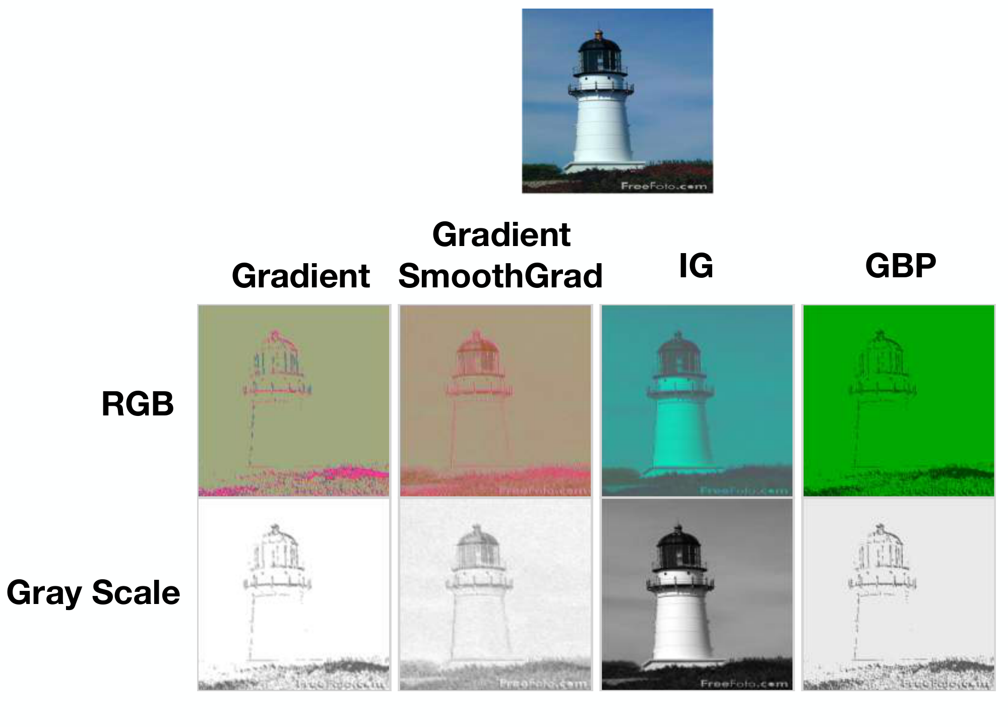
We now show that the application of these same methods to a $1$-layer convolutional network may result in visual artifacts that can be misleading unless further analysis is done. Consider a single-layer convolutional network applied to a grey-scale image $x \in \mathbb{R}^{n \times n}$. Let $w \in \mathbb{R}^{3 \times 3}$ denote the $3 \times 3$ convolutional filter, indexed as $w_{ij}$ for $i, j \in {-1, 0, 1}$. We denote by $w * x \in \mathbb{R}^{n \times n}$ the output of the convolution operation on the image $x$. Then the output of this network can be written as $ l(x) = \sum\limits_{i=1}^{n}\sum\limits_{j=1}^{n} \sigma (w * x)_{ij}, , $ where $\sigma$ is the ReLU non-linearity applied point-wise. In particular, this network applies a single 3x3 convolutional filter to the input image, then applies a ReLU non-linearity and finally sum-pools over the entire convolutional layer for the output. This is a similar architecture to the one considered in [34]. As shown in Figure 7, we see that different saliency methods do act like edge detectors. This suggests that the convolutional structure of the network is responsible for the edge detecting behavior of some of these saliency methods.

To understand why saliency methods applied to this simple architecture visually appear to be edge detectors, we consider the closed form of the gradient $\frac{\partial}{\partial x_{ij}} l(x)$. Let $a_{ij} = \mathbf{1}\left{(w * x)_{ij} \geq 0\right}$ indicate the activation pattern of the ReLU units in the convolutional layer. Then for $i, j \in [2, n-1]$ we have

$ \frac{\partial}{\partial x_{ij}} l(x) = \sum\limits_{k=-1}^{1}\sum\limits_{l=-1}^{1} \sigma'((w * x){i+k, j+l}) w{kl} = \sum\limits_{k=-1}^{1}\sum\limits_{l=-1}^{1} a_{i+k, j+l} w_{kl} $

(Recall that $\sigma'(x) = 0$ if $x < 0$ and $1$ otherwise). This implies that the $3 \times 3$ activation pattern local to pixel $x_{ij}$ uniquely determines $\frac{\partial}{\partial x_{ij}}$. It is now clear why edges will be visible in the produced saliency mask — regions in the image corresponding to an "edge" will have a distinct activation pattern from surrounding pixels. In contrast, pixel regions of the image which are more uniform will all have the same activation pattern, and thus the same value of $\frac{\partial}{\partial x_{ij}}l(x)$. Perhaps a similar principle applies for stacked convolutional layers.

5.4 The case of edge detectors.

An edge detector, roughly speaking, is a classical tool to highlight sharp transitions in an image. Notably, edge detectors are typically untrained and do not depend on any predictive model. They are solely a function of the given input image. As some of the saliency methods we saw, edge detection is invariant under model and data transformations.

In Figure 1 we saw that edge detectors produce images that are strikingly similar to the outputs of some saliency methods. In fact, edge detectors can also produce pictures that highlight features which coincide with what appears to be relevant to a model's class prediction. However, here the human observer is at risk of confirmation bias when interpreting the highlighted edges as an explanation of the class prediction. In Figure 34 (Appendix), we show a qualitative comparison of saliency maps of an input image with the same input image multiplied element-wise by the output of an edge detector. The result indeed looks strikingly similar, illustrating that saliency methods mostly use the edges of the image.

While edge detection is a fundamental and useful image processing technique, it is typically not thought of as an explanation method, simply because it involves no model or training data. In light of our findings, it is not unreasonable to interpret some saliency methods as implicitly implementing unsupervised image processing techniques, akin to edge detection, segmentation, or denoising. To differentiate such methods from model-sensitive explanations, visual inspection is insufficient.

6. Conclusion and future work

Section Summary: This research aims to help scientists evaluate methods that explain how AI models work, suggesting they act as basic checks when creating new ones. The findings reveal that simply looking at these explanations visually can mislead people toward flashy but unreliable approaches that don't truly reflect the model's reasoning or the data it uses. The study highlights how testing for consistency under changes, like randomizing the model or labels, can spot weak methods, and it calls for exploring more tests to build better standards for future AI explanations.

The goal of our experimental method is to give researchers guidance in assessing the scope of model explanation methods. We envision these methods to serve as sanity checks in the design of new model explanations. Our results show that visual inspection of explanations alone can favor methods that may provide compelling pictures, but lack sensitivity to the model and the data generating process.

Invariances in explanation methods give a concrete way to rule out the adequacy of the method for certain tasks. We primarily focused on invariance under model randomization, and label randomization. Many other transformations are worth investigating and can shed light on various methods we did and did not evaluate. Along these lines, we hope that our paper is a stepping stone towards a more rigorous evaluation of new explanation methods, rather than a verdict on existing methods.

Acknowledgments

We thank the Google PAIR team for open source implementation of the methods used in this work. We thank Martin Wattenberg and other members of the Google Brain team for critical feedback and helpful discussions that helped improved the work. Lastly, we thank anonymous reviewers for feedback that helped improve the manuscript. We are also grateful to Leon Sixt for pointing out a bug in our Guided Backprop experiments in an earlier version of this work.

Appendix

Appendix

Section Summary: This appendix provides an overview of various techniques, called saliency or explanation methods, used to understand how neural networks make decisions in image classification tasks by highlighting which parts of the input data matter most. It describes methods like simple input gradients, combinations with input values, modified backpropagation to focus on positive signals, visualization tools for convolutional layers, and ways to smooth or integrate gradients for more reliable insights. The second part outlines the experiments, including models trained on datasets like ImageNet and MNIST, plus tests that randomize model parameters or labels to assess the methods' robustness.

A. Explanation Methods

We now provide additional overview of the different saliency methods that we assess in this work. As described in the main text, an input is a vector $x\in\mathbb{R}^d$. A model describes a function $S\colon\mathbb{R}^d\to\mathbb{R}^C$, where $C$ is the number of classes in the classification problem. An explanation method provides an explanation map $E\colon \mathbb{R}^d\to\mathbb{R}^d$ that maps inputs to objects of the same shape. Each dimension then correspond to the 'relevance' or 'importance' of that dimension to the final output, which is often a class-specific score as specified above.

A.1 Gradient with respect to input

This corresponds to the gradient of the scalar logit for a particular class wrt to the input.

$ \boxed{E_{\mathrm{grad}}(x) = \frac{\partial S}{\partial x}} $

A.2 Gradient $\odot$ Input

Gradient element-wise product with the input. Ancona et. al. show that this input gradient product is equivalent to DeepLift, and $\epsilon$-LRP (other explanations methods), for a network with with only Relu(s) and no additive biases.

$ \boxed{E_{\mathrm{grad \odot input}}(x) = x \odot \frac{\partial S}{\partial x}} $

A.3 Guided Backpropagation (GBP)

GBP specifies a change in how to back-propagate gradienst for ReLus. Let ${f^l, f^{l-1}, ..., f^0}$ be the feature maps derived during the forward pass through a DNN, and ${R^l, R^{l-1}, ..., R^0}$ be `intermediate representations' obtained during the backward pass. Concretely, $f^{l} = relu(f^{l-1}) = max(f^{l-1}, 0), $ and $R^{l+1} = \frac{\partial f^{out}}{\partial f^{l+1}}$ (for regular back-propagation). GBP aims to zero out negative gradients during computation of $R.$ The mask is computed as:

$ \boxed{R^l = 1_{R^{l+1} > 0}1_{f^l > 0} R^{l+1}} $

$1_{R^{l+1} > 0}$ means keep only the positive gradients, and $1_{f^l > 0}$ means keep only the positive activations.

A.4 GradCAM and Guided GradCAM

Introduced by [19], GradCAM explanations correspond to the gradient of the class score (logit) with respect to the feature map of the last convolutional unit of a DNN. For pixel level granularity GradCAM, can be combined with Guided Backpropagation through an element-wise product.

Following the exact notation by [19], let $A^k$ be the feature maps derived from the last convolutional layer of a DNN. Consequently, GradCAM is defined as follows: first, neuron importance weights are calculated, $\alpha_{c}^k = \frac{1}{Z} \sum_{i} \sum_{j} \frac{\partial S}{\partial A_{ij}^k}$, then the GradCAM mask corresponds to: $ReLU(\sum_{k} \alpha_{c}^k A^k)$. This corresponds to a global average pooling of the gradients followed by weighted linear combination to which a ReLU is applied. Now, the Guided GradCAM mask is then defined as:

$ \boxed{E_{\mathrm{guided-gradcam}}(x) = E_{\mathrm{gradcam}}\odot E_{\mathrm{gbp}}} $

A.5 Integrated Gradients (IG)

IG is defined as:

$ \boxed{E_{\mathrm{IG}}(x) = (x - \bar{x}) \times \int_{0}^1{\frac{\partial S(\bar{x} + \alpha(x-\bar{x})}{\partial x}} d\alpha} $

where $\bar{x}$ is the baseline input that represents the absence of a feature in the original sample $x_t$. $\bar{x}$ is typically set to zero.

A.6 SmoothGrad

Given an explanation, $E$, from one of the methods previously discussed, a sample $x$, the SmoothGrad explanation, $E_{\mathrm{sg}}$, is defined as follows:

$ \boxed{E_{\mathrm{sg}}(x) = \frac{1}{N}\sum_{i=1}^N E(x + g_i), } $

where noise vectors $g_i\sim \mathcal{N}(0, \sigma^2))$ are drawn i.i.d. from a normal distribution.

A.7 VarGrad

Similar to SmoothGrad, and as referenced in [37] a variance analog of SmoothGrad can be defined as follows:

$ \boxed{E_{\mathrm{vg}}(x) = \mathcal{V}(E(x + g_i)), } $

where noise vectors $g_i\sim \mathcal{N}(0, \sigma^2))$ are drawn i.i.d. from a normal distribution, and $\mathcal{V}$ corresponds to the variance. In the visualizations presented here, explanations with VG correspond to the VarGrad equivalent of such masks. [38] theoretically analyze VarGrad showing that it is independent of the gradient, and captures higher order partial derivatives.

B. DNN Architecture, Training, Randomization & Metrics

Experimental Details

Data sets & Models. We perform our randomization tests on a variety of datasets and models as follows: an Inception v3 model [39] trained on the ImageNet classification dataset [40] for object recognition, a Convolutional Neural Network (CNN) trained on MNIST [41] and Fashion MNIST [42], and a multi-layer perceptron (MLP), also trained on MNIST and Fashion MNIST.

Randomization Tests We perform 2 types of randomizations. For the model parameter randomization tests, we re-initialized the parameters of each of the models with a truncated normal distribution. We replicated these randomization for a uniform distribution and obtain identical results. For the random labels test, we randomize, completely, the training labels for a each-model dataset pair (MNIST and Fashion MNIST) and then train the model to greater than 95 percent training set accuracy. As expected the performance of these models on the tests set is random.

Inception v3 trained on ImageNet. For Inception v3, we used a pre-trained network that is widely distributed with the tensorflow package available at: https://github.com/tensorflow/models/tree/master/research/slim#Pretrained. This model has a $93.9$ top-5 accuracy on the ImageNet test set. For the randomization tests, we re-initialized on a per-block basis. As noted in ([43]), each inception block consists of multiple filters of different sizes. In this case, we randomize all the the filter weights, biases, and batch-norm variables for each inception block. In total, this randomization occurs in 17 phases.

CNN on MNIST and Fashion MNIST. The CNN architecture is as follows: input -

gt;$ conv (5x5, 32) - gt;$ pooling (2x2)- gt;$ conv (5x5, 64) - gt;$ pooling (2x2) - gt;$ fully connected (1024 units) - gt;$ softmax (10 units). We train the model with the ADAM optimizer for 20 thousand iterations. All non-linearities used are ReLU. We also apply weight decay (penalty $0.001$) to the weights of the network. The final test set accuracy of this model is 99.2 percent. For model parameter randomization test, we reinitialize each layer successively or independently depending on the randomization experiment. The weight initialiazation scheme followed was a truncated normal distribution (mean: 0, std: 0.01). We also tried a uniform distribution as well, and found that our results still hold.

MLP trained on MNIST. The MLP architecture is as follows: input -

gt;$ fully connected (2500 units) - gt;$ fully connected (1500 units) - gt;$ fully connected (500 units) - gt;$ fully connected (10 units). We also train this model with the ADAM optimizer for 20 thousand iterations. All non-linearities used are Relu. The final test set accuracy of this model is 98.7 percent. For randomization tests, we reinitialize each layer successively or independently depending on the randomization experiment.

Inception v4 trained on Skeletal Radiograms. We also analyzed an inception v4 model trained on skeletal radiograms obtained as part of the pediatric bone age challenge conducted by the radiological society of north America. This inception v4 model was trained retained the standard original parameters except it was trained with a mixed L1 and L2 loss. In our randomization test as indicated in figure 1, we reinitialize all weights, biases, and variables of the model.

Calibration for Similarity Metrics. As noted in the methods section, we measure the similarity of the saliency masks obtained using the following metrics: Spearman rank correlation with absolute value (absolute value), Spearman rank correlation without absolute value (diverging), the structural similarity index (SSIM), and the Pearson correlation of the histogram of gradients (HOGs) derived from two maps. The SSIM and HOGs metrics are computed for ImageNet explanation masks. We do this because these metrics are suited to natural images, and to avoid the somewhat artificial structure of Fashion MNIST and MNIST images. We conduct two kinds of calibration exercises. First we measure, for each metric, the similarity between an explanation mask and a randomly sampled (Uniform or Gaussian) mask. Second, we measure, for each metric, the similarity between two randomly sampled explanation masks (Uniform or Gaussian). Together, these two tasks allow us to see if high values for a particular metric indeed correspond to meaningfully high values.

We use the skimage HOG function with a (16, 16) pixels per cell. Note that the input to the HOG function is 299 by 229 with the values normalized to [-1, +1]. We also used the skimage SSIM function with a window size of 5. We obtained the gradient saliency maps for 50 images in the ImageNet validation set. We then compare these under the two settings described above; we report the average across these 50 images as the following tuple: (Rank correlation with no absolute value, Rank correlation with absolute value, HOGs Metric, SSIM). The average similarity between the gradient mask and random Gaussian mask is: $(-0.00049, 0.00032, -0.0016, 0.00027)$. We repeat this experiment for Integrated gradient and gradient $\odot$ input and obtained: $(0.00084, 0.00059, 0.0048, 0.00018)$, and $(0.00081, 0.00099, -0.0024, 0.00023)$. We now report results for the above metrics for similarity between two random masks. For uniform distribution [-1, 1], we obtain the following similarity: $(0.00016, -0.0015, 0.078, 0.00076)$. For Gaussian masks with mean zero and unit variance that has been normalized to lie in the range [-1, 1], we obtain the following similarity metric: $(0.00018, 0.00043, -0.0013, 0.00023)$.

C. Additional Figures

We now present additional figures referenced in the main text.

References

[1] Vellido et al. (2012). Making machine learning models interpretable.. In ESANN. pp. 163–172.

[2] Doshi-Velez et al. (2017). Accountability of AI Under the Law: The Role of Explanation. arXiv preprint arXiv:1711.01134.

[3] Goodman, Bryce and Flaxman, Seth (2016). European Union regulations on algorithmic decision-making and a" right to explanation". arXiv preprint arXiv:1606.08813.

[4] Casillas et al. (2013). Interpretability issues in fuzzy modeling. Springer.

[5] Cadamuro et al. (2016). Debugging machine learning models. In ICML Workshop on Reliable Machine Learning in the Wild.

[6] Lakkaraju et al. (2017). Interpretable & Explorable Approximations of Black Box Models. arXiv preprint arXiv:1707.01154.

[7] Wang, Fulton and Rudin, Cynthia (2015). Causal falling rule lists. arXiv preprint arXiv:1510.05189.

[8] Simonyan et al. (2013). Deep inside convolutional networks: Visualising image classification models and saliency maps. arXiv preprint arXiv:1312.6034.

[9] Springenberg et al. (2014). Striving for simplicity: The all convolutional net. arXiv preprint arXiv:1412.6806.

[10] Zeiler, Matthew D and Fergus, Rob (2014). Visualizing and understanding convolutional networks. In European conference on computer vision. pp. 818–833.

[11] Pieter-Jan Kindermans, Kristof T. Schütt, Maximilian Alber, Klaus-Robert Müller, Dumitru Erhan, Been Kim, Sven Dähne (2018). Learning how to explain neural networks: PatternNet and PatternAttribution. International Conference on Learning Representations. https://openreview.net/forum?id=Hkn7CBaTW.

[12] Zintgraf et al. (2017). Visualizing deep neural network decisions: Prediction difference analysis. arXiv preprint arXiv:1702.04595.

[13] Shrikumar et al. (2016). Not just a black box: Learning important features through propagating activation differences. arXiv preprint arXiv:1605.01713.

[14] Sundararajan et al. (2017). Axiomatic attribution for deep networks. arXiv preprint arXiv:1703.01365.

[15] Ribeiro et al. (2016). Why should i trust you?: Explaining the predictions of any classifier. In Proceedings of the 22nd ACM SIGKDD International Conference on Knowledge Discovery and Data Mining. pp. 1135–1144.

[16] Smilkov et al. (2017). Smoothgrad: removing noise by adding noise. arXiv preprint arXiv:1706.03825.

[17] Dabkowski, Piotr and Gal, Yarin (2017). Real time image saliency for black box classifiers. In Advances in Neural Information Processing Systems. pp. 6970–6979.

[18] Lundberg, Scott M and Lee, Su-In (2017). A unified approach to interpreting model predictions. In Advances in Neural Information Processing Systems. pp. 4768–4777.

[19] Selvaraju et al. (2016). Grad-CAM: Why did you say that?. arXiv preprint arXiv:1611.07450.

[20] Fong, Ruth C and Vedaldi, Andrea (2017). Interpretable explanations of black boxes by meaningful perturbation. arXiv preprint arXiv:1704.03296.

[21] Chen et al. (2018). Learning to Explain: An Information-Theoretic Perspective on Model Interpretation. In Proceedings of the 35th International Conference on Machine Learning. pp. 883–892. http://proceedings.mlr.press/v80/chen18j.html.

[22] Baehrens et al. (2010). How to explain individual classification decisions. Journal of Machine Learning Research. 11(Jun). pp. 1803–1831.

[23] Erhan et al. (2009). Visualizing higher-layer features of a deep network. University of Montreal. 1341(3). pp. 1.

[24] Ancona et al. (2017). A unified view of gradient-based attribution methods for Deep Neural Networks. arXiv preprint arXiv:1711.06104.

[25] Ghorbani et al. (2017). Interpretation of Neural Networks is Fragile. arXiv preprint arXiv:1710.10547.

[26] Kindermans et al. (2017). The (Un) reliability of saliency methods. arXiv preprint arXiv:1711.00867.

[27] Nie et al. (2018). A Theoretical Explanation for Perplexing Behaviors of Backpropagation-based Visualizations. In ICML.

[28] Mahendran, Aravindh and Vedaldi, Andrea (2016). Salient deconvolutional networks. In European Conference on Computer Vision. pp. 120–135.

[29] Samek et al. (2017). Evaluating the visualization of what a deep neural network has learned. IEEE transactions on neural networks and learning systems. 28(11). pp. 2660–2673.

[30] Montavon et al. (2017). Methods for interpreting and understanding deep neural networks. Digital Signal Processing.

[31] Chiyuan Zhang et al. (2017). Understanding deep learning requires rethinking generalization. In In Proc. $5$th ICLR.

[32] Meng et al. (2018). Automatic Shadow Detection in 2D Ultrasound.

[33] Marco Ancona et al. (2018). Towards better understanding of gradient-based attribution methods for Deep Neural Networks. In In Proc. $6$th ICLR.

[34] Saxe et al. (2011). On Random Weights and Unsupervised Feature Learning.. In ICML. pp. 1089–1096.

[35] Alain, Guillaume and Bengio, Yoshua (2016). Understanding intermediate layers using linear classifier probes. arXiv preprint arXiv:1610.01644.

[36] Ulyanov et al. (2017). Deep Image Prior. arXiv preprint arXiv:1711.10925.

[37] Adebayo et al. (2018). Local explanation methods for deep neural networks lack sensitivity to parameter values.

[38] Seo et al. (2018). Noise-adding Methods of Saliency Map as Series of Higher Order Partial Derivative. arXiv preprint arXiv:1806.03000.

[39] Szegedy et al. (2016). Rethinking the inception architecture for computer vision. In Proceedings of the IEEE Conference on Computer Vision and Pattern Recognition. pp. 2818–2826.

[40] Russakovsky et al. (2015). Imagenet large scale visual recognition challenge. International Journal of Computer Vision. 115(3). pp. 211–252.

[41] LeCun, Yann (1998). The MNIST database of handwritten digits. http://yann. lecun. com/exdb/mnist/.

[42] Xiao et al. (2017). Fashion-mnist: a novel image dataset for benchmarking machine learning algorithms. arXiv preprint arXiv:1708.07747.

[43] Szegedy et al. (2017). Inception-v4, inception-resnet and the impact of residual connections on learning.. In AAAI. pp. 12.