Transductive Inference for Text Classification using Support Vector Machines

Thorsten Joachims
Universität Dortmund, LS VIII
44221 Dortmund, Germany
[email protected]

Abstract

This paper introduces Transductive Support Vector Machines (TSVMs) for text classification. While regular Support Vector Machines (SVMs) try to induce a general decision function for a learning task, Transductive Support Vector Machines take into account a particular test set and try to minimize misclassifications of just those particular examples. The paper presents an analysis of why TSVMs are well suited for text classification. These theoretical findings are supported by experiments on three test collections. The experiments show substantial improvements over inductive methods, especially for small training sets, cutting the number of labeled training examples down to a twentieth on some tasks. This work also proposes an algorithm for training TSVMs efficiently, handling 10,000 examples and more.

Executive Summary: Organizations face growing volumes of digital text that must be rapidly categorized for search, routing, and filtering. Manually labeling training data to build accurate machine learning models is expensive, time-consuming, and often impractical when categories frequently change or require immediate results. Standard inductive models require large volumes of labeled examples to perform well, creating a significant bottleneck for real-world deployment.

The article evaluates whether Transductive Support Vector Machines can dramatically reduce the need for labeled training data in text classification by directly leveraging the natural cluster structure found within unlabeled test documents.

To demonstrate this, the author developed a scalable local search algorithm capable of training transductive models on datasets with over 10,000 examples. The approach was tested across three diverse benchmark document collections—Reuters newswire articles, WebKB university web pages, and the Ohsumed biomedical database—comparing performance against traditional inductive Support Vector Machines and standard baseline classifiers across varying training set sizes.

The primary finding is that the transductive approach significantly improves classification accuracy when labeled training data is scarce, reducing the required volume of labeled training examples by up to a factor of twenty on certain tasks. For example, on the Reuters dataset with only 17 labeled examples per class, the transductive method raised the average precision-recall breakeven performance from 48.4 to 60.8 compared to standard inductive baselines. The performance advantage is most pronounced when the available unlabeled test collection is large, though the performance difference diminishes as the volume of labeled training data increases. Additionally, the analysis revealed that the method can temporarily struggle if a category has very few positive examples and contains internal topic clusters that mislead the separator.

These results show that organizations can deploy high-performing text classifiers much faster and at substantially lower manual labeling costs. Instead of waiting weeks to collect and annotate large training datasets, systems can deliver strong classification accuracy immediately by analyzing the unlabeled documents they are tasked with sorting.

Decision-makers should consider adopting transductive methods for text processing workflows where unlabeled target documents are readily available but labeled data is minimal, such as reorganizing document databases, filtering incoming feeds, and relevance feedback in search systems. For implementation, teams should run pilot tests to ensure the target categories align well with document cluster patterns and do not suffer from severe class imbalance.

Confidence in these findings is high for standard text classification benchmarks involving large pools of unlabeled documents. However, caution is advised when applying the method to highly imbalanced categories or complex document sets where internal subtopics may divert the decision boundary.

1 Introduction

Section Summary: Text classification has grown essential for tasks like organizing documents, filtering spam, and personalizing news feeds, yet building effective systems from limited labeled examples remains challenging. Rather than inducing a general rule that works across all possible future data, this work focuses on a transductive approach that aims to accurately classify a specific large set of unlabeled examples using only a small training set. To achieve this, the paper introduces transductive support vector machines, which outperform standard SVMs on text tasks and include a new algorithm for efficient training on large collections.

Over the recent years, text classification has become one of the key techniques for organizing online information. It can be used to organize document databases, filter spam from people's email, or learn users' newsreading preferences. Since hand-coding text-classifiers is impractical — or at best costly — in many settings, it is preferable to learn classifiers from examples. It is crucial that the learner be able to generalize well using little training data. A news-filtering service, for example, requiring a hundred days' worth of training data is unlikely to please even the most patient users.

The work presented here tackles the problem of learning from small training samples by taking a transductive [Vapnik, 1998], instead of an inductive approach. In the inductive setting the learner tries to induce a decision function which has a low error rate on the whole distribution of examples for the particular learning task. Often, this setting is unnecessarily complex. In many situations we do not care about the particular decision function, but rather that we classify a given set of examples (i.e. a test set) with as few errors as possible. This is the goal of transductive inference.

Some examples of transductive text classification tasks are the following. All have in common that there is little training data, but a very large test set.

Relevance Feedback : This is a standard technique in free-text information retrieval. The user marks some documents returned by an initial query as relevant or irrelevant. These compose the training set of a text classification task, while the remaining document database is the test set. The user is interested in a good classification of the test set into those documents relevant or irrelevant to the query.

Netnews Filtering : Each day a large number of netnews articles is posted. Given the few training examples the user labeled on previous days, he or she wants today's most interesting articles.

Reorganizing a document collection : With the advance of paperless offices, companies start using document databases with classification schemes. When introducing new categories, they need text classifiers which, given some training examples, classify the rest of the database automatically.

This paper introduces Transductive Support Vector Machines (TSVMs) for text classification. They substantially improve the already excellent performance of SVMs for text classification [Joachims, 1998, Dumais et al., 1998]. Especially for very small training sets, TSVMs reduce the required amount of labeled training data down to a twentieth for some tasks. To facilitate the large-scale transductive learning needed for text classification, this paper also proposes a new algorithm for efficiently training TSVMs with 10,000 examples and more.

2 Text Classification

Section Summary: Text classification uses machine learning to automatically sort documents into a fixed set of semantic categories, treating the task as supervised learning where each category is handled as a separate yes-or-no decision. Documents are first turned into numerical feature vectors by breaking text into word stems, counting how often each stem appears, scaling those counts by inverse document frequency to highlight distinctive terms, and normalizing the vectors to remove effects of varying document length. This representation lets standard learning algorithms decide category membership without needing to consider word order.

The goal of text classification is the automatic assignment of documents to a fixed number of semantic categories. Each document can be in multiple, exactly one, or no category at all. Using machine learning, the objective is to learn classifiers from examples which assign categories automatically. This is a supervised learning problem. To facilitate effective and efficient learning, each category is treated as a separate binary classification problem. Each such problem answers the question of whether or not a document should be assigned to a particular category.

Documents, which typically are strings of characters, have to be transformed into a representation suitable for the learning algorithm and the classification task. Information Retrieval research suggests that word stems work well as representation units and that for many tasks their ordering can be ignored without losing too much information. The word stem is derived from the occurrence form of a word by removing case and inflection information [Porter, 1980]. For example "computes", "computing", and "computer" are all mapped to the same stem "comput". The terms "word" and "word stem" will be used synonymously in the following.

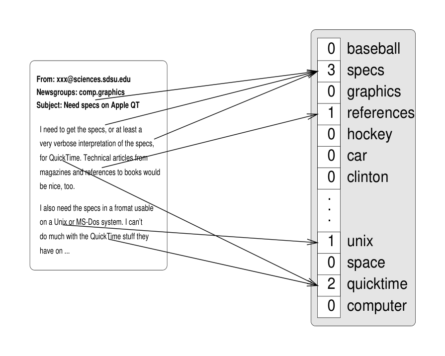
This leads to an attribute-value representation of text. Each distinct word $w_i$ corresponds to a feature with $TF(w_i, x)$, the number of times word $w_i$ occurs in the document $x$, as its value. Figure 1 shows an example feature vector for a particular document. Refining this basic representation, it has been shown that scaling the dimensions of the feature vector with their inverse document frequency $IDF(w_i)$ [Salton and Buckley, 1988] leads to an improved performance. $IDF(w_i)$ can be calculated from the document frequency $DF(w_i)$, which is the number of documents the word $w_i$ occurs in.

$ IDF(w_i) = \log\left(\frac{n}{DF(w_i)}\right)\tag{1} $

Here, $n$ is the total number of documents. Intuitively, the inverse document frequency of a word is low if it occurs in many documents and is highest if the word occurs in only one. To abstract from different document lengths, each document feature vector $\vec{x}_i$ is normalized to unit length.

3 Transductive Support Vector Machines

Section Summary: Transductive support vector machines extend the usual supervised learning setup by providing the algorithm not only with labeled training examples but also with a set of unlabeled test examples drawn from the same distribution. Instead of learning a general decision rule that must work on any future data, the method directly seeks a labeling of those specific test points together with a separating hyperplane that maximizes the margin on both the training and test samples simultaneously. This joint optimization is expressed as a combinatorial problem whose solution corresponds to choosing the equivalence class of hypotheses with the smallest guaranteed test error, and it can be extended to non-separable data by introducing slack variables.

The setting of transductive inference was introduced by Vapnik (see for example [Vapnik, 1998]). For a learning task $P(\vec{x}, y) = P(y|\vec{x})P(\vec{x})$ the learner $L$ is given a hypothesis space $H$ of functions $h : X \to {-1, 1}$ and an i.i.d. sample $S_{\text{train}}$ of $n$ training examples

$ (\vec{x}_1, y_1), (\vec{x}_2, y_2), \dots, (\vec{x}_n, y_n)\tag{2} $

Each training example consists of a document vector $\vec{x} \in X$ and a binary label $y \in {-1, +1}$. In contrast to the inductive setting, the learner is also given an i.i.d. sample $S_{\text{test}}$ of $k$ test examples

$ \vec{x}_1^*, \vec{x}_2^*, \dots, \vec{x}_k^*\tag{3} $

from the same distribution. The transductive learner $L$ aims to selects a function $h_L = L(S_{\text{train}}, S_{\text{test}})$ from $H$ using $S_{\text{train}}$ and $S_{\text{test}}$ so that the expected number of erroneous predictions

$ R(L) = \int \frac{1}{k}\sum_{i=1}^k \Theta(h_L(\vec{x}_i^*), y_i^*) dP(\vec{x}_1, y_1)\dots dP(\vec{x}_k^*, y_k^*) $

on the test examples is minimized. $\Theta(a, b)$ is zero if $a = b$, otherwise it is one. Vapnik [Vapnik, 1998] gives bounds on the relative uniform deviation of training error

$ R_{\text{train}}(h) = \frac{1}{n} \sum_{i=1}^n \Theta(h(\vec{x}_i), y_i)\tag{4} $

and test error

$ R_{\text{test}}(h) = \frac{1}{k} \sum_{i=1}^k \Theta(h(\vec{x}_i^*), y_i^{\text{true}})\tag{5} $

With probability $1 - \eta$

$ R_{\text{test}}(h) \le R_{\text{train}}(h) + \Omega(n, k, d, \eta)\tag{6} $

where the confidence interval $\Omega(n, k, d, \eta)$ depends on the number of training examples $n$, the number of test examples $k$, and the VC-Dimension $d$ of $H$ (see [Vapnik, 1998] for details).

This problem of transductive inference may not seem profoundly different from the usual inductive setting studied in machine learning. One could learn a decision rule based on the training data and then apply it to the test data afterwards. Nevertheless, to solve the problem of estimating $k$ binary values $y_1^*, \dots, y_k^*$ we need to solve the more complex problem of estimating a function over a possibly continuous space. This may not be the best solution when the size $n$ of the training sample (2) is small.

What information do we get from studying the test sample (3) and how can we use it? The training and the test sample split the hypothesis space $H$ into a finite number of equivalence classes $H'$. Two functions from $H$ belong to the same equivalence class if they both classify the training and the test sample in the same way. This reduces the learning problem from finding a function in the possibly infinite set $H$ to finding one of finitely many equivalence classes $H'$. Most importantly, we can use these equivalence classes to build a structure of increasing VC-Dimension for structural risk minimization [Vapnik, 1998].

$ H_1' \subset H_2' \subset \dots \subset H'\tag{7} $

Unlike in the inductive setting, we can study the location of the test examples when defining the structure. Using prior knowledge about the nature of $P(\vec{x}, y)$ we can build a more appropriate structure and learn more quickly. What this means for text classification is analyzed in section 4. In particular, we can build the structure based on the margin of separating hyperplanes on both the training and the test data. Vapnik shows that with the size of the margin we can control the maximum number of equivalence classes (i. e. the VC-Dimension).

Theorem 1 ([Vapnik, 1998])
Consider hyperplanes $h(\vec{x}) = \text{sign}{\vec{x} \cdot \vec{w} + b}$ as hypothesis space $H$. If the attribute vectors of a training sample (2) and a test sample (3) are contained in a ball of diameter $D$, then there are at most

$ N_r < \exp\left(d\left(\frac{n+k}{d} + 1\right)\right), d = \min\left(a, \left[\frac{D^2}{\rho^2}\right] + 1\right) $

equivalence classes which contain a separating hyperplane with

$ \forall_{i=1}^n \left|\frac{\vec{w}}{|\vec{w}|} \cdot \vec{x}i + b\right| \ge \rho \quad \forall{j=1}^k \left|\frac{\vec{w}}{|\vec{w}|} \cdot \vec{x}_j^* + b\right| \ge \rho $

(i.e. margin larger or equal to $\rho$). $a$ is the dimensionality of the space, and $[b]$ is the integer part of $b$.

Note that the VC-Dimension does not necessarily depend on the number of features, but can be much lower than the dimensionality of the space. Let's use this structure based on the margin of separating hyperplanes. Structural risk minimization tells us that we get the smallest bound on the test error if we select the equivalence class from the structure element $H_i'$ which minimizes (6). For linearly separable problems this leads to the following optimization problem [Vapnik, 1998].

OP 1 (Transductive SVM (lin. sep. case))
Minimize over $(y_1^, \dots, y_k^*, \vec{w}, b)$:*

$ \frac{1}{2} |\vec{w}|^2 $

subject to: $\forall_{i=1}^n : y_i[\vec{w} \cdot \vec{x}i + b] \ge 1$
$\forall{j=1}^k : y_j^*[\vec{w} \cdot \vec{x}_j^* + b] \ge 1$

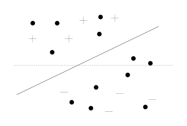
Solving this problem means finding a labelling $y_1^*, \dots, y_k^*$ of the test data and a hyperplane $\langle\vec{w}, b\rangle$, so that this hyperplane separates both training and test data with maximum margin. Figure 2 illustrates this. To be able to handle non-separable data, we can introduce slack variables $\xi_i$ similarly to the way we do with inductive SVMs.

OP 2 (Transductive SVM (non-sep. case))
Minimize over $(y_1^, \dots, y_k^*, \vec{w}, b, \xi_1, \dots, \xi_n, \xi_1^*, \dots, \xi_k^*)$:*

$ \frac{1}{2}|\vec{w}|^2 + C\sum_{i=1}^n \xi_i + C^*\sum_{j=1}^k \xi_j^* $

subject to: $\forall_{i=1}^n : y_i[\vec{w} \cdot \vec{x}i + b] \ge 1 - \xi_i$
$\forall{j=1}^k : y_j^*[\vec{w} \cdot \vec{x}j^* + b] \ge 1 - \xi_j^*$
$\forall{i=1}^n : \xi_i > 0$
$\forall_{j=1}^k : \xi_j^* > 0$

$C$ and $C^*$ are parameters set by the user. They allow trading off margin size against misclassifying training examples or excluding test examples. How this optimization problem can be solved efficiently is the subject of section 4.1.

{width=80%}

4 What Makes TSVMs Especially well Suited for Text Classification?

Section Summary: Text classification involves high-dimensional yet sparse data where most words carry useful information, a setting where support vector machines already perform strongly due to their robustness and resistance to overfitting. Transductive SVMs build on this by also exploiting the natural tendency of words to appear in topic-specific clusters, using the positions of unlabeled test documents to identify those groupings and select a decision boundary that respects them. This lets the method turn co-occurrence patterns in the test set into an inductive bias that improves accuracy beyond what purely inductive learners can achieve from training data alone.

The text classification task is characterized by a special set of properties. They are independent of whether text classification is used for information filtering, relevance feedback, or for assigning semantic categories to news articles.

High dimensional input space:
When learning text classifiers one has to deal with very many (more than 10,000) features, since each (stemmed) word is a feature.

Document vectors are sparse:
For each document, the corresponding document vector $\vec{x}_i$ contains few entries that are not zero.

Few irrelevant features:
Experiments in [Joachims, 1998] suggest that most words are relevant. So aggressive feature selection has to be handled with care, since it can easily lead to a loss of important information[^1].

[^1]: This does not mean that aggressive feature selection cannot be beneficial for certain learning algorithms or certain tasks (see [Yang and Pedersen, 1997][Mladenić, 1998]).

Arguments from [Joachims, 1998] show that SVMs are especially well-suited for this setting, outperforming conventional methods substantially while also being more robust. Dumais et al. [Dumais et al., 1998] come to similar conclusions. TSVMs inherit most properties of SVMs so that the same arguments apply to TSVMs as well.

But how can TSVMs be any better? In the field of information retrieval it is well known that words in natural language occur in strong co-occurrence patterns (see [van Rijsbergen, 1977]). Some words are likely to occur together in one document, others are not. For examples, when asking the search engine Altavista about all documents containing the words pepper and salt, it returns 327,180 web pages. When asking for the documents with the words pepper and physics, we get only 4,220 hits, although physics is a more popular word on the web than salt. Many approaches in information retrieval try to exploit this cluster structure of text (see [van Rijsbergen, 1977]). And it is this co-occurrence information that TSVMs exploit as prior knowledge about the learning task.

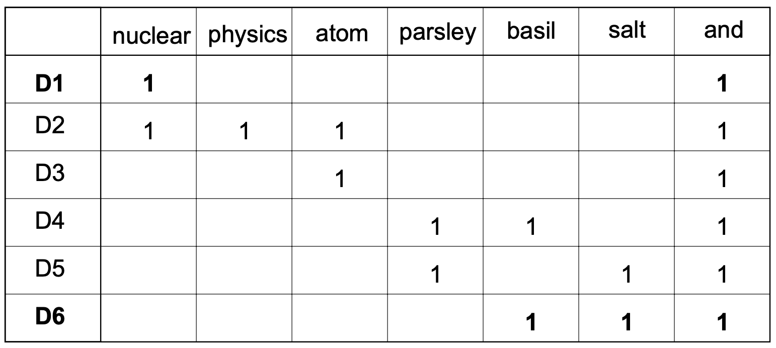
Let's look at the example in figure 3. Imagine document $D1$ was given as a training example for class $A$ and document $D6$ was given as a training example for class $B$. How should we classify documents $D2$ to $D4$ (the test set)? Even if we did not understand the meaning of the words, we would classify $D2$ and $D3$ into class $A$, and $D3$ and $D4$ into class $B$. We would do so even though $D1$ and $D3$ do not share any informative words. The reason we choose this classification of the test data over the others stems from our prior knowledge about the properties of text and common text classification tasks. Often we want to classify documents by topic, source, or style. For these type of classification tasks we find stronger co-occurrence patterns within categories than between different categories. In our example we analyzed the co-occurrence information in the test data and found two clusters. These clusters indicate different topics of ${D1, D2, D3}$ vs. ${D4, D5, D6}$, and we choose the cluster separator as our classification. Note again that we got to this classification by studying the location of the test examples, which is not possible for an inductive learner.

The TSVM outputs the same classification as we suggested above, although all 16 dichotomies of $D2$ to $D5$ can be achieved with linear separators. Assigning $D2$ and $D3$ to class $A$ and $D3$ and $D4$ to class $B$ is the maximum margin solution (i.e. the solution of optimization problem OP1). We see that the maximum margin bias reflects our prior knowledge about text classification well. By analyzing the test set, we can exploit this prior knowledge for learning.

4.1 Solving the Optimization Problem

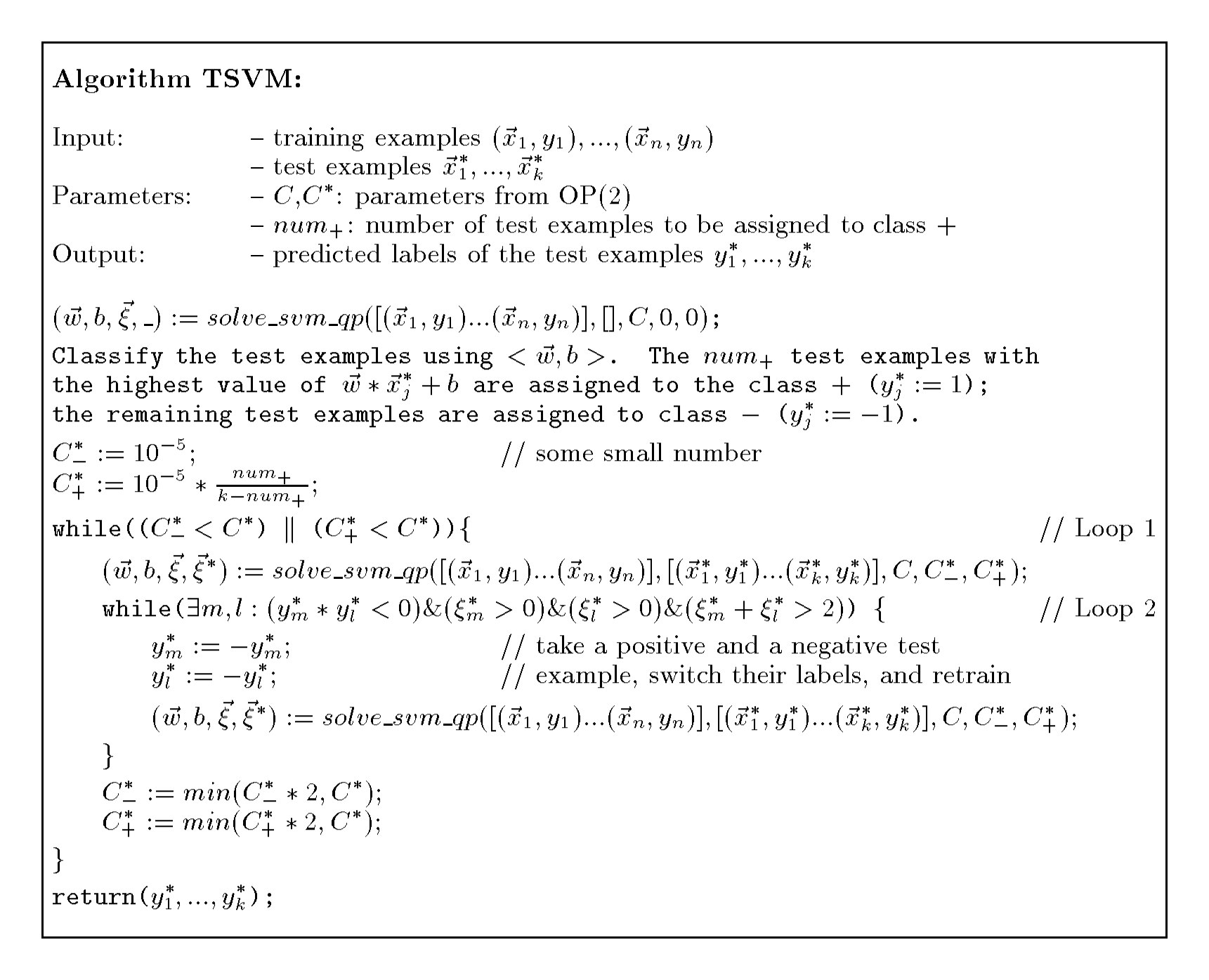
Training a transductive SVM means solving the (partly) combinatorial optimization problem OP2. For a small number of test examples, this problem can be solved optimally simply by trying all possible assignments of $y_1^*, \dots, y_k^*$ to the two classes. However, this approach become intractable for test sets with more than 10 examples. Previous approaches using branch-and-bound search [Wapnik and Tscherwonenkis, 1979] push the limit to some extent, but still lag behind the needs of the text classification problem. The algorithm proposed next is designed to handle the large test sets common in text classification with 10,000 test examples and more. It finds an approximate solution to optimization problem OP2 using a form of local search.

The key idea of the algorithm is that it begins with a labeling of the test data based on the classification of an inductive SVM. Then it improves the solution by switching the labels of test examples so that the objective function decreases. The algorithm takes the training data and the test examples as input and outputs the predicted classification of the test examples. Besides the two parameters $C$ and $C^*$, the user can specify the number of test examples to be assigned to class $+$. This allows trading-off recall vs. precision (see section 5.2). The following description of the algorithm covers only the linear case. A generalization to non-linear hypothesis spaces using kernels is straightforward.

The algorithm is summarized in figure 4. It starts with training an inductive SVM on the training data and classifying the test data accordingly. Then it uniformly increases the influence of the test examples by incrementing the cost-factors $C_-^*$ and $C_+^*$ up to the user defined value of $C^*$ (loop 1). The algorithm uses unbalanced costs $C_-^*$ and $C_+^*$ to better accomodate the user defined ratio $num_+$. While the criterion in the condition of loop 2 identifies two examples for which changing the class labels leads to a decrease in the current objective function, these examples are switched.

The function solve_svm_qp refers to quadratic programs of the following type.

OP 3 (Inductive SVM (primal))
Minimize over $(\vec{w}, b, \vec{\xi}, \vec{\xi}^)$:*

$ \frac{1}{2}|\vec{w}|^2 + C\sum_{i=1}^n \xi_i + C_-^* \sum_{j:y_j^*=-1} \xi_j^* + C_+^* \sum_{j:y_j^*=1} \xi_j^* $

subject to: $\forall_{i=1}^n : y_i[\vec{w} \cdot \vec{x}i + b] \ge 1 - \xi_i$
$\forall{j=1}^k : y_j^*[\vec{w} \cdot \vec{x}_j^* + b] \ge 1 - \xi_j^*$

This optimization problem can be solved in its dual formulation using $SVM^{\text{light}}$ [Joachims, 1999][^2]. Especially designed for text classification, $SVM^{\text{light}}$ can efficiently handle problems with many thousand support vectors, converges fast, and has minimal memory requirements. Let's finally look at an algorithmic property of the algorithm before evaluating its performance empirically in section 5.

[^2]: Available at http://www-ai.cs.uni-dortmund.de/svm_light

Theorem 2 Algorithm 1 converges in a finite number of steps.

Proof: To prove this, it is necessary to show that loop 2 is exited after a finite number of iterations. This holds since the objective function of optimization problem OP2 decreases with every iteration of loop 2 as the following argument shows. The condition $y_m^* y_l^* < 0$ in loop 2 requires that the examples to be switched have different class labels. Let $y_m^* = 1$ so that we can write

$ \frac{1}{2}|\vec{w}|^2 + C\sum_{i=0}^n \xi_i + C_-^* \sum_{j:y_j^*=-1} \xi_i^* + C_+^* \sum_{j:y_j^*=1} \xi_i^* $

$ = \frac{1}{2}|\vec{w}|^2 + C\sum_{i=0}^n \xi_i + \dots + C_+^* \xi_m^* + \dots + C_-^* \xi_l^* + \dots $

$

\frac{1}{2}|\vec{w}|^2 + C\sum_{i=0}^n \xi_i + \dots + C_-^*(2 - \xi_m^*) + \dots + C_+^*(2 - \xi_l^*) + \dots $

$ = \frac{1}{2}|\vec{w}|^2 + C\sum_{i=0}^n \xi_i + \dots + C_-^* {\xi_m^*}' + \dots + C_+^* {\xi_l^*}' + \dots $

It is easy to verify that the constraints of OP2 are fulfilled for the new values of $y_m^*$, $y_l^*$, ${\xi_m^*}'$, and ${\xi_l^*}'$ (potentially, after setting negative ${\xi_m^*}'$ or ${\xi_l^*}'$ to zero). The inequality holds due to the selection criterion in loop 2, since ${\xi_m^*}' = \max(2 - \xi_m^*, 0) < \xi_l^*$ and ${\xi_l^*}' = \max(2 - \xi_l^*, 0) < \xi_m^*$. This means that loop 2 is exited after a finite number of iterations, since there is only a finite number of permutations of the test examples. Loop 1 also terminates after a finite number of iterations, since $C^*$ is bounded by $C^*$. $\square$

5 Experiments

Section Summary: The experiments evaluate transductive support vector machines on three standard text classification collections—Reuters news articles, CMU web pages, and Ohsumed medical abstracts—using the precision/recall breakeven point as the performance measure for documents that may belong to multiple categories. Results compare the transductive approach against an inductive SVM and a multinomial Naive Bayes classifier across varying training and test set sizes. The transductive method consistently improves accuracy, with the largest gains occurring when labeled training data is scarce and when larger unlabeled test sets are available.

5.1 Test Collections

The empirical evaluation is done on three test collection. The first one is the Reuters-21578 dataset[^3] collected from the Reuters newswire in 1987. The "ModApte" split is used, leading to a corpus of 9,603 training documents and 3,299 test documents. Of the 135 potential topic categories only the most frequent 10 are used, while keeping all documents. Both stemming and stop-word removal are used.

[^3]: Available at http://www.research.att.com/~lewis/reuters21578.html

The second dataset is the WebKB collection[^4] of WWW pages made available by the CMU text-learning group. Following the setup in [Nigam et al., 1998], only the classes course, faculty, project, and student are used. Documents not in one of these classes are deleted. After removing documents which just contain the relocation command for the browser, this leaves 4,183 examples. The pages from Cornell University are used for training, while all other pages are used for testing. Like in [Nigam et al., 1998], stemming and stop-word removal are not used.

[^4]: Available at http://www.cs.cmu.edu/afs/cs/project/theo-20/www/data

The third test collection is taken from the Ohsumed corpus[^5] compiled by William Hersh. From the 50,216 documents in 1991 which have abstracts, the first 10,000 are used for training and the second 10,000 are used for testing. The task is to assign documents to one or multiple categories of the 5 most frequent MeSH "diseases" categories. A document belongs to a category if it is indexed with at least one indexing term from that category. Both stemming and stop-word removal are used.

[^5]: Available at ftp://medir.ohsu.edu/pub/ohsumed

5.2 Performance Measures

Since for both the Reuters dataset and the Ohsumed collection documents can be in multiple categories, the Precision/Recall-Breakeven Point is used as a measure of performance. The P/R-breakeven point is a common measure for evaluating text classifiers. It is based on the two well know statistics recall and precision widely used in information retrieval. Precision is the probability that a document predicted to be in class "+" truly belongs to this class. Recall is the probability that a document belonging to class "+" is classified into this class (see [Raghavan et al., 1989]). Both can be estimated from the contingency table.

Between high recall and high precision exists a trade-off. The P/R-breakeven point is defined as that value for which precision and recall are equal. The transductive SVM uses the breakeven point for which the number of false positives equals the number of false negatives. For the inductive SVM and the Naive Bayes classifier the breakeven point is computed by varying the threshold on their "confidence value".

5.3 Results

The following experiments show the effect of using the transductive SVM instead of inductive methods. To provide a baseline for comparison, the results of the inductive SVM and a multinomial Naive Bayes classifier as described in [Joachims, 1997, McCallum and Nigam, 1998] are added. Where applicable, the results are averaged over a number of random training (test) samples.

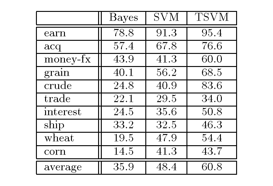
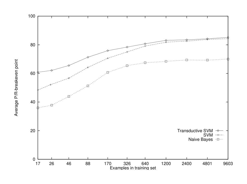
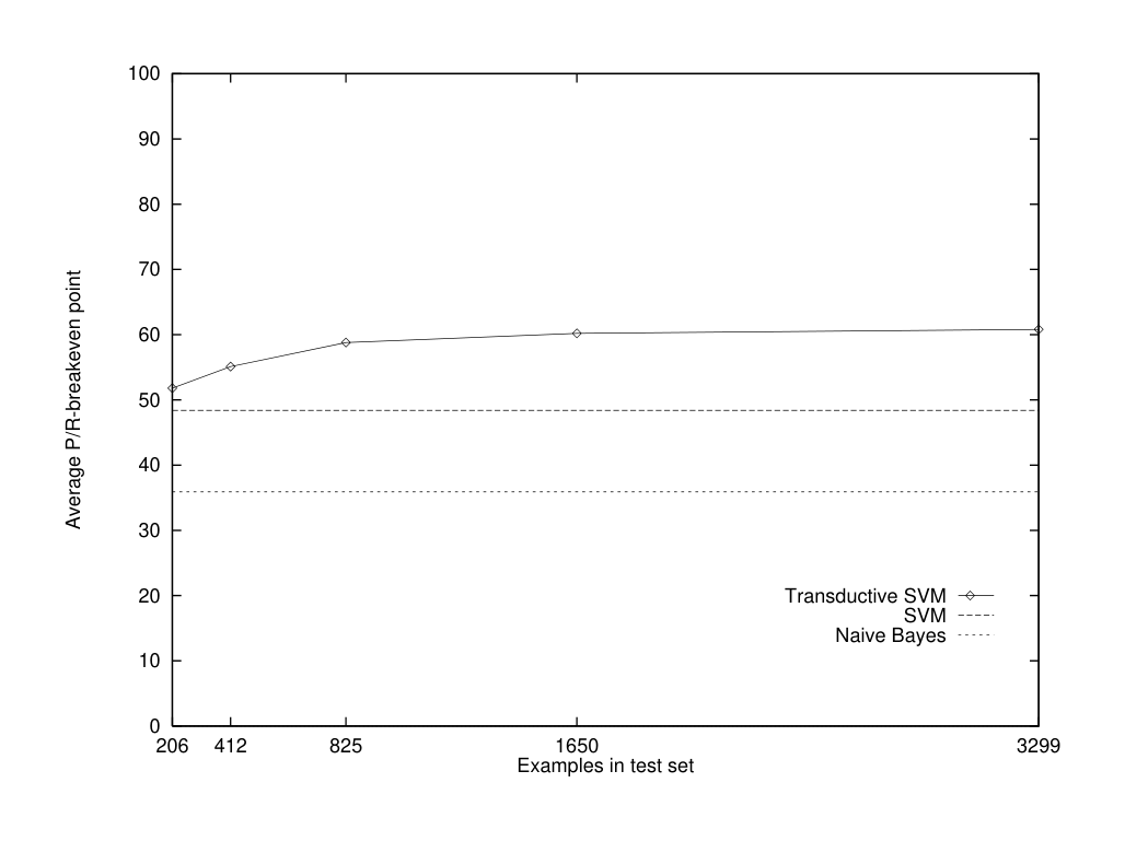
Figure 5 gives the results for the Reuters dataset. For training sets of 17 documents and test sets of 3,299 documents, the transductive SVM leads to an improved performance on all categories, raising the average of the P/R-breakeven points from 48.4 for the inductive SVM to 60.8. These averages correspond to the left-most points in figure 6. This graph shows the effect of varying the size of the training set. The advantage of using the transductive approach is largest for small training sets. For increasing training set size, the performance of the SVM approaches that of the TSVM. The influence of the test set size on the performance of the TSVM is displayed in figure 7. The bigger the test set, the larger the performance gap between SVM and TSVM. Adding more test examples beyond 3,299 is not likely to increase performance by much, since the graph is already very flat.

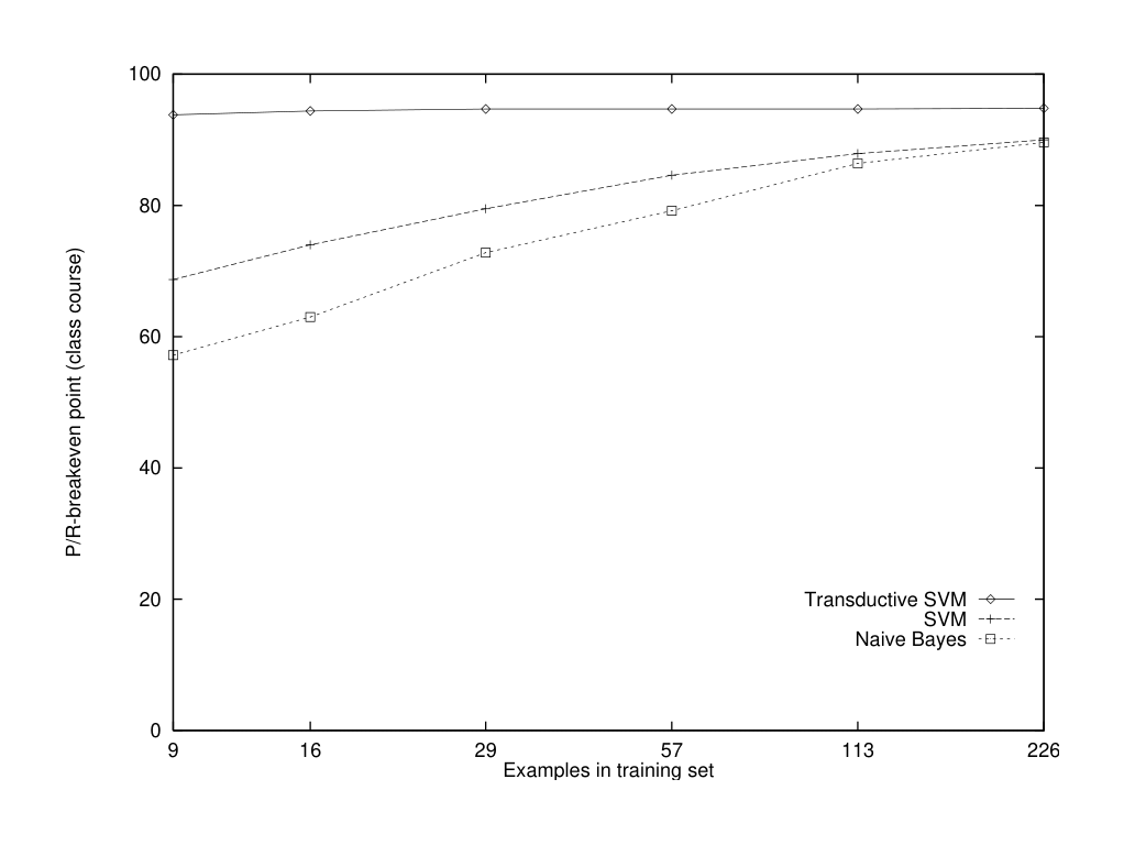
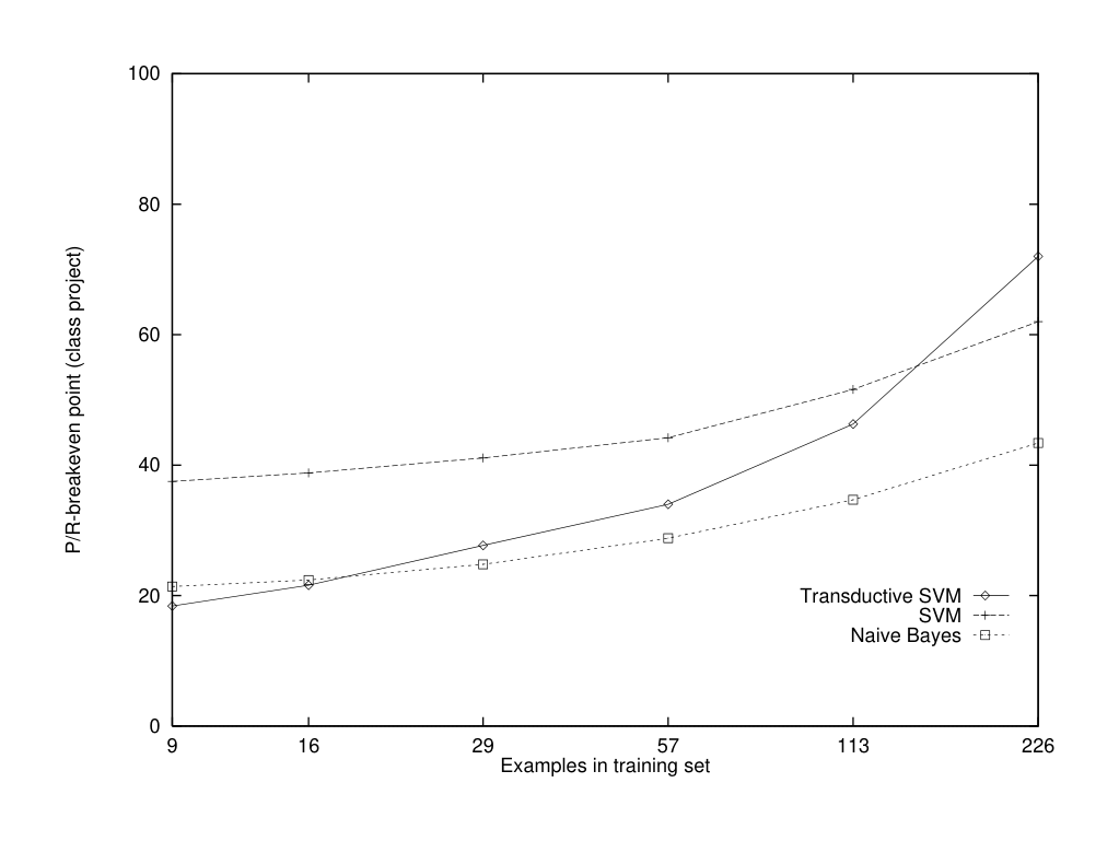
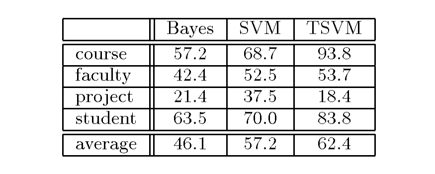
The results on the WebKB dataset are similar (figure 8). The average of the P/R-breakeven points increases from 57.2 to 62.4 by using the transductive approach. Nevertheless, for the category project the TSVM performs substantially worse, while the gain on the category course is large. Let's look at this in more detail. Figures 10 and 11 show how the performance changes with increasing training set size for course and project. While for course the TSVM nearly reaches its peak performance immediately, it needs more training examples to surpass the inductive SVM for project. Why does this happen?

{width=70%}

{width=80%}

First, project is the least populous class. Among 9 training examples, there is only one from the project category. But more importantly, a look at the project pages reveals that many of them give a description of the project topic. My conjecture is that the margin along this "topic dimension" is large, and so the TSVM tries to separate the test data by topic. Only when there are enough project pages with different topics in the training set, the generalization along the project topic is ruled out. Most course pages at Cornell, on the other hand, do not give much topic information besides the title, but rather link to assignments, lecture notes etc. So the TSVM is not "distracted" by large margins along the topics.

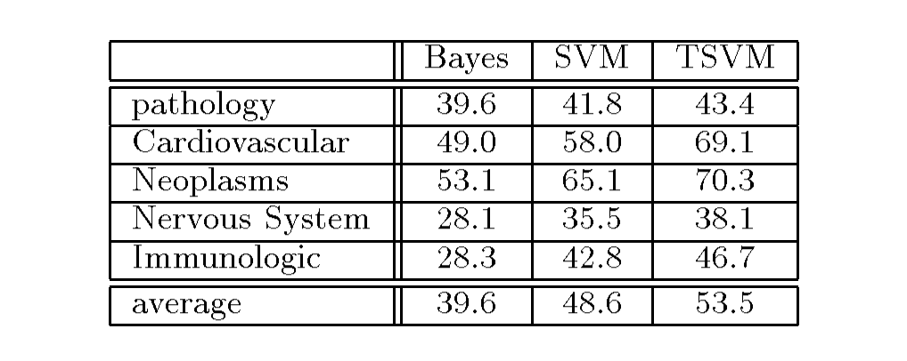
The results in figure 9 for the Ohsumed collection complete the empirical evidence given in this paper, also supporting its point.

6 Related Work

Section Summary: Earlier researchers explored ways to leverage unlabeled data for improving text classification. Nigam and colleagues applied the EM algorithm to a Naive Bayes model, yielding gains despite the model's unrealistic independence assumptions about words, while Blum and Mitchell introduced co-training, which boosts performance by exploiting multiple independent views of each example such as a web page and its incoming links. Separately, transductive methods were investigated as early as the 1970s, with later work showing modest accuracy improvements on benchmark datasets and techniques for estimating prediction confidence through algorithmic randomness.

Previously, Nigam et al. [Nigam et al., 1998] proposed another approach to using unlabeled data for text classification. They use a multinomial Naive Bayes classifier and incorporate unlabeled data using the EM-algorithm. One problem with using Naive Bayes is that its independence assumption is clearly violated for text. Nevertheless, using EM showed substantial improvements over the performance of a regular Naive Bayes classifier.

Blum and Mitchell's work on co-training [Blum and Mitchell, 1998] uses unlabeled data in a particular setting. They exploit the fact that, for some problems, each example can be described by multiple representations. WWW-pages, for example, can be represented as the text on the page and/or the anchor texts on the hyperlinks pointing to this page. Blum and Mitchell develop a boosting scheme which exploits a conditional independence between these representations.

Early empirical results using transduction can be found in [Vapnik and Sterin, 1977]. More recently, Bennett [Bennett, 1999] showed small improvements for some of the standard UCI datasets. For ease of computation, she conducted the experiments only for a linear-programming approach which minimizes the $L_1$ norm instead of $L_2$ and prohibits the use of kernels. Connecting to concepts of algorithmic randomness, [Gammerman et al., 1998] presented an approach to estimating the confidence of a prediction based on a transductive setting.

7 Conclusions and Outlook

Section Summary: The paper presented transductive support vector machines as a new approach to text classification, showing how margins can capture useful prior knowledge and how unlabeled test examples can improve learning when treated as part of the training process. It also described a practical training algorithm capable of handling large collections and reported consistent gains over standard methods, especially when labeled data are scarce. The section closes by outlining open theoretical and algorithmic questions, including better models of transductive generalization and whether the learned rule can be applied inductively to future examples.

This paper has introduced Transductive Support Vector Machines for text classification. Exploiting the particular statistical properties of text, it has identified that the margin of separating hyperplanes is a natural way to encode prior knowledge for learning text classifiers. By taking a transductive instead of an inductive approach, the test set can be used as an additional source of information about margins.

Introducing a new algorithm for training TSVMs that can handle 10,000 examples and more, this work presented empirical results on three test collections. On all data sets the transductive approach showed improvements over the currently best performing method, most substantially for small training samples and large test sets.

There are still a lot of open questions regarding transductive inference and SVMs. Particularly interesting is a PAC-style model for transductive inference to identify which concept classes benefit from transductive learning. How does the sample complexity behave for both the training and the test set? What is the relationship between the concept and the instance distribution? Regarding text classification in particular, is there a better basic representation for text, aligning margin and learning bias even better? Besides questions from learning theory, more research in algorithms for training TSVMs is needed. How well does the algorithm presented here approximate the global solution? Will the results get even better, if we invest more time into search? Finally, the transductive classification implicitly defines a decision rule. Is it possible to use this decision rule in an inductive fashion and will it perform well also on new test examples?

8 Acknowledgements

Section Summary: The authors thank Katharina Morik for her feedback on the paper and Tom Mitchell for helpful discussions during its development. They also credit Ken Lang for supplying portions of the code used in the project. The work was funded by a German research center focused on reducing complexity in data analysis.

Many thanks to Katharina Morik for comments on this paper and to Tom Mitchell for the discussion. Thanks also to Ken Lang for providing some of the code. This work was supported by the DFG Collaborative Research Center on Statistics "Complexity Reduction in Multivariate Data" (SFB475).

References

Section Summary: This section consists of a bibliography citing around twenty academic papers and books, mostly from the late 1990s, on machine learning techniques for text categorization and information retrieval. The references focus on support vector machines, semi-supervised approaches that combine labeled and unlabeled data, feature selection methods, and related statistical learning theory. They draw from conferences and journals such as ICML, ECML, COLT, and various AI venues, highlighting foundational contributions by researchers like Vapnik, Joachims, and Mitchell.

[Bennett, 1999] Bennett, K. (1999). Combining support vector and mathematical programming methods for classification. In Schölkopf, B., Burges, C., and Smola, A., editors, Advances in Kernel Methods - Support Vector Learning. MIT-Press.

[Blum and Mitchell, 1998] Blum, A. and Mitchell, T. (1998). Combining labeled and unlabeled data with co-training. In Annual Conference on Computational Learning Theory (COLT-98).

[Dumais et al., 1998] Dumais, S., Platt, J., Heckerman, D., and Sahami, M. (1998). Inductive learning algorithms and representations for text categorization. In Proceedings of ACM-CIKM98.

[Gammerman et al., 1998] Gammerman, A., Vapnik, V., and Vowk, V. (1998). Learning by transduction. In Conference on Uncertainty in Artificial Intelligence, pages 148–156.

[Joachims, 1997] Joachims, T. (1997). A probabilistic analysis of the Rocchio algorithm with TFIDF for text categorization. In Proceedings of International Conference on Machine Learning (ICML).

[Joachims, 1998] Joachims, T. (1998). Text categorization with support vector machines: Learning with many relevant features. In European Conference on Machine Learning (ECML).

[Joachims, 1999] Joachims, T. (1999). Making large-scale svm learning practical. In Schölkopf, B., Burges, C., and Smola, A., editors, Advances in Kernel Methods - Support Vector Learning. MIT-Press.

[McCallum and Nigam, 1998] McCallum, A. and Nigam, K. (1998). A comparison of event models for naive bayes text classification. In AAAI/ICML Workshop on Learning for Text Classification. AAAI Press.

[Mladenić, 1998] Mladenić, D. (1998). Feature subset selection in text learning. In European Conference on Machine Learning (ECML), Springer LNAI.

[Nigam et al., 1998] Nigam, K., McCallum, A., Thrun, S., and Mitchell, T. (1998). Learning to classify text from labeled and unlabeled documents. In Proceedings of the AAAI-98.

[Porter, 1980] Porter, M. (1980). An algorithm for suffix stripping. Program (Automated Library and Information Systems), 14(3):130–137.

[Raghavan et al., 1989] Raghavan, V., Bollmann, P., and Jung, G. (1989). A critical investigation of recall and precision as measures of retrieval system performance. ACM Transactions on Information Systems, 7(3):205–229.

[Salton and Buckley, 1988] Salton, G. and Buckley, C. (1988). Term weighting approaches in automatic text retrieval. Information Processing and Management, 24(5):513–523.

[van Rijsbergen, 1977] van Rijsbergen, C. (1977). A theoretical basis for the use of co-occurrence data in information retrieval. Journal of Documentation, 33(2):106–119.

[Vapnik, 1998] Vapnik, V. (1998). Statistical Learning Theory. Wiley.

[Vapnik and Sterin, 1977] Vapnik, V. and Sterin, A. (1977). On structural risk minimization or overall risk in a problem of pattern recognition. Automation and Remote Control, 10(3):1495–1503.

[Wapnik and Tscherwonenkis, 1979] Wapnik, W. and Tscherwonenkis, A. (1979). Theorie der Zeichenerkennung. Akademie Verlag, Berlin.

[Yang and Pedersen, 1997] Yang, Y. and Pedersen, J. (1997). A comparative study on feature selection in text categorization. In International Conference on Machine Learning (ICML).