📄 Executive Summary

Large-scale data analysis frequently relies on clustering to discover patterns, group similar items, and understand underlying data structures. Traditional K-means clustering is widely used for this purpose due to its simplicity, but it suffers from severe limitations: it is computationally slow on massive datasets, requires users to guess the correct number of clusters in advance, and often gets trapped in poor local solutions. Manually testing multiple cluster counts is computationally prohibitive and prone to error, especially when handling modern datasets containing hundreds of thousands of records.

The article develops and evaluates X-means, an exact clustering algorithm designed to automatically discover the optimal number of clusters within a specified range while dramatically accelerating computation. The objective is to eliminate the need for trial-and-error guessing and provide an efficient, statistically grounded method for large-scale clustering without resorting to data approximations.

The researchers evaluated X-means using both controlled synthetic datasets and real-world astronomical catalogs, including over 330,000 to 800,000 galaxy observations from the Sloan Digital Sky Survey and the Las Campanas Redshift Survey. The approach integrates a statistical scoring rule—the Bayesian Information Criterion—to evaluate local cluster splits, combined with an accelerated tree-based data structure that stores precomputed summary statistics to eliminate redundant geometric calculations.

The evaluation produced four key findings. First, X-means demonstrated substantial computational speed improvements, running twice as fast as an already accelerated K-means baseline and up to 32 times faster than standard K-means on large datasets. Second, the algorithm automatically identified the true number of clusters within approximately 15% on synthetic benchmarks while exhibiting lower distortion and higher statistical quality scores than standard approaches. Third, on astronomical data containing 330,000 galaxies, X-means finished in under 4 minutes, whereas standard K-means evaluating multiple cluster sizes required over 2 hours. Fourth, in large-scale sky surveys with 800,000 points, X-means completed clustering in 4.5 hours, whereas standard approaches failed to finish within allowable computational limits.

These findings indicate that organizations can perform robust, large-scale clustering in a fraction of the time previously required, eliminating the labor and operational risk associated with guessing cluster parameters. By replacing arbitrary user estimates with formal statistical model selection, the approach yields more reliable segmentations and lower distortion, reducing computational costs and enabling analysts to explore massive collections of low-dimensional spatial and metric data efficiently.

Organizations handling large spatial, scientific, or low-dimensional tabular datasets should adopt automated model selection methods like X-means when the true number of categories is unknown. Practitioners are advised to define reasonable minimum and maximum cluster bounds and deploy tree-accelerated implementations to maximize performance. Further engineering work is recommended to integrate alternate model scoring criteria and explore generalizations to probabilistic mixture models.

Confidence in these performance gains is high for datasets with low dimensionality, specifically up to four dimensions tested directly and up to seven dimensions based on foundational geometric methods. However, decision-makers should exercise caution when applying the method to very high-dimensional data, as the spatial tree structures become less efficient in higher-dimensional spaces unless combined with dimensionality-reduction techniques.

📚 What to read before this

No sufficiently relevant recommendations were found.

📚 What to read after this

No sufficiently relevant recommendations were found.

X-means: Extending $K$ -means with Efficient Estimation of the Number of Clusters

Dan Pelleg
[email protected]
Andrew Moore
[email protected]
School of Computer Science, Carnegie Mellon University, Pittsburgh, PA 15213 USA

Abstract

Despite its popularity for general clustering,

K

-means suffers three major shortcomings; it scales poorly computationally, the number of clusters

K

has to be supplied by the user, and the search is prone to local minima. We propose solutions for the first two problems, and a partial remedy for the third. Building on prior work for algorithmic acceleration that is not based on approximation, we introduce a new algorithm that efficiently searches the space of cluster locations and number of clusters to optimize the Bayesian Information Criterion (BIC) or the Akaike Information Criterion (AIC) measure. The innovations include two new ways of exploiting cached sufficient statistics and a new very efficient test that in one

K

-means sweep selects the most promising subset of classes for refinement. This gives rise to a fast, statistically founded algorithm that outputs both the number of classes and their parameters. Experiments show this technique reveals the true number of classes in the underlying distribution, and that it is much faster than repeatedly using accelerated

K

-means for different values of

K

1. Introduction

K

-means (Duda & Hart, 1973; Bishop, 1995) has long been the workhorse for metric data. Its attractiveness lies in its simplicity, and in its local-minimum convergence properties. It has, however, three main shortcomings. One, it is slow and scales poorly with respect to the time it takes to complete each iteration. Two, the number of clusters

K

has to be supplied by the user. Three, when confined to run with a fixed value of

K

it empirically finds worse local optima than when it can dynamically alter

K

. We offer solutions for these problems. Speed is greatly improved by embedding the dataset in a multiresolution

k d

-tree and storing sufficient statistics at its nodes. A careful analysis of the centroid locations allows for geometric “proofs” about the Voronoi boundaries, and (unlike all of (Deng & Moore, 1995; Zhang et al., 1995; Moore, 1999)) there is absolutely no approximation anywhere in the computation. An additional geometric computation, blacklisting, maintains a list of just those centroids that need to be considered for a given region (Pelleg & Moore, 2000). Blacklisting is not only extremely fast but also scales very well with the number of centroids, allowing tractable 10,000-means algorithms. This fast algorithm is used as a building-block in

X

-means: a new algorithm that quickly estimates

K

. It goes into action after each run of

K

-means, making local decisions about which subset of the current centroids should split themselves in order to better fit the data. The splitting decision is done by computing the Bayesian Information Criterion (BIC). We show how the blacklisting method naturally extends to ensure that obtaining the BIC values for all current centers and their tentative offspring costs no more than a single

K

-means iteration. We further enhance computation by caching stable-state information and eliminating the need to re-compute it.

We have experimented with

X

-means against a more traditional method that estimates the number of clusters by guessing

K

X

-means consistently produced better clustering on both synthetic and real-life data, with respect to BIC. It also runs much faster, even when the baseline is our accelerated blacklisting

K

-means.

2. Definitions

We first describe the naive

K

-means algorithm for producing a clustering of the points in the input into

K

clusters. It partitions the data-points into

K

subsets such that all points in a given subset “belong” to some center. The algorithm keeps track of the centroids of the subsets, and proceeds in iterations. Before the first iteration the centroids are initialized to random values. The algorithm terminates when the centroid locations stay fixed during an iteration. In each iteration, the following is performed:

For each point $x$ , find the centroid which is closest to $x$ . Associate $x$ with this centroid.
Re-estimate centroid locations by taking, for each centroid, the center of mass of points associated with it.

The

K

-means algorithm is known to converge to a local minimum of the distortion measure (that is, average squared distance from points to their class centroids). It is also known to be too slow for practical databases. Much of the related work does not attempt to confront the algorithmic issues directly. Instead, different methods of subsampling and approximation are proposed. A way to obtain a small “balanced” sample of points by sampling from the leaves of a

R *

tree is shown in Ester et al. (1995). Ng and Han (1994) suggested a simulated-annealing approach to direct the search in the space of possible partitions of the input points. Zhang et al. (1995) present a tree structure with sufficient statistics. It is used to identify outliers and speed computations. However, the calculated clusters are approximations, and depend on many parameters.

Note that although the starting centers can be selected arbitrarily,

K

-means is fully deterministic, given the starting centers. A bad choice of initial centers can have a great impact on both performance and distortion. Bradley and Fayyad (1998) discuss ways to refine the selection of starting centers through repeated subsampling and smoothing.

For the remainder of this paper we denote by

μj\mu_j

the coordinates of the

j

-th centroid. We will use the notation

(i)

to denote the index of the centroid which is closest to the

i

-th data-point. For example,

μ(i)\mu_{(i)}

is the centroid associated with the

i

-th point during an iteration.

D

is the input set of points, and

Di⊆DD_i \subseteq D

is the set of points that have

μi\mu_i

as their closest centroid. We let

R = ∣ D ∣

and

R_i = |D_i|

. The number of dimensions is

M

, and the Gaussian covariance matrix is

Σ=diag(σ2)\Sigma = \mathrm{diag}(\sigma^2)

3. Estimation of $K$

The algorithm as it was described up to this point can only be used to perform

K

-means where

K

is fixed and supplied by the user. We proceed now to demonstrate how to efficiently search for the best

K

. The framework now changes so the user only specifies a range in which the true

K

reasonably lies, and the output is not only the set of centroids, but also a value for

K

in this range which scores best by a model selection criterion such as BIC (see Section 3.2). We first describe the process conceptually, without paying much attention to the algorithmic details. Next, we derive the statistical tests used for scoring different structures. We then come back to the high-level description of the algorithm and show how it can be implemented efficiently using ideas deriving from blacklisting and the sufficient statistics stored in the

k d

-tree nodes.

3.1 Model Searching

In essence, the algorithm starts with

K

equal to the lower bound of the given range and continues to add centroids where they are needed until the upper bound is reached. During this process, the centroid set that achieves the best score is recorded, and this is the one that is finally output.

The algorithm consists of the following two operations repeated until completion.

X-means:

Improve-Params
Improve-Structure
If $K > K_{\max}$ stop and report the best-scoring model found during the search.

Else, Goto 1.

The Improve-Params operation is simple: it consists of running conventional

K

-means to convergence.

The Improve-Structure operation finds out if and where new centroids should appear. This is achieved by letting some centroids split in two. How can we decide what to split? We begin by describing and dismissing two obvious strategies, after which we will combine their strengths and avoid their weaknesses in our

X

-means strategy.

Splitting idea 1: One at a time. The first idea would be to pick one centroid, produce a new centroid nearby, run

K

-means to completion and see if the resulting model scores better. If it does, accept the new centroid. If it doesn’t, return to the previous structure. But this will need

O(K_{\max})

Improve-Structure steps until

X

-means is complete. And this begs the question of how to choose which centroid is most deserving to give birth.

And if it doesn’t improve the score what should be tried next? Perhaps all centroids could be tested in this way (and then we stick with the best) but since each test needs a run of

K

-means that would be an extremely expensive operation for adding only one centroid.

Splitting idea 2: Try half the centroids. The second idea is used in the SPLITLOOP system for Gaussian mixture model identification (Wasserman & Moore, in press). Simply choose (say) half the centroids according to some heuristic criterion for how promising they are to split. Split them, run

K

-means, and see if the resulting model scores better than the original. If so accept the split. This is a much more aggressive structure improvement, requiring only

O(\log K_{\max})

Improve-Structure steps until

X

-means completes. But what should the heuristic criterion be? Size of region owned by centroid? Distortion due to centroid? Furthermore, we will miss the chance to improve in cases when one or two centroids need to split but the rest do not.

Our solution achieves the benefits of ideas 1 and 2, but avoids the drawbacks and (as we will see in Section 3.3) can be turned into an extremely fast operation. We will explain by means of an example.

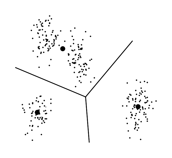
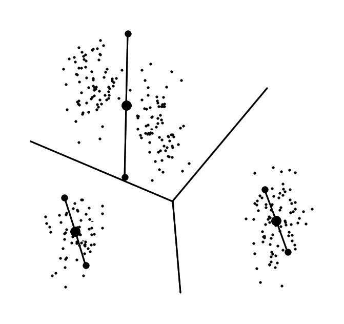
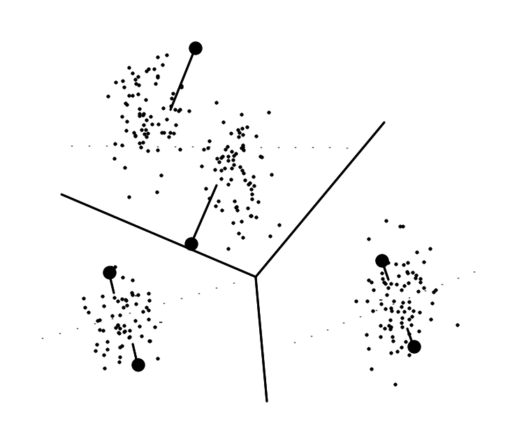
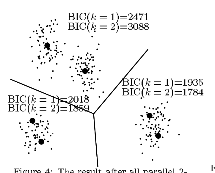
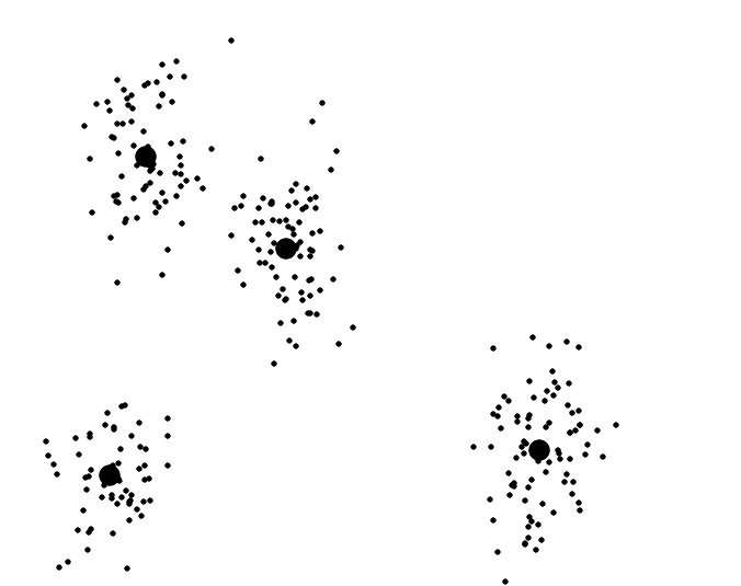
Figure 1 shows a stable

K

-means solution with 3 centroids. The boundaries of the regions owned by each centroid are also shown. The structure improvement operation begins by splitting each centroid into two children (Figure 2). They are moved a distance proportional to the size of the region in opposite directions along a randomly chosen vector. Next, in each parent region we run a local

K

-means (with

K = 2

) for each pair of children. It is local in that the children are fighting each other for the points in the parent’s region: no others. Figure 3 shows the first step of all three local 2-means runs. Figure 4 shows where all the children eventually end up after all local 2-means have terminated.

At this point a model selection test is performed on all pairs of children. In each case the test asks “is there evidence that the two children are modeling real structure here, or would the original parent model the distribution equally well”? The next section gives the details of one such test for

K

-means. According to the outcome of the test, either the parent or its offspring are killed. The hope is that centroids that already own a set of points which form a cluster in the true underlying distribution will not be modified by this process (that is, they will outlive their children). On the other hand, regions of the space which are not represented well by the current centroids will receive more attention by increasing the number of centroids in them. Figure 5 shows what happens after this test has been applied to the three pairs of children in Figure 4.

Therefore our search space covers all possible

2^K

post-splitting configurations, and it determines which one to explore by improving the BIC locally in each region. Compared with ideas 1 and 2 above, this allows an automatic choice of whether to increase the number of centroids by very few (in case the current number is very close to the true number) or very many (when the current model severely underestimates

K

). Empirically, we have also found that regional

K

-means runs with just 2 centers tend to be less sensitive to local minima.

We continue oscillating between Improve-Params and Improve-Structure until the upper bound for

K

is attained.

3.2 BIC Scoring

Assume we are given the data

D

and a family of alternative models

M_j

, where in our case different models correspond to solutions with different values of

K

How do we choose the best? We will use the posterior probabilities

Pr[Mj∣D]\mathrm{Pr}[M_j | D]

to score the models. In our case the models are all of the type assumed by

K

-means (that is, spherical Gaussians). To approximate the posteriors, up to normalization, we use the following formula from Kass and Wasserman (1995):

where

l^j(D)\hat{l}_j(D)

is the log-likelihood of the data according to the

j

-th model and taken at the maximum-likelihood point, and

p_j

is the number of parameters in

M_j

. This is also known as the Schwarz criterion.

The maximum likelihood estimate (MLE) for the variance, under the identical spherical Gaussian assumption, is:

The point probabilities are:

The log-likelihood of the data is

Fix

\leq n \leq K

. Focusing just on the set

D_n

of points which belong to centroid

n

and plugging in the maximum likelihood estimates yields:

The number of free parameters

p_j

is simply the sum of

K - 1

class probabilities,

\cdot K

centroid coordinates, and one variance estimate. To extend this formula for all centroids instead of one, we use the fact that the log-likelihood of the points that belong to all centroids in question is the sum of the log-likelihood of the individual centroids, and replace

R

above with the total number of points which belong to the centroids under consideration.

We use the BIC formula globally when

X

-means finally chooses the best model it encountered, and also locally in all the centroid split tests.

3.3 Acceleration

The

X

-means algorithm described so far can be implemented as is for small datasets. But so far we have neglected its most important feature. It was invented subject to the design constraint that it should be possible to use cached statistics to scale it up to datasets with massive numbers of records.

Accelerating

K

-means: We begin by concentrating on a single

K

-means iteration. The task is to determine, for every data-point, which centroid owns it. Then, we can compute the center-of-mass of all points which belong to a given centroid and that makes the new location for that centroid. Immediately we observe that showing that a subset of points all belong to a given centroid is just as informative as doing this for a single point, given that we have sufficient statistics for the subset (in our case the sufficient statistics are the number of points and their vector sum). Clearly it may save a lot of computation, provided that doing this is not significantly more expensive than demonstrating the ownership over a single point. Since the

k d

-tree imposes a hierarchical structure on the dataset, and we can easily compute sufficient statistics for its nodes at construction time, it makes a natural selection for the partition of the points. Each

k d

-node represents a subset of the data-set. It also has a bounding box, which is a minimal axis-parallel hyper-rectangle that includes all points in the subset. In addition it contains pointers to two children nodes, which represent a bisection of the points their parent owns.

Consider a set of counters, one for each centroid, which store a running total of the number of points that belong to each, as well as their vector sum. We now show how to update all the counters by scanning the

k d

-tree just once. The Update procedure is a recursive one, and accepts as parameters a node and a list of centroids that may own the points in it. Its task is to update the counters of the nodes in question with the appropriate values of the points in the node. The initial invocation is with the root node and the list of all centroids. After it returns the new locations may be calculated from the counters. The procedure considers the geometry of the bounding box and the current centroid locations to eliminate centroids from the list by proving they cannot possibly own any point in the current node. Hence the name “blacklisting”. Complete details, as well as proofs, can be found in Pelleg and Moore (2000). The point to remember here is that after shrinking the list, the procedure recurses on the children of the current node. The halting condition is when the list contains just one centroid; then, the centroid’s counters are incremented using the statistics stored in the

k d

-node. Frequently this happens in a shallow level of the

k d

-tree, and eliminates the work needed to traverse all of its descendants.

Accelerating Improve-Structure: The procedure described above works well to update the centroid locations of a global

K

-means iteration. We will now apply the same procedure to carry forward an Improve-Structure step. Recall that during Improve-Structure we perform 2-means in each Voronoi region of the current structure. We first make a list of the parent centroids, and use that as input to the Update procedure. The difference from the global iteration is in the action taken when the list reduces to a single centroid. This event signifies the fact that all points in the current node belong to the single centroid. All we have to do now is divide them between its children. To do this we simply make up a list containing just the two children, and recurse using this short list and the current node. The rest of the work is done by the Update procedure. After a full scan of the

k d

-tree has been carried out (possibly pruning away many nodes), the counters of the child centroids have their final values and their new locations can be computed. Now a new iteration can take place, and so on until the last of the centroid pairs has settled down.

Additional Acceleration: An interesting outcome of the local decision-making is that some regions of the space tend to become active (i.e., a lot of splitting and re-arrangement takes place) while other regions, where the centroids seem to have found the true classes, appear dormant. We can translate this pattern into further acceleration by using caching of statistics from previous iterations. Consider a

k d

-node that contains a boundary between two centroids (that is, either of the two centroids may own any of the node’s points). Although we must recurse down the tree in order to update the counters for the centers, there is no reason to do this again in the next iteration, provided that the centroids did not move, and that no other centroid has moved into a position such that it can own any of the node’s points. We therefore cache the contribution of this node to each of the centroids’ counters in the node, and subsequent iterations do not need to traverse the tree any further than the current node if the list of competing centroids matches.

To enable fast comparison of centroid locations against their position in previous iterations we employ a write-once data structure which does not permit alteration of centroid coordinates after the initial insertion. In case a centroid location changes, a new element has to be inserted and it is given a unique identifier. This way only a

O (1)

comparison of identifiers (per centroid) is needed. Clearly “old” centroids would never be accessed so there is no need to keep storing them in the data-structure. This allows for a fast and memory-efficient implementation using the original

\cdot K

memory plus a hash-table for identifier lookup. A further extension of this idea can also cache the children of a centroid in a regional iteration. Instead of being killed, they are moved to a “zombie” state and the next regional iteration resurrects them. Owing to the fact that their identifiers did not change, the caching mechanism immediately recalls the outcome of their last local iteration (which may have been reached after several re-positioning steps).

4. Experimental Results

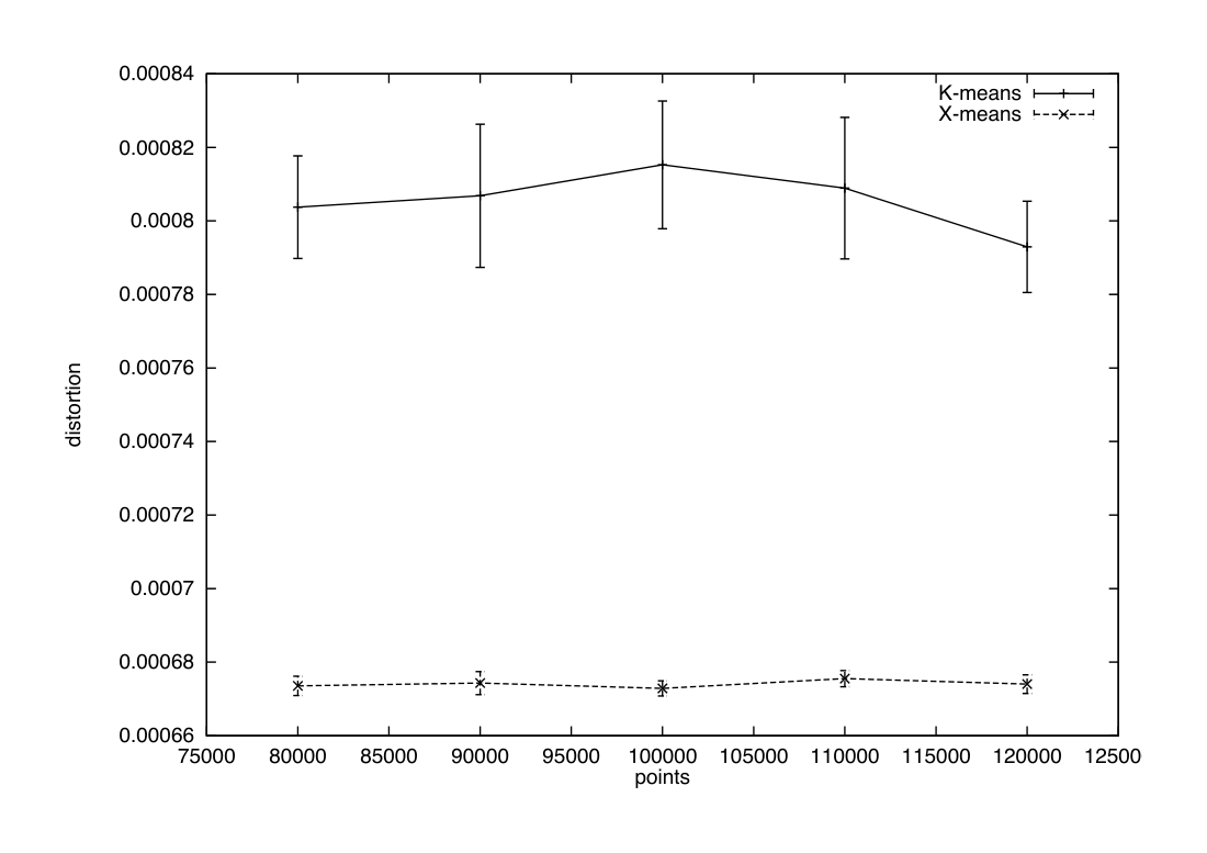
In our first experiment we tested the quality of the

X

-means solution against that of

K

-means. To define quality as the BIC value of the solution would be unfair to the

K

-means algorithm since it only tries to optimize the distortion (i.e., average squared distance from points to their centroids). We therefore compared both algorithms by the distortion of their output. Gaussian datasets were generated as in Pelleg and Moore (2000), then both algorithms were used. While

K

-means was given the true number of classes

K

, the

X

-means variant had to search for it in the range

\ldots K]

(see Figure 6). Interestingly, the distortion values for the

X

-means solutions are lower (meaning higher quality solutions). We may attribute this to the gradual way in which

X

-means adds new centroids in areas where they are needed. This contrasts with the once-only placement of initial centroids used by

K

-means.

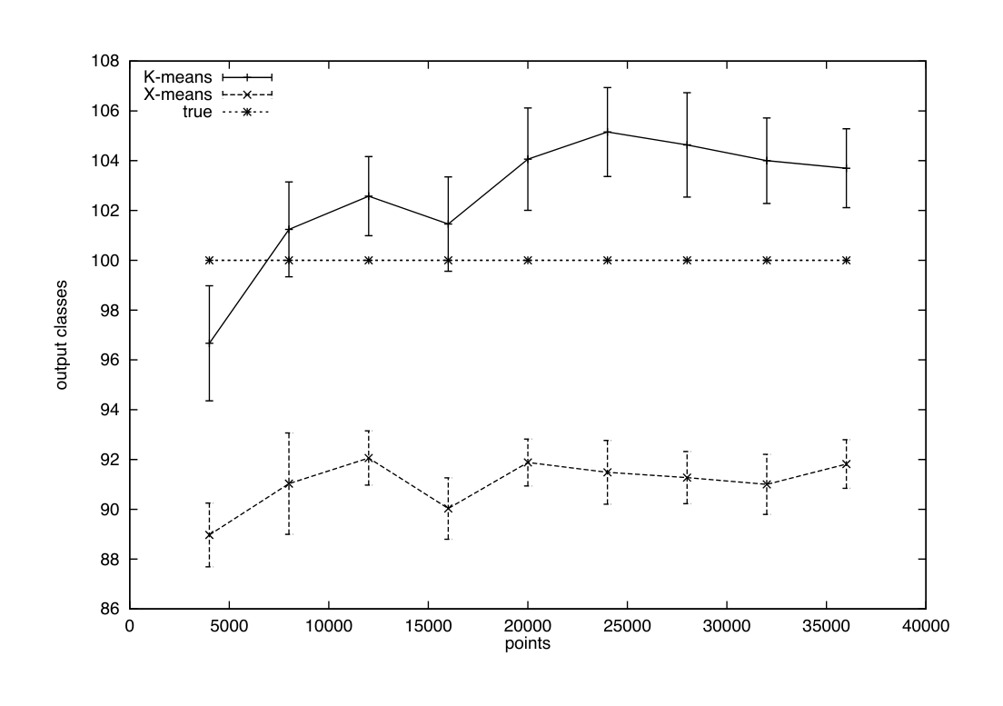
Another interesting question is how good

X

-means is at revealing the true number of classes. For comparison we used a variant of

K

-means which simply tries different values of

K

and reports the configuration which resulted in the best BIC. The permissible range for

X

-means was

\ldots 2K]

, and for

K

-means we used the 20 equally-distant values up to

2 K

. Averaged results are in Table 1 and detailed results for the 100-class case are in Figure 7. They show that

X

-means outputs a configuration which is within 15% from the true number of classes. We also see that

K

-means does better in this respect (about 6% average deviation). The results also show that

K

-means tends to over-estimate the number of classes, and also to output more classes as the number of records,

R

, increases, while

X

-means usually under-estimates the true

K

, and is in general insensitive to

R

Table 1: The mean absolute error vs. the number of classes output by the two algorithms, using 2-D data with 4000 to 36000 points.

classes	error
	$K$ -means	$X$ -means
50	$3.53 \pm 0.37$	$3.00 \pm 0.89$
100	$5.77 \pm 0.58$	$9.06 \pm 1.00$
150	$9.65 \pm 4.28$	$21.43 \pm 2.26$

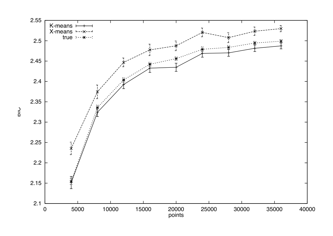
A slightly different picture arises when we examine the BIC score of the output configurations. Note that our

K

-means variant chooses the best configuration by its BIC score, so this is a fair comparison now. In Figure 8 we see that

X

-means scores not only better than

K

-means in this respect, but also outperforms the underlying distribution which was used to generate the data. This may be explained by random deviations in the data that cause it to be better modeled by fewer classes than there actually are. For example, two (or more) class centers, which are chosen at random, may fall extremely close to one another so they approximate a single class.

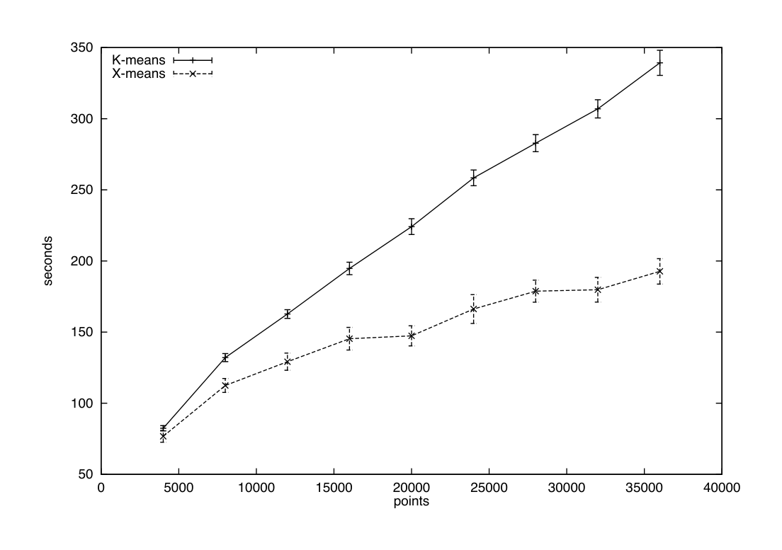
As far as speed is concerned,

X

-means scales much better than iterated

K

-means. As shown in Figure 9,

X

-means runs twice as fast for large problems. Note this is a competition against an already accelerated version of

K

-means as described in Pelleg and Moore (2000). When compared against naive

K

-means (that is, compute distances from every point to all centroids and pick the minimal),

X

-means fares much better. On a dataset of over 330,000 galaxies,

X

-means completed in 238 seconds where traditional

K

-means choosing among 10 values of

K

took 7793 seconds. Both algorithms were set up to perform just one iteration in the Improve-Params stage (and

X

-means is programmed to iterate once more in the Improve-Structure stage, and to augment the split by another global iteration). The quality of the

X

-means solution was superior in terms of both BIC and distortion.

An interesting application of

X

-means arises in the astrophysics domain. Given a dataset composed of galaxies and their

(x, y)

coordinates, one would like to ask what is a typical size of a cluster of galaxies. We selected the brightest galaxies in the The Sloan Digital Sky Survey (1998) data. This input set of approximately 800,000 sky objects¹ was divided by an

18 \times 3

grid (the ranges of the data are not proportional in both axis). The cells had approximately the same number of objects. On each cell with

R

objects we ran

K

-means iterated over the 10 values in the range

[R /1000, R /100]

and

X

-means searching for

K

in the same range, and recorded the resulting number of clusters (equivalently, the average cluster size).

As the survey progresses, we expect the number of galaxies to grow significantly.

The average cluster size according to

X

-means was

473 \pm 25.5

, and

572 \pm 40.8

according to

K

-means. While it is hard to validate these manually, we tend to believe

X

-means since it is free to choose the number of clusters from a wide range where

K

-means can only validate a small number of specified

K

. This fact is well reflected in the smaller variance of the

X

-means output. In early experiments, where the range for

K

was large and the number of sample points small, this effect was more noticeable (and indeed, in the early stages of a scientific research one’s guesses tend to be less educated, so we expect this to be a recurring theme).

In terms of run-time,

X

-means is not only faster, but increases its advantage as the number of points increases, similarly to the way it does so for synthetic datasets. An

X

-means run over the full dataset of some 800,000 points and 4,000 resulting centroids takes about 4.5 hours on a 600-Mhz DEC Alpha. A similar

K

-means invocation ran into a hard-coded limit after running for twice as long.

In a similar experiment on the important task of clustering galaxies in the Las Campanas Redshift Survey (1998) we compared

X

-means against a highly optimized but traditional (no kdtree) implementation of

K

-means. Traditional

K

-means tried 10 different values of

K

between 50 and 500. Both algorithms found solutions with almost identical BIC scores, though

X

-means chose a larger value of

K

X

-means completed its search eight times faster than

K

-means.

5. Conclusion

We have presented a new

K

-means based algorithm that incorporates model selection. By adopting and extending algorithmic improvements to

K

-means, it is efficient to the extent that running it once is cheaper than looping over

K

with the fixed-model algorithm. It uses statistically-based criteria to make local decisions that maximize the model’s posterior probabilities. Experimental results on both synthetic and real-life data show it is performing faster and better than

K

-means.

The choice of BIC as the splitting criterion is not the only possible one. While we have found BIC to perform well for our test-sets and applications, using other criteria, such as AIC or MDL, may make sense in other areas. Incorporating these measures into our algorithm is straightforward.

Another direct extension is the application of BIC (or similar criteria) to direct a model search in an unrestricted Gaussian EM algorithm (since blacklisting is assuming hard membership, this is non-trivial). Work in this vein is currently in progress (Wasserman & Moore). One can also think of other ways to conduct the search for a model, even under the

K

-means assumption (e.g., removing centroids, as well as adding them).

Using our fast algorithms, statistical analysis of millions of data-points and thousands of classes is performed in a matter of hours. Consequently, we are able to test astrophysical theories using observations that are much larger in scale than were ever available in the past. As hinted above, this work opens up an opportunity for a large class of algorithms to aid in such endeavors.

Finally, we need to consider the question of the dimensionality of the data. This paper has only empirically demonstrated

X

-means on up to four-dimensional data, although simpler algorithms (Pelleg & Moore, 2000) still give significant accelerations up to seven dimensions. But are even seven dimensions enough to be interesting? We say yes for two reasons.

First, many big-science disciplines need to cluster data-sets with between millions and billions of low-dimensional records very quickly. Spatial galaxy, color-space sky objects, and protein gel clustering are just three such examples on which we are collaborating with natural scientists.

Second, for high-dimensional data sets it is frequently preferable to model the PDF by a factored representation (Meila, 1999) such as a Bayesian network in which node distributions can be represented by lower-dimensional clusters.

X

-means is a step towards a fast inner-loop for these expensive algorithms.

Acknowledgements

We thank Larry Wasserman for invaluable help with the statistical foundations of this work. Support provided by an NSF KDI Award to Andrew Moore: DMS-9873442.

References

Bishop, C. M. (1995). Neural networks for pattern recognition. Oxford: Clarendon Press.

Bradley, P. S., & Fayyad, U. M. (1998). Refining initial points for K-Means clustering. Proceedings of the Fifteenth International Conference on Machine Learning (pp. 91–99). Morgan Kaufmann, San Francisco, CA.

Deng, K., & Moore, A. W. (1995). Multiresolution instance-based learning. Proceedings of the Twelfth International Joint Conference on Artificial Intelligence (pp. 1233–1239). San Francisco: Morgan Kaufmann.

Duda, R. O., & Hart, P. E. (1973). Pattern Classification and Scene Analysis. John Wiley & Sons.

Ester, M., Kriegel, H.-P., & Xu, X. (1995). A database interface for clustering in large spatial databases. Proceedings of First International Conference on Knowledge Discovery and Data Mining. Menlo Park: AAAI.

Kass, R., & Wasserman, L. (1995). A reference Bayesian test for nested hypotheses and its relationship to the Schwarz criterion. Journal of the American Statistical Association, 90, 773–795.

Las Campanas Redshift Survey (1998). http://manaslu.astro.utoronto.ca/~lin/lcrs.html.

Meila, M. (1999). Efficient Tree Learning. Doctoral dissertation, Massachusetts Institute of Technology, Department of Computer Science, Cambridge, MA.

Moore, A. W. (1999). Very fast mixture-model-based clustering using multiresolution kd-trees. Advances in Neural Information Processing Systems 10 (pp. 543–549). Morgan Kaufmann.

Ng, R. T., & Han, J. (1994). Efficient and effective clustering methods for spatial data mining. Proceedings of VLDB.

Pelleg, D., & Moore, A. (2000). Accelerating exact k-means with geometric reasoning (Technical Report CMU-CS-00-105). Carnegie Mellon University, Pittsburgh, PA. Also available from http://www.cs.cmu.edu/~dpelleg/.

The Sloan Digital Sky Survey (1998). www.sdss.org.

Wasserman, L., & Moore, A. Density Estimation with Accelerated, Exact, Mixture Models. In press.

Zhang, T., Ramakrishnan, R., & Livny, M. (1995). BIRCH: An efficient data clustering method for very large databases,. Proceedings of ACM SIGMOD (pp. 103–114).

X-means: Extending KKK-means with Efficient Estimation of the Number of Clusters

Abstract

1. Introduction

2. Definitions

3. Estimation of KKK

3.1 Model Searching

3.2 BIC Scoring

3.3 Acceleration

4. Experimental Results

5. Conclusion

Acknowledgements

References

X-means: Extending $K$ -means with Efficient Estimation of the Number of Clusters

3. Estimation of $K$