WhiteMatter: All-to-All Cross-Layer Connections via KV Mixing

Wenbo Zhang Xiang Ren
University of Southern California
wenboz,[email protected]

Abstract

In a Transformer, each layer attends to past tokens only through KV produced at its own depth, despite the presence of deeper representations during autoregressive decoding. Feedback architectures allow shallow consumer layers to attend to KV produced by deeper past-token representations, but give all consumer layers the same fixed connection patterns to source layers. We propose WhiteMatter, which connects every attention layer to the representations from all layers of each past token, with connection weights that can vary across consumer layers and adapt to the source token. For each token, a router implements these connections by mixing its $L$ layer states into $k$ KV channels that are cached for subsequent tokens; each consumer layer attends to one of the channels. The number of channels $k$ controls the KV-cache size. Setting $k<L$ reduces the cache's memory footprint. In our pretraining experiments, WhiteMatter outperforms a vanilla Transformer with $50%$ more layers and retains most of this gain with a $50%$ KV-cache compression.

Executive Summary: WhiteMatter introduces a new way for Transformer language models to connect layers across tokens during generation. Standard models restrict each layer to key-value (KV) states produced only at matching depths in past tokens. This wastes deeper representations already computed for those tokens and constrains how much information the model can use at each step. The restriction matters because it limits performance on language modeling while also forcing large KV caches that consume substantial memory during inference.

The work set out to test whether allowing every layer to draw flexibly from all past-layer representations—while controlling cache size—would improve modeling quality without changing decoding cost. Researchers implemented WhiteMatter by routing all layer states at each token into a smaller set of shared KV channels whose mixing weights adapt to the token content. Consumer layers then read from assigned channels. They trained 16-layer models from scratch on 8 billion tokens of FineWeb-Edu data and compared them against vanilla Transformers of 16, 24, and 32 layers plus a strong feedback baseline called LCKV.

Full-cache WhiteMatter cut held-out perplexity by 8.2 percent relative to the 16-layer vanilla model and slightly outperformed the 24-layer vanilla model. Halving the KV cache still yielded a 6.3 percent perplexity reduction versus the 16-layer baseline and remained within 1 percent of the 24-layer vanilla result, while beating the equal-cache LCKV variant by 5 percent. Both WhiteMatter configurations also improved downstream perplexity on LAMBADA and WikiText and raised accuracy on several multiple-choice tasks. Training and prefill required 2.3–3.3 times more compute than vanilla because of the iterative schedule needed to resolve feedback dependencies, yet decoding cost stayed essentially unchanged.

These results indicate that exposing shallow layers to deeper past representations can deliver meaningful quality gains at fixed depth or allow shallower models to match deeper ones while shrinking memory use. The gains hold even under substantial cache compression, which directly affects serving cost and context length. However, the higher training and prefill expense must be weighed against inference savings, and the experiments used only small models on a modest data budget.

Next steps should include scaling the approach to larger models and data volumes, testing more efficient fixed-point solvers to reduce iteration overhead, and running end-to-end latency benchmarks on optimized inference stacks. A separate prefill encoder could also be explored to decouple the cost of the first forward pass. The main limitations are the modest model size and token count used, plus the absence of production-scale decoding measurements; results should therefore be treated as indicative rather than definitive for frontier-scale deployment.

1. Introduction

Section Summary: Standard autoregressive Transformers generate hidden states layer by layer for each token, but each layer can only access matching-depth states from prior tokens, limiting how much past information the model can use. Prior approaches either add fixed feedback paths across tokens or cross-layer links within a token, yet none combine dynamic, per-layer selection of connections from all source depths. WhiteMatter solves this by routing all layers' states into a small set of content-dependent KV channels that different consumer layers can choose from, with an iterative schedule enabling efficient training and inference.

During decoding of an autoregressive Transformer ([1]), the model produces a stack of hidden states for a token before continuing to the next token. Each hidden state is generated at a corresponding layer and may contain unique information. However, when processing the next token, each layer can only attend to the KV produced from the hidden state at the same depth. Consequently, the model is unable to utilize all information it has already produced. In particular, the inaccessibility of past tokens' deeper states has been argued to limit computational depth and state tracking ([2]).

Two lines of work relax different parts of this restriction. Feedback architectures create a deep-to-shallow path across tokens. The Feedback Transformer ([3]) gives every consumer layer the same static connections to all layers' states at each past token. LCKV ([4]) instead uses the top-layer hidden state as KV source for all layers and introduces Jacobi iteration that makes training models with feedback connections tractable at scale. These architectures use the same source-layer connections for every consumer layer and input. Different consumer layers therefore cannot select different sources. A separate line provides feedforward cross-layer connections from earlier source layers to later consumer layers. DenseFormer ([5]), MUDDFormer ([6]), and related methods ([7, 8]) give different layers different connections to earlier-layer states within the current token. FusedKV ([9]) instead gives upper consumer layers static, layer-specific connections to KV produced by bottom and middle source layers of past tokens. These methods provide consumer-specific connectivity, and some are content-dependent. Their connections remain feedforward: a shallow current-token layer still cannot access deeper representations of past tokens.

The brain combines local computation with long-range communication. Gray matter contains neuronal cell bodies, while white matter contains nerve fibers that connect distant regions (Appendix A). These fibers form dense, often bidirectional connections between cortical areas ([10]). Each cortical area has a distinct pattern of connections, and activity along these pathways is dynamically modulated.

This organization motivates four architectural properties: direct connections between distant layers, deep-to-shallow feedback connections, consumer-specific connectivity, and dynamic modulation of connections. We propose WhiteMatter (Figure 1), which realizes all these properties through $k$ shared KV channels. At each token position, a router mixes the hidden states of all $L$ source layers into these channels. Each consumer layer selects one channel, so different consumers can receive different connections to source depths. Because the router reads the hidden states, the connection weights adapt to the source token.

Deep-to-shallow feedback is straightforward during autoregressive decoding, where past-token states are already final. During parallel training and prefill, however, each token's KV is built from its own completed hidden states, while those states depend in turn on earlier tokens' KV; a naive left-to-right resolution of this circular dependency would run sequentially in the sequence length. We resolve it by iteration with a cyclic Gauss–Seidel schedule that keeps the computation token-parallel.

We pretrained all models from scratch on $8$ B tokens of FineWeb-Edu with the same data, token budget, and optimizer settings. At $16$ layers and a full KV cache ($k{=}16$), WhiteMatter reaches $19.968$ held-out perplexity, which is $8.2%$ lower than the perplexity of a vanilla model ($21.747$) of the same depth and also slightly lower than that of a $24$-layer vanilla model ($20.181$). Halving the cache to $k{=}8$ gives $20.377$ perplexity, which is $5.0%$ below an LCKV baseline of the same cache size. Both configurations outperform all other 16-layer models on LAMBADA and WikiText. In a controlled model trained with exact autoregressive execution, cyclic Gauss–Seidel with $g{=}16$ comes within $1%$ of autoregressive perplexity in $4$ passes and makes converged prefill $13.9\times$ faster than exact autoregressive evaluation and $11.2\times$ faster than Jacobi iteration. For the $16$-layer experiments, cyclic training remains around $1.5\times$ more expensive than vanilla.

We summarize our contributions as follows: (1) WhiteMatter adds per-layer content-dependent connections to past representations from all source depths, implemented by producing KV from dynamic mixtures of all layers' states. (2) Sharing KV channels among consumer layers reduces the KV-cache size when $k<L$. (3) We apply a cyclic iteration schedule that improves training and prefill convergence speed and systematically explore the choice of iteration parameters. (4) Empirically, full-cache WhiteMatter lowers perplexity by $8.2%$ over the same-depth vanilla baseline and outperforms a $24$-layer model, while the half-cache configuration retains most of the gain with a $6.3%$ perplexity reduction.

2. Related Work

Section Summary: Researchers have explored feedback mechanisms that let shallower transformer layers draw on deeper representations from prior tokens, though most rely on fixed, shared, or single-source connection patterns that limit flexibility across layers and tokens. Other work mixes earlier-layer outputs directly in the residual stream via learned weights or attention, or shares key-value caches across layers to cut memory use, but these approaches typically cannot route deep past-token states to shallow consumers. A separate line of methods performs repeated computation on top-layer states or inserted latent positions to enable internal reasoning, at the cost of higher per-token computation that WhiteMatter avoids.

Deep-to-shallow feedback connections.

[3] replaces each layer's KV with a softmax-mixed pool over the $L$ layer states at each past token, shared across every consumer layer. [4] connects every consumer layer only to top-layer KV and contributes an iterative training procedure that makes such feedback architectures tractable at LLM scale. [11] propagates a single fixed deep source across tokens by injecting a cached middle-layer state into an earlier layer's residual stream. These three methods use either one connection pattern shared across consumers or a fixed connection from a single deep source. Recurrent Transformer ([12]) instead assigns each consumer its own layer's output as KV. None allows connections spanning all source layers to vary across consumer layers and adapt to each past token.

Feedforward cross-layer connections.

Within the residual stream, DenseFormer and LAuReL-PA replace the input to each layer with a mixture of earlier layers' outputs ([5, 13]). MUDDFormer makes the mixing weights content-dependent and computes separate aggregations for the Q, K, V, and residual streams ([6]). Hyper-Connections and mHC learn connections among multiple parallel residual streams ([7, 14]). DeepCrossAttention and Attention Residuals use input-dependent attention over earlier-layer outputs ([15, 8]), while Delta Attention Residuals attend over sublayer updates rather than cumulative states ([16]).

Related methods form connections through the key and value pathway. Value-residual methods add the first layer's value to later layers with per-layer coefficients or per-token gates ([17, 18]). Other methods share KV across layers using grouped patterns such as CLA, MLKV, and the YOCO cross-decoder ([19, 20, 21]); these are instances of the routing framework of [22]. FusedKV gives each upper layer a static mixture of KV from bottom and middle layers. Its Lite variant directly reuses middle-layer keys and bottom-layer values ([9]). [23] train with random cross-layer attention. These methods can reduce the KV cache size by sharing KV across layers, but the KV can only be produced by hidden states at the same layer or lower layers. They therefore do not expose deeper past-token representations to shallow consumer layers.

Latent reasoning via repeated computation.

Coconut ([24]) fine-tunes a language model to feed top-layer hidden states back as continuous latent inputs. The PonderLM family brings related repeated computation to pretraining by recycling input embeddings or inserting latent positions, with some variants using adaptive halting ([25, 26, 27, 28]). The inserted-position variants append latent inputs after selected observed tokens by feeding back those tokens' top-layer hidden states. Deep-to-shallow feedback therefore occurs only for tokens followed by a latent thought token. Another line reapplies a weight-tied layer stack for several recurrent steps per token ([29, 30, 31]). Unrolled, these models remain feedforward across depth, and attention reads same-depth states. Staircase attention ([32]) also recurs in time and generalizes the feedback memory of [3]. These approaches increase per-token computation with the recurrence count. WhiteMatter instead exposes all past-token states to every layer, uses no inserted positions, and has a decoding cost similar to that of a vanilla model.

3. Method

Section Summary: The method modifies a standard Transformer decoder by replacing each layer’s separate key-value projections with a shared cross-layer KV pool. At every token position a small router mixes the hidden states from all layers into a reduced set of k channels; these channels are projected once into keys and values, normalized, and stored, cutting the total KV cache to a fraction k/L of its usual size. During attention each layer simply reads its assigned channel from this compact cache according to a fixed cyclic rule, preserving normal autoregressive decoding.

We modify a Transformer decoder with $L$ layers and hidden width $D$. We write $T$ for sequence length, $i$ for a token position, $\ell$ for a layer index, and $j$ for a channel index. WhiteMatter retains the standard decoder blocks but replaces the $L$ per-layer KV projections with a cross-layer KV pool. At each past token, a data-dependent router mixes the hidden states of all $L$ layers into $k \le L$ shared channels. A set of $k$ shared projection pairs ${W^K_j, W^V_j}_{j=0}^{k-1}$ then converts these channels into keys and values. The overall KV cache is therefore $k/L$ of the size of a standard $L$-layer cache.

Each layer reads one channel using the fixed selection described in § 3.1. The key and value channels use separate signed mixtures, with weights $\alpha^K[i]$ and $\alpha^V[i]$ (§ 3.1). Our evaluated configurations learn $\alpha^K$ and $\alpha^V$ and use a fixed channel selection.

3.1 Cross-layer KV pool

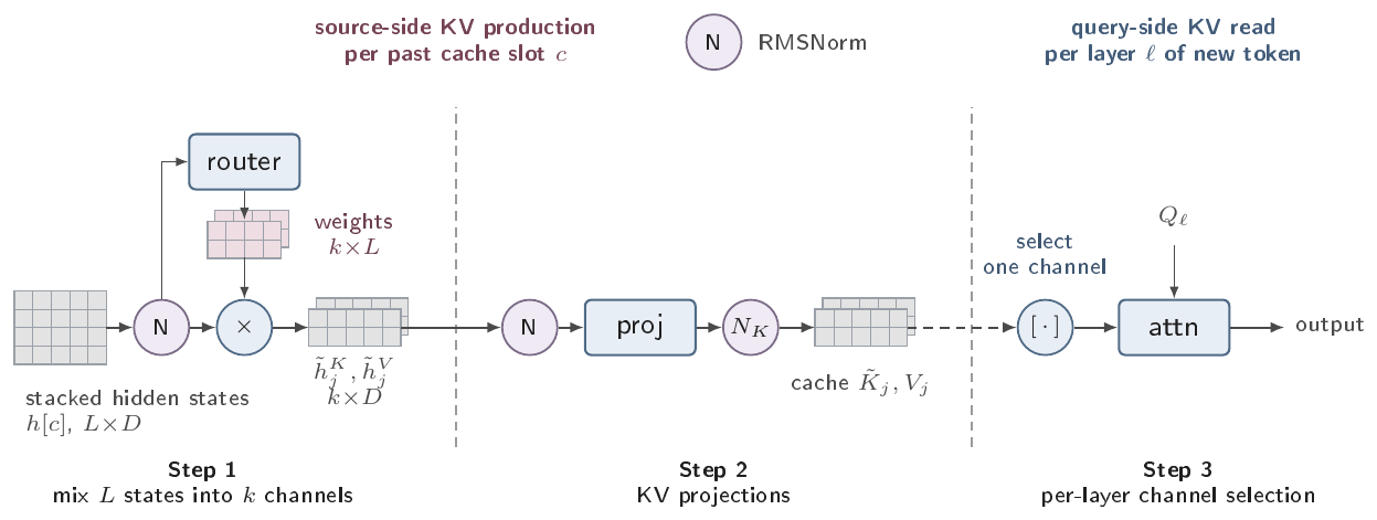
Step 1: mixing $L$ states into $k$ channels.

Let $h_\ell[i]\in\mathbb{R}^D$ be the hidden state entering layer $\ell$ at token $i$. At each position $i$, the pool combines the $L$ source states into $k$ channels using dynamic mixing weights, computed independently for the key and value branches. We describe the key branch; the value branch is identical with its own parameters.

Each source state is first RMS-normalized, giving $\hat{h}^K_\ell[i]$. This pre-mix norm puts the $L$ layers on a common scale and keeps their magnitudes from growing as they recur through the feedback loop.

The mixing weights $\alpha^K[i] \in \mathbb{R}^{k\times L}$ are produced by a linear router that reads the normed states. To reduce the router's size, it may read only every $p$ th source layer, counting down from layer $L{-}1$. This gives $L'=\lceil L/p\rceil$ router inputs while still producing mixing weights for all $L$ source layers. Stacking the selected states into $\xi^K[i] \in \mathbb{R}^{L'D}$,

$ \alpha^K[i] = \mathrm{reshape}\big(W^{\alpha K}, \xi^K[i] + b^{\alpha K}\big), \qquad W^{\alpha K}\in\mathbb{R}^{kL\times L'D}, \ \ b^{\alpha K}\in\mathbb{R}^{kL}, $

where the $kL$-dimensional output is reshaped to $k\times L$. Since $\alpha^K[i]$ depends on $\xi^K[i]$, the mixture is chosen anew at every position. Each channel is then the weighted sum

$ \tilde{h}^K_j[i] = \sum_{\ell=0}^{L-1} \alpha^K[i][j, \ell], \hat{h}^K_\ell[i]. $

The weights are signed and can therefore express differences among layer representations. The value branch uses the same construction with its own norm, router $W^{\alpha V}, b^{\alpha V}$, and weights $\alpha^V[i]$ applied to $\hat{h}^V_\ell[i]$.

Step 2: KV projections.

A second RMSNorm places the mixed channels at a common scale before they are projected into keys and values:

$ K_j[i] = W^K_j, \mathrm{RMSNorm}^K_j(\tilde{h}^K_j[i]), \qquad V_j[i] = W^V_j, \mathrm{RMSNorm}^V_j(\tilde{h}^V_j[i]), $

where $W^K_j, W^V_j\in\mathbb{R}^{H_{\mathrm{kv}}d\times D}$, $H_{\mathrm{kv}}$ is the number of KV heads, and $d$ is the head dimension. Per-channel key normalization and RoPE are applied before storage. Let $\mathrm{pos}(i)$ denote the rotary position assigned to token position $i$:

$ \tilde{K}_j[i] = \mathrm{RoPE}!\big(\mathrm{QKNorm}^K_j(K_j[i]);, \mathrm{pos}(i)\big). $

The cache stores the rotated, K-normalized key channel $\tilde{K}j[i]$ and the raw value channel $V_j[i]$ for $j = 0, \dots, k-1$, totaling $k \cdot T \cdot H{\mathrm{kv}} \cdot d$ elements for each of the key and value caches.

Step 3: per-layer channel selection.

When $k{=}1$, every layer reads the sole stored channel; when $k{=}L$, layer $\ell$ directly reads channel $\ell$. For $1<k<L$, we use a fixed cyclic selection, under which layer $\ell$ reads channel $\ell\bmod k$:

$ \hat{K}\ell[i] = \tilde{K}{\ell\bmod k}[i], \qquad \hat{V}\ell[i] = V{\ell\bmod k}[i], $

and attends with standard causal $\mathrm{SDPA}(Q_\ell, \hat{K}\ell, \hat{V}\ell)$. In the intermediate case, each channel is read by either $\lfloor L/k\rfloor$ or $\lceil L/k\rceil$ layers. A dense read over all channels would permit learned soft assignments, but would require each layer to stream all $k$ key and value channels from HBM. The fixed one-channel selection preserves one KV read per layer.

Router initialization.

We initialize the key and value routers with the same pattern. We set $W^{\alpha K}=W^{\alpha V}=0$, so the mixing weights initially depend only on the static biases and become content-dependent as the router weights are learned. We use three source-router bias initialization strategies. For $k{=}1$, the top initialization makes the single channel use the top-layer hidden state. For $1<k<L$, the cyclic initialization assigns source layer $\ell$ to channel $\ell\bmod k$, distributing interleaved source layers across channels. For $k=L$, the shifted-identity initialization assigns channel $j$ to source layer $\min(j+1, L-1)$, so each channel initially uses the next source layer, while the final channel remains assigned to the top layer.

3.2 Autoregressive decoding

At each autoregressive decoding step, the KV channels for all preceding tokens are already available in the cache. To process token $N$, we run the $L$ decoder layers using the existing cache and collect the hidden state entering each layer. After the final layer, we apply the cross-layer KV pool to these $L$ states and append the resulting channels to the cache. These channels are first read when processing token $N{+}1$. Thus, each decoding step consists of one layer-stack forward pass followed by one pool evaluation.

Because a token's KV channels are constructed only after its layer-stack forward pass, the token's queries must not read those channels. Standard causal attention would permit a query to read a KV entry at the same index. Masking the attention diagonal would prevent this but is incompatible with kernels such as FlashAttention-2 ([33]). We therefore prepend a learned dummy token to the KV cache, offsetting the cache by one position relative to the queries.

3.3 Parallel training and prefill

Efficient training and prefill rely on parallel computation across tokens, but processing each token requires KV channels derived from the completed hidden states of earlier tokens. The left-to-right procedure in § 3.2 resolves this dependency exactly but is sequential in $T$. We therefore formulate parallel execution as a fixed-point problem. The three schedules in Figure 3 target the same solution but differ in the degree of token-level parallelism and the number of passes required.

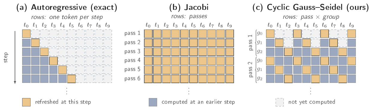
Jacobi iteration.

[4] proposed resolving the feedback dependency with Jacobi iteration. Let $H[i]={h_\ell[i]}_{\ell=0}^{L-1}$ denote the hidden states entering all layers at position $i$, and let $P[i]$ denote the corresponding key and value channels. Let $\mathrm{Pool}(H)$ apply the cross-layer pool independently at every position, and let $\mathrm{States}(X;P)$ apply the decoder blocks to all positions and return the per-layer hidden states, with each layer reading its fixed channel from $P$. For an input token sequence $X=(x[0], \dots, x[T{-}1])$, the cache channels $P$ and per-layer states $H$ at the exact solution satisfy

$ P = \mathrm{Pool}(H), \qquad H = \mathrm{States}(X;P). $

Jacobi iteration approximates this fixed point with $n$ token-parallel passes. We initialize $H^{(0)}$ by using each token's embedding as its state at every source layer. For $t=1, \dots, n$, we update

$ P^{(t)} = \mathrm{Pool}!\left(H^{(t-1)}\right), \qquad H^{(t)} = \mathrm{States}!\left(X;P^{(t)}\right). $

Thus, pass $t$ constructs the entire KV pool from the states produced by pass $t-1$, then updates all $T$ token positions in parallel. Information from the new states cannot affect the pool until the next pass, so multiple passes are required to approach the fixed point. Each pass evaluates the full $T\times L$ decoder computation; consequently, total cost grows linearly with the number of passes.

Cyclic Gauss–Seidel iteration.

We partition each pass into $g$ strided groups $\mathcal{G}_q={i:i\bmod g=q}$ and evaluate $\mathcal{G}0, \dots, \mathcal{G}{g-1}$ in order. Group $q$ reads the updated states of groups $0, \dots, q{-}1$ from the current pass and the previous-pass states of the rest. This is a block Gauss–Seidel update across groups and a parallel Jacobi update within each group. Each group contains $T/g$ positions distributed across the sequence and is updated in parallel, so an ordered sweep incorporates current-pass updates while retaining token-level parallelism for moderate $g$. The group count interpolates between the two schedules: $g{=}1$ is Jacobi iteration, and larger $g$ trades token-level parallelism for fewer passes, approaching sequential evaluation and becoming autoregressive at $g=T$. We use $g{=}8$.

Truncated backpropagation.

Backpropagating through many sequential passes would be computationally expensive. We follow [4] in carrying gradients only through the last $n_g \le n$ passes; earlier passes run under no_grad and serve to approach the fixed point.

4. Experiments

Section Summary: In the experiments section, researchers trained WhiteMatter language models from scratch on a large educational text dataset using the Qwen3 architecture and compared them against standard vanilla models of different depths as well as an LCKV baseline that shares key-value information across layers. At the same model depth and cache size, full-cache WhiteMatter reduced perplexity by over 8 percent relative to the vanilla baseline and even beat a deeper 24-layer vanilla model, while the half-cache version retained most of those gains and outperformed LCKV at equivalent cache sizes. Downstream evaluations on tasks such as LAMBADA, WikiText, and several multiple-choice benchmarks showed similar advantages for WhiteMatter, with three cyclic passes used during inference to maintain efficiency.

We evaluated whether WhiteMatter improves language modeling at fixed depth and cache size, whether the gains transfer to downstream tasks, and whether cyclic Gauss–Seidel reduces the cost of converged prefill.

4.1 Setup

Architecture.

All models used the Qwen3 decoder architecture ([34]), with hidden width $D{=}512$, intermediate size $1536$, and $6$ query and $3$ key/value heads of dimension $96$. Vanilla used this decoder unchanged. WhiteMatter replaced its $L$ per-layer KV projections with the cross-layer KV pool of § 3.1. We evaluated $L{=}16$ WhiteMatter models with $k{=}16$ (full cache) and $k{=}8$ (half cache).

Data.

We trained on the karpathy/fineweb-edu-100b-shuffle release of the FineWeb-Edu corpus ([35]), tokenized with the Qwen3-0.6B-Base tokenizer (vocabulary $151{,}936$) and packed to length $2048$ with an EOS separator. A document mask confined attention to each document. We reserved the final $5{,}000$ packed sequences of the shuffled corpus for testing; they were not used for training.

Optimization.

Every model was trained from scratch for $30{,}518$ steps ($8.0$ B tokens) at a global batch size of $128$. All evaluations used the final checkpoint. We optimized two-dimensional weight matrices with Muon ([36]) (momentum $0.95$, five Newton–Schulz steps) and the remaining parameters with AdamW ($\beta_1=0.9$, $\beta_2=0.95$). Both optimizers used a peak learning rate of $3{\times}10^{-4}$, $2%$ warmup, cosine decay to $10%$ of the peak, and weight decay of $0.1$. Training used bfloat16 autocast with fp32 master weights on eight NVIDIA RTX A6000 GPUs. Before DDP all-reduce, each GPU clipped the gradient norm at $1.0$.

WhiteMatter configuration.

We used $g{=}8$ groups with one no-gradient pass followed by two gradient-carrying passes. The key and value routers read every second source layer ($p=2$), and the two branches used the same initialization.

Baselines.

Alongside the $L{=}16$ vanilla model with a similar parameter count, we trained vanilla decoders at $L{=}24$ and $L{=}32$ using the same recipe, so depth was the only factor that changed. We also implemented the LCKV sandwich baseline ([4]) with $w\in{4, 7}$ warmup layers (vanilla layers that use their own hidden states to produce KV) split between the top and bottom; the condensed middle layers share one KV source. The $w{=}4$ configuration has two warmup layers at each boundary and $12$ condensed layers, yielding five unique KV sources ($5/16$ of the vanilla cache). The $w{=}7$ configuration has three bottom and four top warmup layers with nine condensed layers, yielding eight unique KV sources. It therefore has the same KV-cache size as half-cache WhiteMatter ($k{=}8$): $0.5\times$ that of vanilla. Following [4], both LCKV configurations used seven no-gradient Jacobi passes followed by two gradient-carrying passes. We trained them with the same data, token budget, and optimizer recipe as the other models.

4.2 Main results

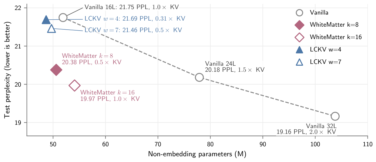
Figure 4 reports perplexity on the held-out test split ($5{,}000$ sequences, $10.2$ M tokens, length $2048$). At the same width and depth, full-cache WhiteMatter lowers perplexity from $21.747$ to $19.968$, an $8.2%$ relative reduction. It also outperforms the $24$-layer vanilla model, which reaches $20.181$ perplexity. Full-cache WhiteMatter and the $16$-layer vanilla baseline have $54.1$ M and $51.9$ M non-embedding parameters, respectively.

The half-cache WhiteMatter configuration reaches $20.377$ perplexity. It retains most of the full-cache improvement, lowering perplexity by $6.3%$ relative to the $16$-layer vanilla model and coming within $1.0%$ of the $24$-layer model. It has $50.6$ M non-embedding parameters, slightly fewer than the $16$-layer vanilla baseline.

LCKV $w{=}4$ reaches $21.692$ perplexity with $48.7$ M non-embedding parameters and $0.31\times$ the vanilla KV cache. Its perplexity is within $0.3%$ of the $16$-layer vanilla model. LCKV $w{=}7$ has $49.7$ M non-embedding parameters and reaches $21.461$ perplexity. WhiteMatter $k{=}8$, which has the same cache size, reaches $20.377$ perplexity, $5.0%$ lower than LCKV $w{=}7$.

4.3 Downstream evaluation

We evaluated the models with the lm-evaluation-harness in the zero-shot setting. WhiteMatter used three cyclic passes for every downstream task. Table 1 reports two language-modeling benchmarks and the multiple-choice tasks on which at least one model exceeds the random-choice baseline by two estimated standard errors, using normalized accuracy for the latter. Appendix C reports the complete suite and inclusion criterion.

\begin{tabular}{lrrrrrr}
  \hline
  Model & LAMBADA $\downarrow$ & WikiText $\downarrow$ &
  PIQA $\uparrow$ & HellaSwag $\uparrow$ & ARC-E $\uparrow$ &
  OBQA $\uparrow$ \\
  \hline
  Vanilla 16L & 127.47 & 49.34 & 60.88 & 31.67 & \textbf{47.39} & 29.00 \\
  LCKV $w{=}4$ & 107.52 & 48.81 & 62.57 & 32.52 & 45.66 & \textbf{31.20} \\
  LCKV $w{=}7$ & 102.97 & 49.02 & 62.24 & 32.40 & 46.21 & 30.00 \\
  WhiteMatter $k{=}8$ & 71.58 & 44.40 &
  62.35 & 33.61 & 45.71 & 29.60 \\
  WhiteMatter $k{=}16$ & \textbf{60.73} & \textbf{43.28} &
  \textbf{63.55} & \textbf{33.80} & 46.21 & 29.40 \\
  \hline
  Vanilla 24L & 97.40 & 44.71 & 62.73 & 33.21 & 47.94 & 31.80 \\
  Vanilla 32L & 79.39 & 41.44 & 63.82 & 34.35 & 47.90 & 32.20 \\
  \hline
  \end{tabular}

Among the $16$-layer models, full-cache WhiteMatter has the lowest perplexity on both language-modeling benchmarks and the highest accuracy on PIQA and HellaSwag. Both WhiteMatter variants outperform the $32$-layer vanilla model on LAMBADA ($60.73$ and $71.58$ vs. $79.39$ perplexity). Half-cache WhiteMatter outperforms equal-cache LCKV ($w{=}7$) on both language-modeling benchmarks and every reported multiple-choice task except ARC-Easy and OpenBookQA.

4.4 Prefill convergence and runtime

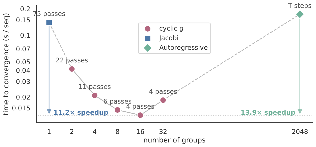
We isolated the schedule from training-time approximation using a separate $4$-layer model with $D{=}512$ and $k{=}4$, trained from scratch with exact autoregressive execution. Training used length $1024$, global batch size $96$, and $800$ steps ($78.6$ M tokens).[^1] We evaluated $192$ held-out length- $2048$ sequences; the exact autoregressive reference had perplexity $165.44$. For each group count $g$, we selected the smallest number of passes that yielded an average fp32 perplexity within $1%$ of the fp32 autoregressive reference. Timing was performed on one NVIDIA RTX A6000. Figure 5 reports time per sequence, computed by dividing batch execution time by $64$. Wall-clock measurements used compiled bfloat16 inference. We report the median time per sequence over $30$ trials after five warm-up trials ($10$ complete rollouts for autoregressive evaluation), excluding compilation.

[^1]: The model was small and lightly trained because exact autoregressive training is slow. Appendix B reports the same experiment on a larger model trained with cyclic iteration.

Jacobi ($g{=}1$) requires $75$ passes and takes $0.1393$ s/sequence. Autoregressive evaluation provides the reference in one serial left-to-right sweep and takes $0.1729$ s/sequence. Cyclic $g{=}16$ reaches the quality threshold in $4$ passes and takes $0.01245$ s/sequence, $11.2\times$ faster than Jacobi and $13.9\times$ faster than autoregressive evaluation. Increasing the group count further does not reduce the pass count: $g{=}32$ also requires $4$ passes but is slower because each pass costs more.

Jacobi iteration requires more than twice as many passes as cyclic $g{=}2$ to reach the quality threshold. This is unexpected because with twice as many passes, Jacobi performs the same number of sequential updates as cyclic $g{=}2$ and updates twice as many positions at each sequential step. We found that perplexity exhibits large oscillations across Jacobi iterations, whereas cyclic $g{=}2$ approaches the threshold more steadily. We have not identified the cause of this difference.

The LCKV baselines were trained and evaluated with nine Jacobi passes, far fewer than the $75$ needed for the controlled model to converge. However, they still attain lower held-out perplexity than the $16$-layer vanilla baseline. In § 5.1 we systematically explore the impact of training iteration schedules on model properties.

4.5 Compute cost

Table 2 reports measured per-token FLOPs for training, prefill, and decoding. The counts were produced by the PyTorch FLOP counter at sequence length $2048$ and validated against a closed-form derivation. LCKV used nine Jacobi iterations for both training and prefill. WhiteMatter used three cyclic iterations for training, two of which carried gradients, and three iterations for prefill, matching the downstream evaluation setting. We excluded the LM head from all FLOP measurements because its cost is disproportionately large for these small models, which use the Qwen3 tokenizer's large vocabulary.

\begin{tabular}{lrrrrrr}
  \hline
  Model & \multicolumn{2}{c}{Training} & \multicolumn{2}{c}{Prefill} & \multicolumn{2}{c}{Decode} \\
   {} & GFLOP/tok & $\times$ & GFLOP/tok & $\times$ & GFLOP/tok & $\times$ \\
  \hline
  Vanilla 16L & 0.444 & 1.00 & 0.142 & 1.00 & 0.179 & 1.00 \\
  Vanilla 24L & 0.665 & 1.50 & 0.212 & 1.50 & 0.269 & 1.50 \\
  Vanilla 32L & 0.887 & 2.00 & 0.283 & 2.00 & 0.359 & 2.00 \\
  LCKV $w{=}4$ & 1.421 & 3.20 & 0.935 & 6.61 & 0.173 & 0.97 \\
  LCKV $w{=}7$ & 1.174 & 2.65 & 0.738 & 5.21 & 0.175 & 0.97 \\
  WhiteMatter $k{=}8$ & 1.028 & 2.32 & 0.432 & 3.05 & 0.177 & 0.99 \\
  WhiteMatter $k{=}16$ & 1.111 & 2.50 & 0.467 & 3.30 & 0.184 & 1.03 \\
  \hline
  \end{tabular}

The decoding computation is nearly identical among all methods, with small differences due to the reduced KV projection cost and additional routing cost. WhiteMatter costs around $2.5\times$ the vanilla training FLOPs and $3.3\times$ the prefill FLOPs under the reported evaluation settings. The training multiplier is lower than the pass count because of truncated backpropagation. The LCKV warmup layers have no feedback connections, require no iteration, and cost the same as vanilla layers.

5. Analysis

Section Summary: Experiments on training schedules found that approaches closer to full convergence yielded better stability and lower perplexity, though they required more iterations at inference time, while shorter schedules sometimes hurt performance when the model was run beyond its training setup. Tests of KV cache sizes showed that even a single channel delivered a 16-fold compression along with a 7 percent perplexity improvement over a standard baseline, with further channels providing smaller additional gains. Ablation studies confirmed that both deep-to-shallow feedback across layers and dynamic routing were important, as removing either feature raised perplexity noticeably compared with the full approach.

Setup.

Unless stated otherwise, these experiments used the same $16$-layer, $D{=}512$ architecture, length- $2048$ FineWeb-Edu data, document masking, optimizer, and router parameterization as Section 4.1. We trained from scratch for $20{,}000$ optimizer steps at global batch size $8$ ($327.7$ M tokens) and evaluated the final checkpoint on the complete $5{,}000$-sequence test split.

5.1 Iteration schedules in training

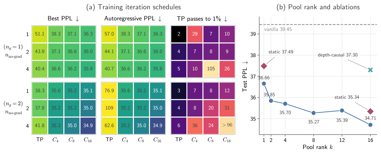
The main experiments showed that models trained with short iteration schedules could still outperform vanilla baselines. We next measured how the training schedule affects finite-pass and autoregressive quality and the number of inference iterations required for convergence (Figure 6 a).

We fixed $k{=}8$ and trained all combinations of $n_g\in{1, 2}$, $n_{\text{no-grad}}\in{1, 2, 4}$, and schedules ${\mathrm{TP}, C_4, C_8, C_{16}}$ with two random seeds. Here TP is full-sequence Jacobi iteration and $C_m$ is cyclic Gauss–Seidel with $m$ strided token groups. In every run the first $n_{\text{no-grad}}$ passes were detached and the final $n_g$ passes carried gradients. We evaluated three metrics for each checkpoint: (1) the best perplexity achieved at any pass count using the same schedule as training, (2) the perplexity that the model would achieve in autoregressive decoding, approximated by $32 $C_{16}$ $ passes, and (3) the number of token-parallel Jacobi passes required to reach within $ 1% of the best perplexity.

The results show three trends. First, the strongest evaluated schedule achieves $32%$ lower perplexity than the weakest schedule. Additional gradient or no-gradient passes and larger cyclic group counts improve performance with diminishing returns as the schedule approaches convergence. Second, models trained with schedules farther from the fixed point degrade when iterated beyond their training schedules, including under autoregressive decoding. Models trained with schedules closer to the fixed point remain stable after convergence. Third, the latter models require more inference iterations to converge. For a common measure of convergence difficulty, we computed this pass count with Jacobi iteration for every training schedule. Cyclic evaluation required fewer passes in practice.

5.2 KV cache compression

We fixed the iteration schedule ($n_{\text{no-grad}}{=}1$, $n_g{=}2$, $C_8$), then trained models with $k\in{1, 2, 4, 8, 12, 16}$. Figure 6 b shows the results. The dashed baseline is a vanilla model trained under the same conditions. Overall, more channels improve performance with diminishing returns. Even a single channel ($k{=}1$) outperforms the vanilla baseline, with a $16\times$ KV-cache compression and a $7.3%$ perplexity reduction.

5.3 Ablation studies

We performed two ablation experiments. Figure 6 b shows both results.

Deep-to-shallow feedback.

We trained a model with KV mixing but no deep-to-shallow feedback. At layer $\ell$, KV is formed only from hidden states at layers $0, \ldots, \ell$. Consequently, this model does not require iteration and has training and prefill costs similar to those of vanilla. Its KV-cache size matches those of full-cache WhiteMatter ($k{=}16$) and vanilla. The model outperforms vanilla due to dynamic KV mixing, but its perplexity remains $7.5%$ higher than that of full-cache WhiteMatter. It also underperforms the $k{=}1$ model despite using a $16\times$ larger KV cache. These results show that deep-to-shallow feedback is a key component of WhiteMatter.

Dynamic routing.

We trained two models with static learnable mixing weights and no dynamic router, one with $k{=}16$ and one with $k{=}1$. Both static models have about $2%$ higher perplexity than their dynamically routed counterparts.

Limitations

Section Summary: WhiteMatter achieves faster decoding and lower memory use during inference but incurs substantially higher computational costs during training and the initial prefill stage, requiring roughly two to three times the floating-point operations of standard methods. The reported results come only from small models trained on a limited data budget, so it remains unclear how the approach scales in quality or efficiency to larger models and datasets. The work also lacks optimized end-to-end decoding benchmarks, leaving those evaluations for future study.

Training and prefill costs.

WhiteMatter targets decode-time performance and KV-cache efficiency at the cost of iterative training and prefill. Although decoding uses similar FLOPs to vanilla decoding and can reduce memory consumption, training and prefill require either autoregressive processing or multiple parallel iterations. Cyclic Gauss–Seidel converges in fewer passes than Jacobi iteration, but WhiteMatter training and three-pass prefill still require $2.3$ – $2.5\times$ and $3.1$ – $3.3\times$ the vanilla FLOPs, respectively. More efficient fixed-point solvers or a separate prefill encoder could reduce these costs.

Empirical scope.

Our main results are based on small models trained with an $8$ B-token budget. These experiments therefore do not establish how the quality or systems trade-offs scale with model size and data. We report cache size and schedule convergence, but do not provide an optimized end-to-end decoding benchmark. Evaluating larger models and optimized end-to-end decoding remains future work.

Appendix

Section Summary: The appendix presents supplementary visualizations and data from a study on AI language models. It includes brain imaging figures showing white-matter connections reconstructed from MRI scans, along with performance details for a larger model variant demonstrating faster convergence using a specialized cyclic training approach compared to standard methods. It also provides complete benchmark results across numerous language understanding tasks, noting which evaluations were highlighted or excluded based on how models performed relative to chance levels.

A. White-matter connectivity

:::: cols="2"

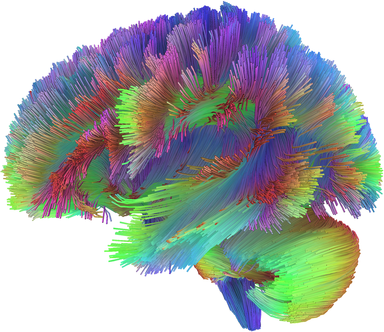
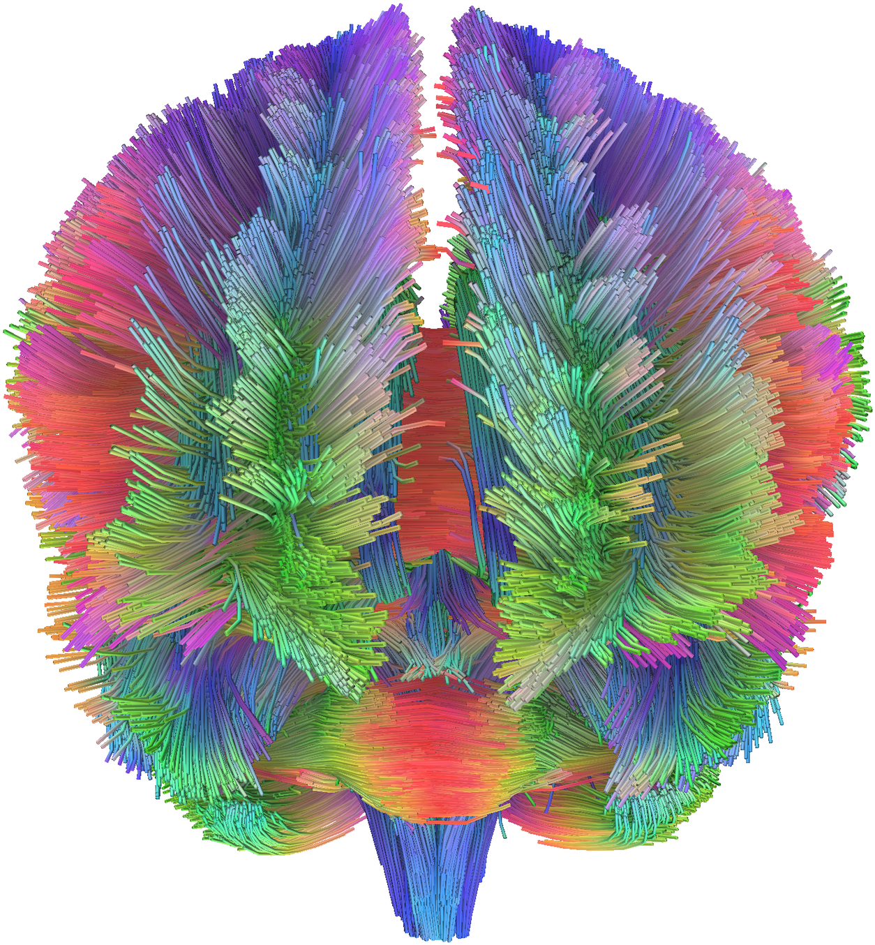
Figure 7: Whole-brain white-matter tractography. A population-averaged human structural connectome reconstructed from diffusion MRI, rendered as fiber tracts in sagittal (left) and coronal (right) views. The tracts span the brain and arc between distant regions in every direction; color encodes local fiber orientation (red: left–right, green: anterior–posterior, blue: superior–inferior). Rendered with DSI Studio ([37]) from its population-averaged human template ([38]), built from Human Connectome Project data ([39]). ::::

B. Convergence of a larger cyclic-trained model

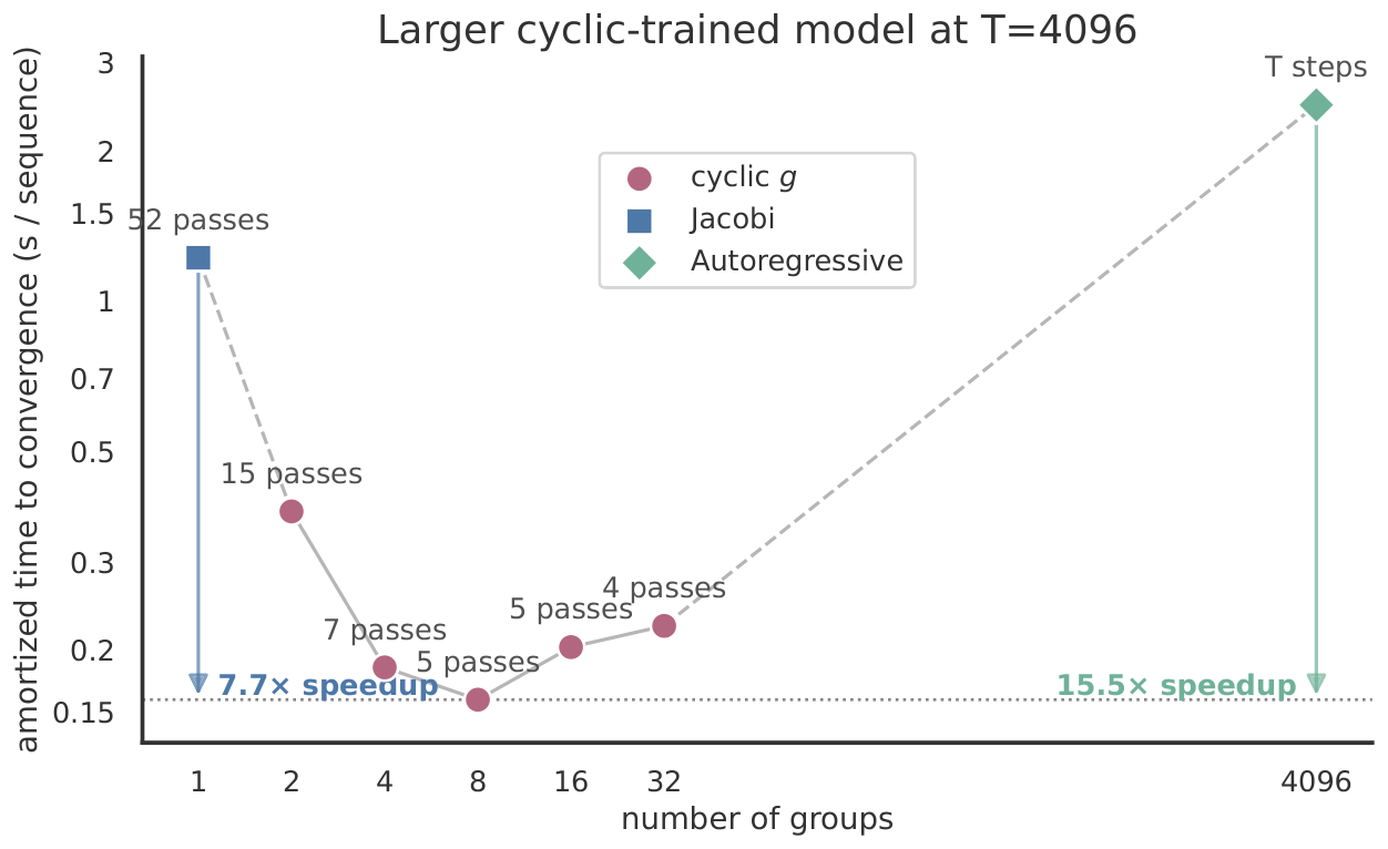
The model in Figure 8 was trained for $122{,}000$ steps at global batch size $8$ and length $4096$ (approximately $4.0$ B tokens) using a cyclic $g{=}8$ schedule. Pass counts used fp32 average perplexity over the same number of held-out sequences as the main experiment ($192$), with convergence defined as coming within $1%$ of the fp32 autoregressive reference. Timing used compiled bfloat16 execution, a fixed physical batch of $64$ on an NVIDIA RTX A6000, five warm-up trials and $30$ measured trials ($10$ complete autoregressive rollouts).

Jacobi requires $52$ passes and takes $1.220$ s/sequence. Cyclic $g{=}8$ requires $5$ passes and takes $0.159$ s/sequence, $7.7\times$ faster than Jacobi and $15.5\times$ faster than the $2.470$ s/sequence autoregressive rollout.

C. Full downstream results

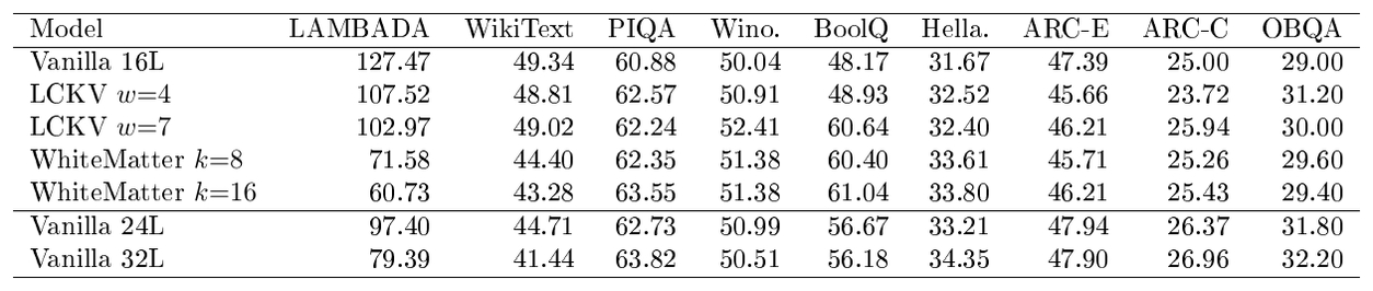
Table 3 reports every task in the zero-shot lm-evaluation-harness suite. PIQA, HellaSwag, ARC-Easy, ARC-Challenge, and OpenBookQA use normalized accuracy; WinoGrande and BoolQ use accuracy. The main table includes a multiple-choice task when at least one model exceeds the random-choice baseline by two estimated standard errors; for BoolQ we use the majority-class baseline of $62.17%$. WinoGrande remains near its $50%$ random-choice baseline, ARC-Challenge remains near its $25%$ random-choice baseline, and all models remain below the BoolQ baseline. We therefore omit these three columns from the main-text table.

::: {caption="Table 3: Complete zero-shot downstream results. LAMBADA and WikiText report perplexity; all other columns report accuracy in percent."}

:::

References

Section Summary: This section consists of a numbered bibliography with over thirty academic citations, primarily recent conference papers, preprints, and journal articles focused on transformer models and their architectural variants. The entries cover foundational work on attention mechanisms alongside newer research exploring efficiency improvements, residual connections, memory caching, and recurrent or layered processing in neural networks. Each reference includes authors, publication details, titles, and links to sources like arXiv or conference proceedings.

[1] Ashish Vaswani et al. (2017). Attention Is All You Need. In Advances in Neural Information Processing Systems. https://proceedings.neurips.cc/paper/7181-attention-is-all-you-need.

[2] Michael C. Mozer et al. (2026). The Topological Trouble With Transformers. arXiv preprint arXiv:2604.17121.

[3] Angela Fan et al. (2021). Addressing Some Limitations of Transformers with Feedback Memory. In International Conference on Learning Representations. https://openreview.net/forum?id=OCm0rwa1lx1.

[4] Haoyi Wu and Kewei Tu (2024). Layer-Condensed KV Cache for Efficient Inference of Large Language Models. In Proceedings of the 62nd Annual Meeting of the Association for Computational Linguistics (Volume 1: Long Papers). https://arxiv.org/abs/2405.10637.

[5] Matteo Pagliardini et al. (2024). DenseFormer: Enhancing Information Flow in Transformers via Depth Weighted Averaging. In International Conference on Machine Learning (ICML). https://arxiv.org/abs/2402.02622.

[6] Da Xiao et al. (2025). MUDDFormer: Breaking Residual Bottlenecks in Transformers via Multiway Dynamic Dense Connections. In Proceedings of the 42nd International Conference on Machine Learning. pp. 68440–68458. https://proceedings.mlr.press/v267/xiao25d.html.

[7] Defa Zhu et al. (2025). Hyper-Connections. In International Conference on Learning Representations. https://openreview.net/forum?id=9FqARW7dwB.

[8] Kimi Team (2026). Attention Residuals. arXiv preprint arXiv:2603.15031.

[9] Hongzhan Lin et al. (2026). Reconstructing KV Caches with Cross-layer Fusion For Enhanced Transformers. In International Conference on Learning Representations (ICLR). https://arxiv.org/abs/2512.03870.

[10] Nikola T. Markov et al. (2014). A weighted and directed interareal connectivity matrix for the macaque cerebral cortex. Cerebral Cortex. 24(1). pp. 17–36. doi:10.1093/cercor/bhs270.

[11] Ziyang Cai et al. (2026). T$^2$MLR: Transformer with Temporal Middle-Layer Recurrence. arXiv preprint arXiv:2607.15178.

[12] Costin-Andrei Oncescu et al. (2026). The Recurrent Transformer: Greater Effective Depth and Efficient Decoding. arXiv preprint arXiv:2604.21215.

[13] Gaurav Menghani et al. (2025). LAuReL: Learned Augmented Residual Layer. In Proceedings of the 42nd International Conference on Machine Learning. pp. 43826–43836. https://proceedings.mlr.press/v267/menghani25a.html.

[14] Zhenda Xie et al. (2025). mHC: Manifold-Constrained Hyper-Connections. arXiv preprint arXiv:2512.24880.

[15] Mike Heddes et al. (2025). DeepCrossAttention: Supercharging Transformer Residual Connections. arXiv preprint arXiv:2502.06785.

[16] Cheng Luo et al. (2026). Delta Attention Residuals. arXiv preprint arXiv:2605.18855.

[17] Zhanchao Zhou et al. (2024). Value Residual Learning. arXiv preprint arXiv:2410.17897.

[18] Skye Gunasekaran et al. (2026). Transformers with Selective Access to Early Representations. arXiv preprint arXiv:2605.03953.

[19] William Brandon et al. (2024). Reducing Transformer Key-Value Cache Size with Cross-Layer Attention. arXiv preprint arXiv:2405.12981.

[20] Zayd Muhammad Kawakibi Zuhri et al. (2024). MLKV: Multi-Layer Key-Value Heads for Memory Efficient Transformer Decoding. arXiv preprint arXiv:2406.09297.

[21] Yutao Sun et al. (2024). You Only Cache Once: Decoder-Decoder Architectures for Language Models. arXiv preprint arXiv:2405.05254.

[22] You Wu et al. (2025). A Systematic Study of Cross-Layer KV Sharing for Efficient LLM Inference. In Proceedings of the 2025 Conference of the Nations of the Americas Chapter of the Association for Computational Linguistics: Human Language Technologies (Volume 2: Short Papers). pp. 396–403. doi:10.18653/v1/2025.naacl-short.34. https://aclanthology.org/2025.naacl-short.34/.

[23] Anastasiia Filippova et al. (2026). Stochastic KV Routing: Enabling Adaptive Depth-Wise Cache Sharing. arXiv preprint arXiv:2604.22782.

[24] Shibo Hao et al. (2025). Training Large Language Models to Reason in a Continuous Latent Space. In Conference on Language Modeling. https://arxiv.org/abs/2412.06769.

[25] Boyi Zeng et al. (2026). PonderLM: Pretraining Language Models to Ponder in Continuous Space. In International Conference on Learning Representations. https://openreview.net/forum?id=UrM4MNRYZm.

[26] Shixiang Song et al. (2026). AdaPonderLM: Gated Pondering Language Models with Token-Wise Adaptive Depth. arXiv preprint arXiv:2603.01914.

[27] Boyi Zeng et al. (2025). PonderLM-2: Pretraining LLM with Latent Thoughts in Continuous Space. arXiv preprint arXiv:2509.23184.

[28] He Li et al. (2026). PonderLM-3: Adaptive Token-Wise Pondering with Differentiable Masking. arXiv preprint arXiv:2603.02023.

[29] Mostafa Dehghani et al. (2019). Universal Transformers. In International Conference on Learning Representations (ICLR). https://arxiv.org/abs/1807.03819.

[30] Jonas Geiping et al. (2025). Scaling up Test-Time Compute with Latent Reasoning: A Recurrent Depth Approach. arXiv preprint arXiv:2502.05171.

[31] Rui-Jie Zhu et al. (2025). Scaling Latent Reasoning via Looped Language Models. arXiv preprint arXiv:2510.25741.

[32] Da Ju et al. (2022). Staircase Attention for Recurrent Processing of Sequences. In Advances in Neural Information Processing Systems. https://openreview.net/forum?id=NiCJDYpKaBj.

[33] Tri Dao (2024). FlashAttention-2: Faster Attention with Better Parallelism and Work Partitioning. In International Conference on Learning Representations (ICLR). https://arxiv.org/abs/2307.08691.

[34] An Yang et al. (2025). Qwen3 Technical Report. arXiv preprint arXiv:2505.09388.

[35] Guilherme Penedo et al. (2024). The FineWeb Datasets: Decanting the Web for the Finest Text Data at Scale. In Advances in Neural Information Processing Systems (NeurIPS) Datasets and Benchmarks Track. https://arxiv.org/abs/2406.17557.

[36] Keller Jordan et al. (2024). Muon: An Optimizer for Hidden Layers in Neural Networks. https://kellerjordan.github.io/posts/muon/.

[37] Fang-Cheng Yeh (2025). DSI Studio: An Integrated Tractography Platform and Fiber Data Hub for Accelerating Brain Research. Nature Methods. 22. pp. 1617–1619. doi:10.1038/s41592-025-02762-8.

[38] Fang-Cheng Yeh et al. (2018). Population-averaged atlas of the macroscale human structural connectome and its network topology. NeuroImage. 178. pp. 57–68. doi:10.1016/j.neuroimage.2018.05.027.

[39] David C. Van Essen et al. (2013). The WU-Minn Human Connectome Project: An overview. NeuroImage. 80. pp. 62–79. doi:10.1016/j.neuroimage.2013.05.041.