Do Differentiable Simulators Give Better Policy Gradients?

Hyung Ju Terry SuhMax SimchowitzKaiqing ZhangRuss Tedrake

article2022ICML154 citationsOutstanding Paper 2022

Explains why physical discontinuities and stiffness introduce severe bias and variance into differentiable simulator gradients, while developing a hybrid alpha-order estimator that effectively blends zeroth- and first-order techniques for reliable policy optimization.

Listen

Modern robotics and continuous control increasingly rely on simulation to train policies via reinforcement learning. While differentiable simulators promise substantially faster computation by providing exact first-order derivatives, it has remained unclear whether these exact gradients actually improve optimization in complex physical tasks involving contact, friction, and stiff dynamics.

The article systematically evaluates the trade-offs between first-order gradient estimators (which leverage exact simulator derivatives) and zeroth-order estimators (which rely on function evaluations under randomized smoothing). To solve the pitfalls of both extremes, the article proposes and demonstrates an adaptive interpolation method called the alpha-order gradient estimator.

The evaluation combines mathematical analysis of bias and variance with simulated robotic benchmarks, including object pushing under varying spring stiffness, sliding trajectories governed by Coulomb friction, double-pendulum chaotic dynamics, and a paddle tennis policy optimization task. These experiments compare optimization stability, trajectory quality, and convergence speed across the different gradient estimators.

The investigation reveals four primary findings. First, first-order estimators become severely biased in the presence of physical discontinuities—such as collisions or geometric boundaries—causing optimization to stall in flat regions or fail entirely. Second, continuous approximations of contact do not eliminate this problem; under finite sample sizes, stiff continuous relaxations exhibit "empirical bias," appearing to have near-zero variance while producing entirely incorrect gradient directions. Third, in stiff contact regimes or chaotic dynamics, the variance of first-order estimators escalates dramatically over long horizons, whereas zeroth-order estimators remain unbiased and often exhibit lower variance. Fourth, the proposed alpha-order estimator reliably identifies when exact gradients are misleading and switches toward zeroth-order estimation, matching or exceeding the convergence performance of both individual estimators across all evaluated tasks.

These findings demonstrate that blindly relying on first-order gradients from differentiable physics engines can introduce silent optimization failures and poor policy performance in contact-rich settings. Because empirical variance alone cannot detect empirical bias, standard variance-reduction heuristics fail near physical boundaries. In contrast, integrating zeroth-order robustness constraints allows practitioners to harvest the speed benefits of differentiable engines in smooth regions without compromising stability near impact surfaces.

Engineering and research teams should avoid using unconstrained first-order policy gradients for contact-heavy control tasks. Instead, teams should implement hybrid interpolation strategies, such as the alpha-order estimator, and design physics engines with contact formulations that avoid excessive numerical stiffness. Further work is recommended to evaluate differentiable engines based on optimization-based implicit time-stepping and to test these methods on complex hardware deployments.

The primary analytical limitations involve the use of heuristic parameters for the statistical confidence bounds rather than fully rigorous concentration bounds, as well as the restriction of empirical validations to simulated benchmarks rather than physical robotic systems. Nonetheless, the theoretical proofs and consistent empirical evidence provide high confidence that unadjusted first-order gradients are fundamentally vulnerable in discontinuous physical domains.

arXiv: 2202.00817

No sufficiently relevant recommendations were found.
Cover for Do Differentiable Simulators Give Better Policy Gradients?

Abstract

Differentiable simulators promise faster computation time for reinforcement learning by replacing zeroth-order gradient estimates of a stochastic objective with an estimate based on first-order gradients. However, it is yet unclear what factors decide the performance of the two estimators on complex landscapes that involve long-horizon planning and control on physical systems, despite the crucial relevance of this question for the utility of differentiable simulators. We show that characteristics of certain physical systems, such as stiffness or discontinuities, may compromise the efficacy of the first-order estimator, and analyze this phenomenon through the lens of bias and variance. We additionally propose an α-order gradient estimator, with α ∈ [0, 1], which correctly utilizes exact gradients to combine the efficiency of first-order estimates with the robustness of zeroth-order methods. We demonstrate the pitfalls of traditional estimators and the advantages of the α-order estimator on some numerical examples.

Table of Contents

  • 1. Introduction
  • 2. Preliminaries
  • 2.1. Gradient Estimators
  • 3. Pitfalls of First-order Estimates
  • 3.1. Bias under discontinuities
  • 3.2. The 'Empirical bias' phenomenon
  • 3.3. High variance first-order estimates
  • 4. α-order Gradient Estimator
  • 4.1. A robust interpolation protocol
  • 5. Landscape Analysis & Case Studies
  • 5.1. Landscape analysis on examples
  • 5.2. Policy optimization case studies
  • 6. Discussion
  • 7. Conclusion
  • Acknowledgements
  • References
  • A. Formal Expected Gradient Computations
  • A.1. Preliminaries
  • A.2. Formal results
  • A.2.1. Separable functions
  • A.3. Proofs
  • A.3.1. Proof of Proposition A.19
  • A.3.2. Proof of Proposition A.11
  • A.3.3. Proof of Proposition A.15
  • B. Additional Proofs from Section 3
  • B.1. Proof of Lemma 3.5
  • B.2. Proof of Lemma 3.10
  • C. Interpolation
  • C.1. Bias and variance of the interpolated estimator
  • C.2. Closed-form for interpolation
  • C.3. Proof of Lemma 4.3
  • C.4. Empirical Bernstein confidence

Knowls

  1. Knowl 1 — Robust interpolation between score-function and pathwise gradients

    model/method

    For a stochastic policy objective, let G0G_0 be a batched zeroth-order score-function gradient estimate and G1G_1 a batched first-order pathwise gradient estimate, computed from independent batches of NN trajectories. Let s02s_0^2 and s12s_1^2 be the empirical variances of their per-trajectory estimates, let B=∥G1−G0∥B=\|G_1-G_0\|, and let ε\varepsilon be a confidence bound on the error ∥G0−∇F(θ)∥\|G_0-\nabla F(\theta)\|. The alpha-order estimate is Gα=αG1+(1−α)G0G_\alpha=\alpha G_1+(1-\alpha)G_0, with α∈[0,1]\alpha\in[0,1]. The paper chooses α\alpha to minimize an estimate of the interpolated variance while constraining its deviation from the score-function estimate:

    min⁡α∈[0,1]  α2s12+(1−α)2s02subject toε+αB≤γ,\min_{\alpha\in[0,1]}\;\alpha^2s_1^2+(1-\alpha)^2s_0^2 \quad\text{subject to}\quad \varepsilon+\alpha B\leq\gamma,

    where γ\gamma is the permitted gradient-estimation error. If the confidence bound is valid, the constraint ensures ∥Gα−∇F(θ)∥≤γ\|G_\alpha-\nabla F(\theta)\|\leq\gamma with the same confidence. When ε≤γ\varepsilon\leq\gamma, the solution is α∞=s02/(s12+s02)\alpha_\infty=s_0^2/(s_1^2+s_0^2) if α∞B≤γ−ε\alpha_\infty B\leq\gamma-\varepsilon, and otherwise α=(γ−ε)/B\alpha=(\gamma-\varepsilon)/B. If ε>γ\varepsilon>\gamma, the constraint is infeasible and the protocol sets α=0\alpha=0, using only the zeroth-order estimate rather than claiming the requested accuracy. The interpolation is intended to use more pathwise information when it is low-variance and agrees with the score estimate, and to favor the score estimate when the two estimates differ substantially.

  2. Knowl 2 — Stochastic control objective and its two gradient estimates

    model/method

    Consider a finite-horizon control system with state xh∈Rnx_h\in\mathbb{R}^n, control uh∈Rmu_h\in\mathbb{R}^m, parameterized policy πh(xh,θ)\pi_h(x_h,\theta) for θ∈Rd\theta\in\mathbb{R}^d, transition xh+1=ϕ(xh,uh)x_{h+1}=\phi(x_h,u_h), and per-step cost ch(xh,uh)c_h(x_h,u_h). The policy receives independent additive Gaussian noise wh∼N(0,σ2Im)w_h\sim\mathcal{N}(0,\sigma^2 I_m), so uh=πh(xh,θ)+whu_h=\pi_h(x_h,\theta)+w_h. With fixed initial state x1x_1, define the trajectory cost V1=∑h=1Hch(xh,uh)V_1=\sum_{h=1}^H c_h(x_h,u_h) and the smoothed objective F(θ)=E[V1]F(\theta)=\mathbb{E}[V_1]. For a sampled trajectory, the score-function estimate is

    g0(θ;w1:H)=V1σ2∑h=1HDθπh(xh,θ)⊤wh,g_0(\theta;w_{1:H})=\frac{V_1}{\sigma^2}\sum_{h=1}^H D_\theta\pi_h(x_h,\theta)^\top w_h,

    where Dθπh∈Rm×dD_\theta\pi_h\in\mathbb{R}^{m\times d} is the policy Jacobian. The pathwise estimate is the exact derivative g1(θ;w1:H)=∇θV1g_1(\theta;w_{1:H})=\nabla_\theta V_1 obtained by differentiating through the trajectory. The paper's batched estimates are sample means of NN independent trajectory estimates of each type. Gaussian policy noise makes FF a randomized-smoothed objective, even when the underlying simulated cost or dynamics are nonsmooth.

  3. Knowl 3 — Different unbiasedness conditions for the two gradient estimators

    theoretical result

    Under the paper's Gaussian-noise and integrability assumptions, the score-function estimate is unbiased for ∇F(θ)\nabla F(\theta) even when the trajectory cost is discontinuous. The pathwise estimate has a stronger requirement: under the stated assumptions, it is unbiased when the dynamics are locally Lipschitz and the per-step costs are continuously differentiable. Thus, availability of simulator derivatives alone does not ensure that averaging pathwise derivatives recovers the derivative of the smoothed expected cost; discontinuities can invalidate that interchange, whereas the score-function identity remains applicable.

  4. Knowl 4 — Pathwise-gradient bias on a discontinuous step objective

    theoretical result

    For scalar θ\theta and Gaussian noise w∼N(0,σ2)w\sim\mathcal{N}(0,\sigma^2), let f(θ,w)=H(θ+w)f(\theta,w)=H(\theta+w), where H(t)=1H(t)=1 for t≥0t\geq0 and H(t)=0H(t)=0 otherwise. The expected objective is F(θ)=Φ(θ/σ)F(\theta)=\Phi(\theta/\sigma), where Φ\Phi is the standard normal cumulative distribution function, so F′(θ)=φ(θ/σ)/σ>0F'(\theta)=\varphi(\theta/\sigma)/\sigma>0 and φ\varphi is the standard normal density. For almost every sampled ww, the derivative of H(θ+w)H(\theta+w) with respect to θ\theta is zero. Consequently, the pathwise estimate is zero almost surely and has zero empirical variance, despite being biased; the score-function estimate remains unbiased. This example shows that low empirical variance need not indicate an accurate pathwise gradient.

  5. Knowl 5 — Empirical bias can conceal rare, influential gradient samples

    definition

    A random vector zz with E[∥z∥]<∞\mathbb{E}[\|z\|]<\infty has (β,Δ,S)(\beta,\Delta,S)-empirical bias if there is an event EE with Pr⁡(E)≥1−β\Pr(E)\geq1-\beta such that ∥E[z∣E]−E[z]∥≥Δ\|\mathbb{E}[z\mid E]-\mathbb{E}[z]\|\geq\Delta, while ∥z−E[z∣E]∥≤S\|z-\mathbb{E}[z\mid E]\|\leq S almost surely on EE. In other words, the common event produces samples tightly clustered around a conditional mean that differs from the true mean; rare samples outside that event account for the discrepancy. The paper proves the variance lower bound

    Var⁡[z]≥Δ02β,Δ0=max⁡{0,(1−β)Δ−β∥E[z]∥}.\operatorname{Var}[z]\geq\frac{\Delta_0^2}{\beta}, \qquad \Delta_0=\max\{0,(1-\beta)\Delta-\beta\|\mathbb{E}[z]\|\}.

    This phenomenon explains how finite batches can make an estimator appear stable while its typical observed value is inaccurate.

  6. Knowl 6 — Stiff continuous friction approximations exhibit empirical bias

    empirical result

    The paper analyzes a continuous, piecewise-linear relaxation of Coulomb friction whose transition width ν\nu represents slip tolerance. For the associated scalar objective with Gaussian smoothing noise of standard deviation σ\sigma, define cσ=1/(2πσ)c_\sigma=1/(\sqrt{2\pi}\sigma). At parameter value θ=ν/2\theta=\nu/2, the expected gradient is cσc_\sigma, yet the sampled pathwise gradient is zero with probability at least cσνc_\sigma\nu. Thus the pathwise estimate has (cσν,cσ,0)(c_\sigma\nu,c_\sigma,0)-empirical bias, and its variance scales as 1/ν1/\nu as the relaxation narrows. In finite samples, the common zero-gradient observations can make the estimate look both biased and low-variance; as ν\nu tends to zero, the limiting discontinuous case has a pathwise estimate that is biased in expectation.

  7. Knowl 7 — Stiffness and chaos can make pathwise gradients high-variance

    theoretical result

    Even when pathwise gradients are unbiased, their variance can be large. Stiff dynamics can produce large derivatives of the simulated trajectory, while in chaotic systems moderate per-step derivatives can compound over a long horizon. The paper illustrates both effects: in a one-dimensional pushing system, pathwise-gradient variance rises with spring stiffness, and in a double pendulum it becomes larger than score-function variance as the horizon grows. By contrast, if the absolute trajectory cost is bounded by BVB_V and the policy Jacobian's operator norm is bounded by BπB_\pi, the paper gives the score-function batch-variance bound

    Var⁡[G0]≤BV2Bπ2HmNσ2,\operatorname{Var}[G_0]\leq\frac{B_V^2B_\pi^2Hm}{N\sigma^2},

    where HH is the horizon, mm is the dimension of each Gaussian action-noise vector, NN is the batch size, and σ\sigma is the noise standard deviation. This bound depends on the horizon and noise dimension, but not on the magnitude of derivatives of the dynamics.

  8. Knowl 8 — Gradient estimators can converge to different local minima

    empirical result

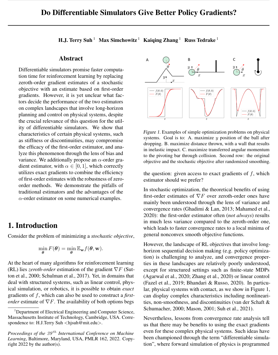
    In the paper's ball-and-wall optimization example, the pathwise estimate stalls in a flat region, whereas the score-function and alpha-order estimates reach minima; the interpolated estimate uses more pathwise information away from the discontinuity and favors the score estimate near it. In the angular-momentum-transfer example, following the pathwise estimate drives the solution out of a safe region after a discontinuity, while the score-function and alpha-order methods reach a robust local minimum. These examples support the paper's claim that estimator bias and finite-sample empirical bias can change which minimum gradient descent reaches, not merely the rate at which it approaches a shared minimum.

  9. Knowl 9 — Trajectory-optimization results depend on contact conditions

    empirical result

    The paper compares the three estimators in simulated trajectory-optimization tasks. In a pushing task with horizon H=200H=200, penalty-method contact, and viscous damping, the optimized input is a force sequence for moving a second block toward a goal. With a soft spring (k=10k=10), the pathwise estimate performs better than the score-function estimate; with a stiff spring (k=1000k=1000), the score-function estimate performs better. The alpha-order method adapts between them using the observed estimates and variances. In a friction task, the pathwise method initially converges faster but later degrades after the trajectory slides off a box; the score-function and alpha-order methods successfully optimize the trajectory, with the latter converging slightly faster. The results illustrate that stiffness and contact discontinuities affect which gradient estimate is useful.

  10. Knowl 10 — Tennis policy optimization exposes geometric discontinuities

    empirical result

    In a tennis-like task, a paddle policy must bounce a ball toward a target. The experiment uses a linear feedback policy with d=21d=21 parameters, horizon H=200H=200, and continuous event detection with a time-of-impact formulation to obtain pathwise derivatives. The score-function and alpha-order estimates find policies that direct balls from multiple initial conditions toward the target. The pathwise-only optimizer is affected by geometric discontinuities and continues to miss many balls; the alpha-order method converges slightly faster than the score-function method while retaining successful trajectories.

  11. Knowl 11 — The practical confidence bound is heuristic and pathwise gradients cost more

    limitation

    The alpha-order accuracy guarantee is conditional on having a valid confidence bound ε\varepsilon for the score-function estimate. The paper's practical Bernstein-based procedure substitutes an empirical variance estimate for the unknown variance and uses a chosen bound on sample deviations, even though Gaussian noise makes individual gradient samples unbounded. The authors therefore describe this implementation as not entirely rigorous; a statistically rigorous bound would need to handle both estimated variance and unbounded samples, and they conjecture that such a bound could be overly conservative. In addition, for the same number of trajectories, computing pathwise gradients costs more than computing score-function estimates because it requires automatic differentiation through the simulation.

Coverage note — Formal measure-theoretic proofs and supplementary technical lemmas were omitted because they support the stated estimator guarantees without adding independent contributions.

References

  1. 1.Agarwal, A., Kakade, S. M., Lee, J. D., and Mahajan, G. On the theory of policy gradient methods: Optimality, approximation, and distribution shift, 2020.
  2. 2.Bangaru, S. P., Michel, J., Mu, K., Bernstein, G., Li, T.-M., and Ragan-Kelley, J. Systematically differentiating parametric discontinuities. ACM Trans. Graph., 40(4), July 2021. ISSN 0730-0301. doi: 10.1145/3450626.3459775.
  3. 3.Berahas, A. S., Cao, L., Choromanski, K., and Scheinberg, K. A theoretical and empirical comparison of gradient approximations in derivative-free optimization. arXiv: Optimization and Control, 2019.
  4. 4.Bhandari, J. and Russo, D. Global optimality guarantees for policy gradient methods, 2020.
  5. 5.Boyd, S. and Vandenberghe, L. Convex optimization. Cambridge university press, 2004.
  6. 6.Carpentier, J., Saurel, G., Buondonno, G., Mirabel, J., Lamiraux, F., Stasse, O., and Mansard, N. The pinocchio c++ library : A fast and flexible implementation of rigid body dynamics algorithms and their analytical derivatives. In 2019 IEEE/SICE International Symposium on System Integration (SII), pp. 614–619, 2019. doi: 10.1109/SII.2019.8700380.
  7. 7.Castro, A. M., Qu, A., Kuppuswamy, N., Alspach, A., and Sherman, M. A transition-aware method for the simulation of compliant contact with regularized friction. IEEE Robotics and Automation Letters, 5(2):1859–1866, Apr 2020. ISSN 2377-3774. doi: 10.1109/lra.2020.2969933. URL http://dx.doi.org/10.1109/LRA.2020.2969933.
  8. 8.Çinlar, E. Probability and stochastics, volume 261. Springer, 2011.
  9. 9.Coumans, E. and Bai, Y. Pybullet, a python module for physics simulation for games, robotics and machine learning. http://pybullet.org, 2016–2021.
  10. 10.de Avila Belbute-Peres, F., Smith, K., Allen, K., Tenenbaum, J., and Kolter, J. Z. End-to-end differentiable physics for learning and control. In Bengio, S., Wallach, H., Larochelle, H., Grauman, K., Cesa-Bianchi, N., and Garnett, R. (eds.), Advances in Neural Information Processing Systems, volume 31. Curran Associates, Inc., 2018. URL https://proceedings.neurips.cc/paper/2018/file/842424a1d0595b76ec4fa03c46e8d755-Paper.pdf.
  11. 11.Du, T., Li, Y., Xu, J., Spielberg, A., Wu, K., Rus, D., and Matusik, W. D3{pg}: Deep differentiable deterministic policy gradients, 2020. URL https://openreview.net/forum?id=rkxZCJrtwS.
  12. 12.Duchi, J., Bartlett, P., and Wainwright, M. Randomized smoothing for stochastic optimization. SIAM Journal on Optimization, 22, 03 2011. doi: 10.1137/110831659.
  13. 13.Duchi, J., Jordan, M., Wainwright, M., and Wibisono, A. Optimal rates for zero-order convex optimization: The power of two function evaluations. IEEE Transactions on Information Theory, 61, 12 2015. doi: 10.1109/TIT.2015.2409256.
  14. 14.Elandt, R., Drumwright, E., Sherman, M., and Ruina, A. A pressure field model for fast, robust approximation of net contact force and moment between nominally rigid objects. IROS, pp. 8238–8245, 2019.
  15. 15.Ern, A. and Guermond, J.-L. Theory and practice of finite elements, volume 159. Springer Science & Business Media, 2013.
  16. 16.Fazel, M., Ge, R., Kakade, S. M., and Mesbahi, M. Global convergence of policy gradient methods for the linear quadratic regulator, 2019.
  17. 17.Freeman, C. D., Frey, E., Raichuk, A., Girgin, S., Mordatch, I., and Bachem, O. Brax - a differentiable physics engine for large scale rigid body simulation. In Thirty-fifth Conference on Neural Information Processing Systems Datasets and Benchmarks Track (Round 1), 2021. URL https://openreview.net/forum?id=VdvDlnnjzIN.
  18. 18.Geilinger, M., Hahn, D., Zehnder, J., Bächer, M., Thomaszewski, B., and Coros, S. Add: Analytically differentiable dynamics for multi-body systems with frictional contact, 2020.
  19. 19.Ghadimi, S. and Lan, G. Stochastic first- and zeroth-order methods for nonconvex stochastic programming. SIAM Journal on Optimization, 23(4):2341–2368, 2013. doi: 10.1137/120880811. URL https://doi.org/10.1137/120880811.
  20. 20.Gradu, P., Hallman, J., Suo, D., Yu, A., Agarwal, N., Ghai, U., Singh, K., Zhang, C., Majumdar, A., and Hazan, E. Deluca – a differentiable control library: Environments, methods, and benchmarking, 2021.
  21. 21.Howell, T. A., Cleac’h, S. L., Kolter, J. Z., Schwager, M., and Manchester, Z. Dojo: A differentiable simulator for robotics, 2022. URL https://arxiv.org/abs/2203.00806.
  22. 22.Hu, Y., Anderson, L., Li, T.-M., Sun, Q., Carr, N., Ragan-Kelley, J., and Durand, F. Difftaichi: Differentiable programming for physical simulation. ICLR, 2020.
  23. 23.Huang, Z., Hu, Y., Du, T., Zhou, S., Su, H., Tenenbaum, J. B., and Gan, C. Plasticinelab: A soft-body manipulation benchmark with differentiable physics. In International Conference on Learning Representations, 2021. URL https://openreview.net/forum?id=xCcdBRQEDW.
  24. 24.Hunt, K. H. and Crossley, F. R. E. Coefficient of Restitution Interpreted as Damping in Vibroimpact. Journal of Applied Mechanics, 42(2):440–445, 06 1975. ISSN 0021-8936. doi: 10.1115/1.3423596. URL https://doi.org/10.1115/1.3423596.
  25. 25.Kakade, S. M. On the sample complexity of reinforcement learning. University of London, University College London (United Kingdom), 2003.
  26. 26.Kingma, D. P., Salimans, T., and Welling, M. Variational dropout and the local reparameterization trick. In Cortes, C., Lawrence, N., Lee, D., Sugiyama, M., and Garnett, R. (eds.), Advances in Neural Information Processing Systems, volume 28. Curran Associates, Inc., 2015.
  27. 27.Lasota, A. and Mackey, M. C. Chaos, Fractals, and Noise: Stochastic Aspects of Dynamics. Cambridge university press, 1996.
  28. 28.Le Lidec, Q., Montaut, L., Schmid, C., Laptev, I., and Carpentier, J. Leveraging Randomized Smoothing for Optimal Control of Nonsmooth Dynamical Systems. working paper or preprint, December 2021. URL https://hal.archives-ouvertes.fr/hal-03480419.
  29. 29.Macklin, M., Müller, M., Chentanez, N., and Kim, T.-Y. Unified particle physics for real-time applications. ACM Trans. Graph., 33(4), jul 2014. ISSN 0730-0301. doi: 10.1145/2601097.2601152. URL https://doi-org.libproxy.mit.edu/10.1145/2601097.2601152.
  30. 30.Mahamed, S., Rosca, M., Figurnov, M., and Mnih, A. Monte carlo gradient estimation in machine learning. In Dy, J. and Krause, A. (eds.), Journal of Machine Learning Research, volume 21, pp. 1–63, 4 2020.
  31. 31.Mason, M. T. Mechanics of Robotic Manipulation. The MIT Press, 06 2001. ISBN 9780262256629. doi: 10.7551/mitpress/4527.001.0001. URL https://doi.org/10.7551/mitpress/4527.001.0001.
  32. 32.Maurer, A. and Pontil, M. Empirical bernstein bounds and sample variance penalization. arXiv preprint arXiv:0907.3740, 2009.
  33. 33.Metz, L., Maheswaranathan, N., Nixon, J., Freeman, D., and Sohl-Dickstein, J. Understanding and correcting pathologies in the training of learned optimizers. In Chaudhuri, K. and Salakhutdinov, R. (eds.), Proceedings of the 36th International Conference on Machine Learning, volume 97 of Proceedings of Machine Learning Research, pp. 4556–4565. PMLR, 09–15 Jun 2019.
  34. 34.Metz, L., Freeman, C. D., Schoenholz, S. S., and Kachman, T. Gradients are not all you need, 2021.
  35. 35.Mirtich, B. V. Impulse-Based Dynamic Simulation of Rigid Body Systems. PhD thesis, 1996. AAI9723116.
  36. 36.Mora, M. A. Z., Peychev, M., Ha, S., Vechev, M., and Coros, S. Pods: Policy optimization via differentiable simulation. In Meila, M. and Zhang, T. (eds.), Proceedings of the 38th International Conference on Machine Learning, volume 139 of Proceedings of Machine Learning Research, pp. 7805–7817. PMLR, 18–24 Jul 2021. URL https://proceedings.mlr.press/v139/mora21a.html.
  37. 37.Pang, T. A convex quasistatic time-stepping scheme for rigid multibody systems with contact and friction. 2021 IEEE International Conference on Robotics and Automation (ICRA), pp. 6614–6620, 2021.
  38. 38.Parmas, P., Rasmussen, C. E., Peters, J., and Doya, K. PIPPS: Flexible model-based policy search robust to the curse of chaos. In Dy, J. and Krause, A. (eds.), Proceedings of the 35th International Conference on Machine Learning, volume 80 of Proceedings of Machine Learning Research, pp. 4065–4074. PMLR, 10–15 Jul 2018.
  39. 39.Paszke, A., Gross, S., Massa, F., Lerer, A., Bradbury, J., Chanan, G., Killeen, T., Lin, Z., Gimelshein, N., Antiga, L., Desmaison, A., Kopf, A., Yang, E., DeVito, Z., Raison, M., Tejani, A., Chilamkurthy, S., Steiner, B., Fang, L., Bai, J., and Chintala, S. Pytorch: An imperative style, high-performance deep learning library. In Wallach, H., Larochelle, H., Beygelzimer, A., d’Alche Buc, F., Fox, E., and Garnett, R. (eds.), Advances in Neural Information Processing Systems 32, pp. 8024–8035. Curran Associates, Inc., 2019.
  40. 40.Rudin, W. et al. Principles of mathematical analysis, volume 3. Mcgraw-hill New York, 1964.
  41. 41.Schulman, J., Heess, N., Weber, T., and Abbeel, P. Gradient estimation using stochastic computation graphs. In Cortes, C., Lawrence, N., Lee, D., Sugiyama, M., and Garnett, R. (eds.), Advances in Neural Information Processing Systems, volume 28. Curran Associates, Inc., 2015.
  42. 42.Schulman, J., Wolski, F., Dhariwal, P., Radford, A., and Klimov, O. Proximal policy optimization algorithms, 2017.
  43. 43.Stein, E. M. and Shakarchi, R. Real analysis. Princeton University Press, 2009.
  44. 44.Stewart, D. and Trinkle, J. J. An implicit time-stepping scheme for rigid body dynamics with coulomb friction. volume 1, pp. 162–169, 01 2000. doi: 10.1109/ROBOT.2000.844054.
  45. 45.Stribeck, R. Die wesentlichen Eigenschaften der Gleit- und Rollenlager. Mitteilungen uber Forschungsarbeiten auf dem Gebiete des Ingenieurwesens, insbesondere aus den Laboratorien der technischen Hochschulen. Julius Springer, 1903.
  46. 46.Suh, H. J. T., Pang, T., and Tedrake, R. Bundled gradients through contact via randomized smoothing. arXiv preprint, 2021.
  47. 47.Sutton, R., Mcallester, D., Singh, S., and Mansour, Y. Policy gradient methods for reinforcement learning with function approximation. Adv. Neural Inf. Process. Syst, 12, 02 2000.
  48. 48.Tedrake, R. Drake: A planning, control, and analysis toolbox for nonlinear dynamical systems, 2022. URL http://drake.mit.edu.
  49. 49.Todorov, E., Erez, T., and Tassa, Y. Mujoco: A physics engine for model-based control. In IROS, pp. 5026–5033, 2012. doi: 10.1109/IROS.2012.6386109.
  50. 50.Tropp, J. A. An introduction to matrix concentration inequalities. Foundations and Trends® in Machine Learning, 8(1-2):1–230, 2015. ISSN 1935-8237. doi: 10.1561/2200000048. URL http://dx.doi.org/10.1561/2200000048.
  51. 51.van der Schaft, A. and Schumacher, H. An Introduction to Hybrid Dynamical Systems. Springer Publishing Company, Incorporated, 1st edition, 2000. ISBN 978-1-4471-3916-4.
  52. 52.Wasserman, L. All of statistics: a concise course in statistical inference, volume 26. Springer, 2004.
  53. 53.Werling, K., Omens, D., Lee, J., Exarchos, I., and Liu, C. K. Fast and feature-complete differentiable physics for articulated rigid bodies with contact, 2021.
  54. 54.Williams, R. J. Simple statistical gradient-following algorithms for connectionist reinforcement learning. Machine Learning, 3, 05 1992.
  55. 55.Zhang, K., Koppel, A., Zhu, H., and Başar, T. Global convergence of policy gradient methods to (almost) locally optimal policies, 2020.

Citation

MLA
Suh, H. J., et al. “Do Differentiable Simulators Give Better Policy Gradients?”. International Conference on Machine Learning, vol. 162, 2022, pp. 20668–96, https://proceedings.mlr.press/v162/suh22b.html.
APA
Suh, H. J., Simchowitz, M., Zhang, K., & Tedrake, R. (2022). Do Differentiable Simulators Give Better Policy Gradients?. International Conference on Machine Learning, 162, 20668–20696. https://proceedings.mlr.press/v162/suh22b.html
Chicago
Suh, H. J., M. Simchowitz, K. Zhang, and R. Tedrake. 2022. “Do Differentiable Simulators Give Better Policy Gradients?”. International Conference on Machine Learning 162: 20668–96. https://proceedings.mlr.press/v162/suh22b.html.
Harvard
Suh, H.J. et al. (2022) “Do Differentiable Simulators Give Better Policy Gradients?”, International Conference on Machine Learning. PMLR, pp. 20668–20696. Available at: https://proceedings.mlr.press/v162/suh22b.html.
Vancouver
1. Suh HJ, Simchowitz M, Zhang K, Tedrake R (2022) Do Differentiable Simulators Give Better Policy Gradients?. In: International Conference on Machine Learning. PMLR, pp 20668–20696

BibTeX

@InProceedings{pmlr-v162-suh22b,
  title = 	 {Do Differentiable Simulators Give Better Policy Gradients?},
  author =       {Suh, Hyung Ju and Simchowitz, Max and Zhang, Kaiqing and Tedrake, Russ},
  booktitle = 	 {Proceedings of the 39th International Conference on Machine Learning},
  pages = 	 {20668--20696},
  year = 	 {2022},
  editor = 	 {Chaudhuri, Kamalika and Jegelka, Stefanie and Song, Le and Szepesvari, Csaba and Niu, Gang and Sabato, Sivan},
  volume = 	 {162},
  series = 	 {Proceedings of Machine Learning Research},
  month = 	 {17--23 Jul},
  publisher =    {PMLR},
  pdf = 	 {https://proceedings.mlr.press/v162/suh22b/suh22b.pdf},
  url = 	 {https://proceedings.mlr.press/v162/suh22b.html},
  abstract = 	 {Differentiable simulators promise faster computation time for reinforcement learning by replacing zeroth-order gradient estimates of a stochastic objective with an estimate based on first-order gradients. However, it is yet unclear what factors decide the performance of the two estimators on complex landscapes that involve long-horizon planning and control on physical systems, despite the crucial relevance of this question for the utility of differentiable simulators. We show that characteristics of certain physical systems, such as stiffness or discontinuities, may compromise the efficacy of the first-order estimator, and analyze this phenomenon through the lens of bias and variance. We additionally propose an $\alpha$-order gradient estimator, with $\alpha \in [0,1]$, which correctly utilizes exact gradients to combine the efficiency of first-order estimates with the robustness of zero-order methods. We demonstrate the pitfalls of traditional estimators and the advantages of the $\alpha$-order estimator on some numerical examples.}
}
Metadata:DOI registry

Access the Paper

This paper is available from its original source. Click below to access the PDF.

Open PDF
License: https://creativecommons.org/licenses/by/4.0/