Tensor Completion for Estimating Missing Values in Visual Data

Ji LiuPrzemyslaw MusialskiPeter WonkaJieping Ye

article2009TPAMI2,104 citations

Establishes a foundational framework for low-rank tensor completion by defining the tensor trace norm and developing three efficient convex optimization algorithms (SiLRTC, FaLRTC, and HaLRTC) to accurately recover missing visual data from highly incomplete observations.

Listen

Modern computer vision and imaging applications frequently handle multi-dimensional visual datasets, such as color images, video sequences, medical scans, and reflectance data, that contain missing entries caused by sensor acquisition flaws, data compression, or the manual removal of unwanted objects. While traditional matrix methods can recover missing entries in two-dimensional data, they fail to simultaneously capture the rich, multi-way correlations across higher-dimensional structures. Existing tensor-based recovery techniques have largely relied on non-convex heuristic models that struggle to find global optimal solutions or require significant manual tuning.

The article establishes a convex optimization framework to accurately recover missing values in multi-dimensional visual datasets by introducing a mathematical definition for the trace norm of higher-order data arrays. The authors set out to formulate scalable, globally optimal algorithms for visual data completion and demonstrate their superior accuracy and efficiency across diverse real-world visual applications.

To evaluate this framework, the authors formulated the completion problem as a convex optimization model that minimizes a weighted combination of unfolded matrix trace norms. They designed three distinct algorithms: a simple coordinate descent approach, an accelerated smoothing gradient technique, and an exact augmented multiplier method. The authors validated these methods through synthetic data benchmarks across various dimensions and rank configurations, as well as real-world datasets including 3D brain magnetic resonance imaging (MRI), 2D building facade in-painting, color video sequence reconstruction, and 4D material reflectance data. Performance was measured by relative reconstruction error and computation runtime against traditional matrix completion, slice-wise recovery, and non-convex heuristic approaches.

The analysis yielded several key findings. First, the proposed convex tensor completion framework consistently outperformed non-convex heuristic models, particularly on higher-rank data and heavily degraded datasets where up to 80% to 90% of entries were missing. Second, tensor-based completion achieved substantially lower reconstruction errors than 2D matrix completion and slice-wise methods by simultaneously capturing correlations across all data dimensions. Third, among the proposed optimization techniques, the fast smoothing algorithm proved fastest for obtaining moderate-accuracy solutions (down to relative errors around 1%), whereas the high-accuracy multiplier method proved dramatically faster and superior when extremely precise solutions (relative errors down to one-millionth) were required. Finally, both advanced algorithms scaled efficiently, outperforming existing alternating direction methods from previous literature.

These findings demonstrate that multi-dimensional visual data can be accurately restored even with very limited sample observations. For organizational stakeholders, adopting trace-norm tensor completion reduces the risk of visual artifacts and data loss, lowers operational storage and bandwidth costs via aggressive data compression, and enhances workflow efficiency across automated quality control, medical diagnostics, and digital asset editing.

Organizations handling multi-dimensional imaging workflows should replace ad hoc 2D matrix recovery or heuristic tensor models with trace-norm optimization methods. Practitioners requiring fast rendering or rapid previewing should deploy the fast smoothing method, while workflows demanding high precision, such as medical scanning or archival restoration, should implement the high-accuracy multiplier method. In production environments, combining both approaches—initializing with the fast smoothing method and refining with the high-accuracy multiplier method—is recommended to optimize computational throughput.

Confidence in the reported experimental performance is high across low-rank synthetic and empirical visual domains. However, users should note that the methodology inherently relies on the underlying dataset exhibiting low-rank structural properties; performance may degrade on data lacking low-rank characteristics. Future initiatives should pursue formal theoretical recovery bounds for higher-order arrays and extend the framework to accommodate heavily corrupted data containing sparse outliers.

Arizona State University acquisition process coordinate descent heuristic approaches tensor completion low rank tensor completion algorithm matrix completion

Liu et al (2009).pdf

Book: Convex Optimization: Algorithms and Complexity, Sébastien Bubeck (2015). Mastering the foundational convex optimization principles and oracle complexities surveyed here is essential for understanding the convex tensor-completion formulations and trace norm minimization algorithms developed in the source.

Paper: TensoRF: Tensorial Radiance Fields, Anpei Chen et al. (2022). This paper extends the tensor-based modeling philosophy of the source by introducing TensoRF to decompose radiance fields into efficient tensorial representations for 3D scene reconstruction.

Cover for Tensor Completion for Estimating Missing Values in Visual Data

Abstract

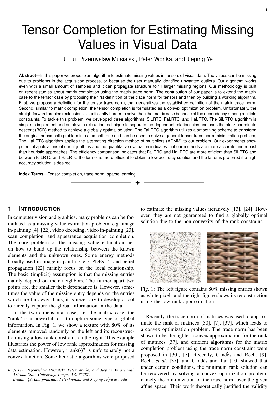
Abstract—In this paper we propose an algorithm to estimate missing values in tensors of visual data. The values can be missing due to problems in the acquisition process, or because the user manually identified unwanted outliers. Our algorithm works even with a small amount of samples and it can propagate structure to fill larger missing regions. Our methodology is built on recent studies about matrix completion using the matrix trace norm. The contribution of our paper is to extend the matrix case to the tensor case by proposing the first definition of the trace norm for tensors and then by building a working algorithm. First, we propose a definition for the tensor trace norm, that generalizes the established definition of the matrix trace norm. Second, similar to matrix completion, the tensor completion is formulated as a convex optimization problem. Unfortunately, the straightforward problem extension is significantly harder to solve than the matrix case because of the dependency among multiple constraints. To tackle this problem, we developed three algorithms: SiLRTC, FaLRTC, and HaLRTC. The SiLRTC algorithm is simple to implement and employs a relaxation technique to separate the dependant relationships and uses the block coordinate descent (BCD) method to achieve a globally optimal solution; The FaLRTC algorithm utilizes a smoothing scheme to transform the original nonsmooth problem into a smooth one and can be used to solve a general tensor trace norm minimization problem; The HaLRTC algorithm applies the alternating direction method of multipliers (ADMM) to our problem. Our experiments show potential applications of our algorithms and the quantitative evaluation indicates that our methods are more accurate and robust than heuristic approaches. The efficiency comparison indicates that FaLTRC and HaLRTC are more efficient than SiLRTC and between FaLRTC and HaLRTC the former is more efficient to obtain a low accuracy solution and the latter is preferred if a high accuracy solution is desired.

Topics

acquisition process coordinate descent heuristic approaches multiplier tensor factorization optimal solutions constrained optimization problems hybrid algorithms

Keywords

tensor completion low rank tensor completion algorithm matrix completion tensor trace norm minimization tensor factorization matrix rank minimization low rank approximation singular value decomposition Tucker model MRI brain data

1 INTRODUCTION
1.1 Notation
1.2 Organization
2 RELATED WORK
3 THE FORMULATION OF TENSOR COMPLETION
3.1 Convex Formulation for Tensor Completion
3.2 Three Heuristic Algorithm
4 A SIMPLE LOW RANK TENSOR COMPLETION (SILRTC) ALGORITHM
4.1 Simplified Formulation
4.2 The Main Algorithm
5 A FAST LOW RANK TENSOR COMPLETION (FALRTC) ALGORITHM
5.1 Smoothing Scheme
5.2 An Efficient Algorithm to Solve the Smooth Version
5.3 The FaLRTC Algorithm
6 A HIGH ACCURACY LOW RANK TENSOR COMPLETION (HALRTC) ALGORITHM
7 RESULTS
7.1 Model Comparison: Tensor Trace Norm Versus Heuristic Models
7.2 Model Comparison: Tensor Trace Norm Versus Matrix Trace Norm
7.3 Efficiency Comparison
7.4 Applications
8 CONCLUSION
ACKNOWLEDGMENTS
REFERENCES

Knowls

Knowl 1 — Tensor Trace Norm Definition
definition
Let $\mathcal{X} \in \mathbb{R}^{I_1 \times I_2 \times \dots \times I_n}$ be an $n$ -mode tensor. The mode- $i$ unfolding (matricization) of $\mathcal{X}$ , denoted by $\text{unfold}_i(\mathcal{X}) = X_{(i)} \in \mathbb{R}^{I_i \times (\prod_{k \neq i} I_k)}$ , is the matrix obtained by arranging the mode- $i$ fibers as columns.

The tensor trace norm (or nuclear norm) $\|\mathcal{X}\|_*$ is defined as the convex combination of the matrix trace norms of all unfolded matrices across each mode:

$\|\mathcal{X}\|_* := \sum_{i=1}^n \alpha_i \|X_{(i)}\|_*$

where $\alpha_i \ge 0$ are weights satisfying $\sum_{i=1}^n \alpha_i = 1$ , and $\|X_{(i)}\|_* = \sum_j \sigma_j(X_{(i)})$ denotes the standard matrix trace norm (the sum of singular values) of $X_{(i)}$ . When $n = 2$ , this definition reduces exactly to the matrix trace norm, because $\|X\|_* = \|X^T\|_*$ for any matrix $X$ .
Knowl 2 — Convex Formulation of Low-Rank Tensor Completion
model/method
Given an $n$ -mode observation tensor $\mathcal{T} \in \mathbb{R}^{I_1 \times I_2 \times \dots \times I_n}$ and an observed index subset $\Omega \subset \{1,\dots,I_1\} \times \dots \times \{1,\dots,I_n\}$ , the low-rank tensor completion problem seeks to recover missing entries by minimizing the tensor trace norm subject to consistency on observed entries:

$\min_{\mathcal{X}} \sum_{i=1}^n \alpha_i \|X_{(i)}\|_* \quad \text{s.t.} \quad \mathcal{X}_\Omega = \mathcal{T}_\Omega$

where $\mathcal{X} \in \mathbb{R}^{I_1 \times \dots \times I_n}$ is the recovered tensor, $X_{(i)}$ is its mode- $i$ unfolding, $\alpha_i \ge 0$ with $\sum_{i=1}^n \alpha_i = 1$ , and $\mathcal{X}_\Omega$ denotes the tensor whose elements in $\Omega$ equal those of $\mathcal{X}$ and are zero outside $\Omega$ .

Unlike the matrix case where the nuclear norm is the convex envelope of matrix rank, computing tensor rank for $n > 2$ is NP-hard. Thus, the weighted combination of matrix trace norms serves as a computationally tractable convex surrogate.
Knowl 3 — Simple Low Rank Tensor Completion Algorithm
algorithm
The Simple Low Rank Tensor Completion (SiLRTC) algorithm solves the tensor completion problem by relaxing the dependent matricization constraints. Auxiliary matrices $M_i \in \mathbb{R}^{I_i \times (\prod_{k \neq i} I_k)}$ are introduced with quadratic penalties:

$\min_{\mathcal{X}, M_1, \dots, M_n} \sum_{i=1}^n \left( \alpha_i \|M_i\|_* + \frac{\beta_i}{2} \|X_{(i)} - M_i\|_F^2 \right) \quad \text{s.t.} \quad \mathcal{X}_\Omega = \mathcal{T}_\Omega$

where $\alpha_i, \beta_i > 0$ . The algorithm alternates between solving for each $M_i$ via singular value thresholding and updating $\mathcal{X}$ via coordinate descent.

The singular value shrinkage operator is defined for a matrix $X = U \Sigma V^T$ as $\mathcal{D}_\tau(X) = U \text{diag}(\max(\sigma_j - \tau, 0)) V^T$ .
Input: Observed tensor $\mathcal{T}$ , index set $\Omega$ , initial $\mathcal{X}$ with $\mathcal{X}_\Omega = \mathcal{T}_\Omega$ , weights $\alpha_i$ , parameters $\beta_i$ , iterations $K$
Output: Recovered tensor $\mathcal{X}$
for $k = 1$ to $K$ do
    for $i = 1$ to $n$ do
         $M_i = \mathcal{D}_{\alpha_i / \beta_i}(X_{(i)})$
    end for
    for each index $(i_1, \dots, i_n)$ do
        if $(i_1, \dots, i_n) \notin \Omega$ then
             $\mathcal{X}_{i_1, \dots, i_n} = \frac{\sum_{i=1}^n \beta_i (\text{fold}_i(M_i))_{i_1, \dots, i_n}}{\sum_{i=1}^n \beta_i}$
        else
             $\mathcal{X}_{i_1, \dots, i_n} = \mathcal{T}_{i_1, \dots, i_n}$
        end if
    end for
end for
Knowl 4 — Nesterov Smoothing Scheme for Tensor Trace Norm Optimization
model/method
For a general objective $f(\mathcal{X}) = f_0(\mathcal{X}) + \sum_{i=1}^n \alpha_i \|X_{(i)}\|_*$ over a convex set $\mathcal{Q}$ , where $f_0(\mathcal{X})$ is smooth and convex, the nonsmooth trace norm terms are smoothed using Nesterov's smoothing technique. Using the dual characterization of the matrix trace norm $\|X\|_* = \max_{\|Y\| \le 1} \langle X, Y \rangle$ , a strongly convex quadratic regularizer $\frac{\mu_i}{2}\|Y_i\|_F^2$ with parameter $\mu_i > 0$ is subtracted in the dual space:

$f_\mu(\mathcal{X}) := f_0(\mathcal{X}) + \sum_{i=1}^n \max_{\|Y_i\| \le 1} \left( \alpha_i \langle \mathcal{X}, \mathcal{Y}_i \rangle - \frac{\mu_i}{2} \|\mathcal{Y}_i\|_F^2 \right)$

where $\|Y_i\|$ is the spectral norm of $Y_i = Y_{i(i)}$ . The gradient of $f_\mu(\mathcal{X})$ is given in closed form by:

$\nabla f_\mu(\mathcal{X}) = \nabla f_0(\mathcal{X}) + \sum_{i=1}^n \frac{\alpha_i^2}{\mu_i} \text{fold}_i \left( \mathcal{T}_{\frac{\mu_i}{\alpha_i}}(X_{(i)}) \right)$

where $\mathcal{T}_\tau(X) = U \text{diag}(\min(\sigma_j, \tau)) V^T$ denotes the singular value truncation operator for $X = U \Sigma V^T$ .
Knowl 5 — Fast Low Rank Tensor Completion Algorithm
algorithm
The Fast Low Rank Tensor Completion (FaLRTC) algorithm optimizes the smoothed tensor completion objective $f_\mu(\mathcal{X}) = \sum_{i=1}^n \max_{\|Y_{i(i)}\| \le 1} \left( \alpha_i \langle \mathcal{X}, \mathcal{Y}_i \rangle - \frac{\mu_i}{2}\|\mathcal{Y}_i\|_F^2 \right)$ over $\mathcal{Q} = \{\mathcal{X} \mid \mathcal{X}_\Omega = \mathcal{T}_\Omega\}$ using an accelerated gradient descent method with backtracking line search.

The gradient on $\mathcal{Q}$ evaluates to $(\nabla f_\mu(\mathcal{W}))_{i_1,\dots,i_n} = \sum_{i=1}^n \frac{\alpha_i^2}{\mu_i} (\text{fold}_i(\mathcal{T}_{\mu_i/\alpha_i}(W_{(i)})))_{i_1,\dots,i_n}$ for $(i_1,\dots,i_n) \notin \Omega$ , and $0$ for $(i_1,\dots,i_n) \in \Omega$ .
Input: Observation $\mathcal{T}$ , index set $\Omega$ , $\mathcal{X}$ with $\mathcal{X}_\Omega = \mathcal{T}_\Omega$ , $c \in (0, 1)$ , iterations $K$ , smoothing parameters $\mu_i$ , initial Lipschitz estimate $L$
Output: Recovered tensor $\mathcal{X}$
Initialize $\mathcal{Z} = \mathcal{W} = \mathcal{X}$ , $L' = L$ , $B = 0$
for $k = 0$ to $K$ do
    while true do
         $\theta = \frac{L}{2L'}(1 + \sqrt{1 + 4L' B})$
         $\mathcal{W} = \frac{\theta / L}{B + \theta / L}\mathcal{Z} + \frac{B}{B + \theta / L}\mathcal{X}$
        if $f_\mu(\mathcal{X}) \le f_\mu(\mathcal{W}) - \frac{\|\nabla f_\mu(\mathcal{W})\|_F^2}{2L'}$ then
            break
        end if
         $\mathcal{X}' = \mathcal{W} - \frac{1}{L'}\nabla f_\mu(\mathcal{W})$
        if $f_\mu(\mathcal{X}') \le f_\mu(\mathcal{W}) - \frac{\|\nabla f_\mu(\mathcal{W})\|_F^2}{2L'}$ then
             $\mathcal{X} = \mathcal{X}'$
            break
        end if
         $L' = L' / c$
    end while
     $L = L'$
     $\mathcal{Z} = \mathcal{Z} - \frac{\theta}{L} \nabla f_\mu(\mathcal{W})$
     $B = B + \frac{\theta}{L}$
end for
Knowl 6 — Convergence Rate for the FaLRTC Algorithm
theoretical result
Let $\mathcal{X}^*$ denote an optimal solution to the nonsmooth problem $\min_{\mathcal{X} \in \mathcal{Q}} f(\mathcal{X}) = f_0(\mathcal{X}) + \sum_{i=1}^n \alpha_i \|X_{(i)}\|_*$ , where $f_0(\mathcal{X})$ is smooth and convex with Lipschitz constant $\bar{L}$ , and $\mathcal{Q}$ is a convex set (which can be unbounded). Let $\mathcal{X}^0$ be the initial point and let $D$ be a positive constant such that:

$D \ge \min_{\mathcal{X}^*} \|\mathcal{X}^* - \mathcal{X}^0\|_F$

If the smoothing parameters are chosen according to:

$\mu_i = \frac{2 \alpha_i D}{K \sqrt{c I_i}}$

for line-search constant $c \in (0, 1)$ , mode dimension $I_i$ , and total iteration count $K$ , then the output $\mathcal{X}^K$ of the FaLRTC algorithm satisfies:

$f(\mathcal{X}^K) - f(\mathcal{X}^*) \le \frac{2\bar{L}}{c}\left( \frac{D}{K} \right)^2 + \frac{2D}{K} \sum_{i=1}^n \frac{\alpha_i \sqrt{I_i}}{\sqrt{c}}$

This guarantees an $O(K^{-1})$ convergence rate on the original nonsmooth objective function, and implies the parameter ratio $\mu_1 : \mu_2 : \dots : \mu_n = \frac{\alpha_1}{\sqrt{I_1}} : \frac{\alpha_2}{\sqrt{I_2}} : \dots : \frac{\alpha_n}{\sqrt{I_n}}$ .
Knowl 7 — High Accuracy Low Rank Tensor Completion Algorithm
algorithm
The High Accuracy Low Rank Tensor Completion (HaLRTC) algorithm solves the exact noiseless tensor completion problem using the Alternating Direction Method of Multipliers (ADMM) without relaxing equality constraints. It introduces auxiliary tensors $\mathcal{M}_1, \dots, \mathcal{M}_n$ and Lagrangian multipliers $\mathcal{Y}_1, \dots, \mathcal{Y}_n$ for the augmented Lagrangian:

$L_\rho(\mathcal{X}, \mathcal{M}_1, \dots, \mathcal{M}_n, \mathcal{Y}_1, \dots, \mathcal{Y}_n) = \sum_{i=1}^n \left( \alpha_i \|M_{i(i)}\|_* + \langle \mathcal{X} - \mathcal{M}_i, \mathcal{Y}_i \rangle + \frac{\rho}{2}\|\mathcal{M}_i - \mathcal{X}\|_F^2 \right)$

where $\mathcal{D}_\tau(X) = U \text{diag}(\max(\sigma_j - \tau, 0)) V^T$ is the singular value shrinkage operator.
Input: Observed tensor $\mathcal{T}$ , index set $\Omega$ , penalty parameter $\rho$ , step multiplier $t \in [1.1, 1.2]$ , iterations $K$
Output: Recovered tensor $\mathcal{X}$
Initialize $\mathcal{X}_\Omega = \mathcal{T}_\Omega$ , $\mathcal{X}_{\Omega^c} = 0$ , and $\mathcal{Y}_i = 0$ for all $i = 1, \dots, n$
for $k = 0$ to $K$ do
    for $i = 1$ to $n$ do
         $\mathcal{M}_i = \text{fold}_i\left( \mathcal{D}_{\alpha_i / \rho} \left( X_{(i)} + \frac{1}{\rho} Y_{i(i)} \right) \right)$
    end for
     $\mathcal{X}_{\Omega^c} = \left( \frac{1}{n} \sum_{i=1}^n \left( \mathcal{M}_i - \frac{1}{\rho}\mathcal{Y}_i \right) \right)_{\Omega^c}$
     $\mathcal{X}_\Omega = \mathcal{T}_\Omega$
    for $i = 1$ to $n$ do
         $\mathcal{Y}_i = \mathcal{Y}_i - \rho (\mathcal{M}_i - \mathcal{X})$
    end for
     $\rho = t \cdot \rho$
end for
Knowl 8 — Non-Convex Heuristic Baselines for Tensor Completion
model/method
Three heuristic, non-convex baseline formulations for tensor completion are defined for comparison with convex tensor trace norm minimization:
1. Tucker Model Completion: Factorizes the tensor into a core tensor $\mathcal{C} \in \mathbb{R}^{r_1 \times \dots \times r_n}$ and factor matrices $U_i \in \mathbb{R}^{I_i \times r_i}$ : $\min_{\mathcal{X}, \mathcal{C}, U_1, \dots, U_n} \frac{1}{2} \|\mathcal{X} - \mathcal{C} \times_1 U_1 \times_2 \dots \times_n U_n\|_F^2 \quad \text{s.t.} \quad \mathcal{X}_\Omega = \mathcal{T}_\Omega$
2. PARAFAC Model Completion: Factorizes the tensor into rank-1 outer product components using $U_i \in \mathbb{R}^{I_i \times r}$ : $\min_{\mathcal{X}, U_1, \dots, U_n} \frac{1}{2} \|\mathcal{X} - U_1 \circ U_2 \circ \dots \circ U_n\|_F^2 \quad \text{s.t.} \quad \mathcal{X}_\Omega = \mathcal{T}_\Omega$
3. Unfolded SVD Rank Constraint: Constrains the rank of each mode unfolding independently: $\min_{\mathcal{X}, M_1, \dots, M_n} \frac{1}{2} \sum_{i=1}^n \|X_{(i)} - M_i\|_F^2 \quad \text{s.t.} \quad \mathcal{X}_\Omega = \mathcal{T}_\Omega, \; \text{rank}(M_i) \le r_i, \; i = 1, \dots, n$
All three formulations are non-convex and are solved via block coordinate descent, which is sensitive to initialization and prone to local minima.

Knowl 9 — Empirical Recovery Performance: Tensor Trace Norm vs Heuristic and Matrix Completion

empirical result

On brain MRI data of size $181 \times 217 \times 181$ (with approximate unfolding ranks $[35, 42, 36]$ ) and synthetic low-rank tensors, convex tensor trace norm minimization via SiLRTC, FaLRTC, and HaLRTC consistently outperforms the non-convex heuristic models (Tucker, PARAFAC, SVD) and 2D matrix completion baselines (both matricized completion and slice-wise completion S-MC), especially under severe missing data.

Samples	Tucker	Parafac	SVD	SiLRTC $\gamma=10^4$	SiLRTC $\gamma=10^3$	SiLRTC $\gamma=10^2$	SiLRTC $\gamma=10$	FaLRTC	HaLRTC
20%	371	234	274	309	47	22	21	17	16
50%	65	58	62	101	12	2	0	0	0
80%	21	45	16	40	4	1	0	0	0

Relative Standard Error ( $\text{RSE} = \|\mathcal{X} - \mathcal{T}\|_F / \|\mathcal{T}\|_F \times 10^{-4}$ ) on brain MRI shows that at 20% sample rate, FaLRTC ( $17 \times 10^{-4}$ ) and HaLRTC ( $16 \times 10^{-4}$ ) achieve an order-of-magnitude lower error than Tucker ( $371 \times 10^{-4}$ ), PARAFAC ( $234 \times 10^{-4}$ ), and SVD ( $274 \times 10^{-4}$ ). In slice-wise matrix completion on $60 \times 60 \times 60$ tensors with 20% samples, matrix completion produces RSE $> 0.22$ , whereas FaLRTC achieves RSE $\le 0.0001$ .

Knowl 10 — Efficiency Trade-offs among SiLRTC, FaLRTC, and HaLRTC
empirical result
Experimental comparison of computational efficiency on synthetic tensors of size $100 \times 100 \times 100$ ( $r_1=r_2=r_3=2$ ) and $50 \times 50 \times 50 \times 50$ ( $r_1=r_2=r_3=r_4=2$ ) with 20% observed samples shows distinct efficiency regimes:
1. Moderate/Low Accuracy ( $\text{RSE} \ge 10^{-2}$ ): FaLRTC is the fastest algorithm. For a 4-mode tensor achieving $\text{RSE} = 10^{-1}$ ( $20\text{ dB}$ SNR), FaLRTC requires $\sim 25.4\text{ s}$ , outperforming HaLRTC ( $\sim 35.0\text{ s}$ ), ADM-TR ( $\sim 199.0\text{ s}$ ), and SiLRTC ( $\sim 398.8\text{ s}$ ).
2. High Precision ( $\text{RSE} \le 10^{-4}$ to $10^{-6}$ ): HaLRTC is substantially more efficient than all competitors. For achieving $\text{RSE} = 10^{-6}$ ( $120\text{ dB}$ SNR) on the 3-mode tensor, HaLRTC converges in $22.3\text{ s}$ , whereas FaLRTC, SiLRTC, and ADM-TR fail to reach this precision within 100 seconds.
3. Practical Strategy: Combining FaLRTC for rapid initial descent followed by HaLRTC for high-precision convergence provides the best overall computational performance.
Knowl 11 — Methodological Limitations of Convex Tensor Completion
limitation
The low-rank tensor completion methods carry three primary limitations:
1. Low-Rank Structural Assumption: The framework assumes that the underlying tensor has approximate or exact low rank when matricized along each mode. Visual data lacking global multilinear correlation may not be recovered accurately.
2. Absence of Theoretical Exact Recovery Bounds: Unlike matrix completion, where nuclear norm minimization has proved exact recovery guarantees with tight incoherence bounds, theoretical sampling complexity bounds for exact tensor recovery under the proposed tensor trace norm were not established.
3. Per-Iteration SVD Computational Overhead: Each iteration in SiLRTC, FaLRTC, and HaLRTC requires computing singular value decompositions of $n$ unfolded matrices of dimension $I_i \times \prod_{k \neq i} I_k$ , which scales poorly for high tensor orders $n$ or very large mode dimensions.

Coverage note — Specific visual application demonstrations (image facade in-painting, video frame completion, and 4D BRDF reflectance estimation) were omitted as standalone knowls because they represent direct qualitative use cases of the core algorithms rather than distinct methodological contributions.

References

1.Y. Amit, M. Fink, N. Srebro, and S. Ullman. Uncovering shared structures in multiclass classification. ICML, pages 17–24, 2007.
2.A. Argyriou, T. Evgeniou, and M. Pontil. Multi-task feature learning. NIPS, pages 243–272, 2007.
3.F. R. Bach. Consistency of trace norm minimization. Journal of Machine Learning Research, 9:1019–1048, 2008.
4.M. Bertalmio, G. Sapiro, V. Caselles, and C. Ballester. Image inpainting. SIGGRAPH, pages 414–424, 2000.
5.S. Boyd, N. Parikh, E. Chu, B. Peleato, and J. Eckstein. Distributed optimization and statistical learning via the alternating direction method and multipliers. Unpublished, 2011.
6.J. Cai. Fast singular value thresholding without singular value decomposition. UCLA CAM Report, 2010.
7.J.-F. Cai, E. J. Candes, and Z. Shen. A singular value thresholding ` algorithm for matrix completion. SIAM Journal on Optimization, 20(4):1956–1982, 2010.
8.E. J. Candes, X. Li, Y. Ma, and J. Wright. Robust principal ` component analysis? Joural of the ACM, 58(1):1–37, 2009.
9.E. J. Candes and B. Recht. Exact matrix completion via convex ` optimization. Foundations of Computational Mathematics, 9(6):717– 772, 2009.
10.E. J. Candes and T. Tao. The power of convex relaxation: Near- ` optimal matrix completion. IEEE Transactions on Information Theory, 56(5):2053–2080, 2009.
11.L. Elden. Matrix Methods in Data Mining and Pattern Recgonition. 2007.
12.M. Fazel. Matrix rank minimization with applications. PhD thesis, Stanford University.
13.M. Fazel, H. Hindi, and S. Boyd. A rank minimization heuristic with application to minimum order system approximation. ACC, pages 4734–4739, 2001.
14.S. Gandy, B. Recht, and I. Yamada. Tensor completion and low-n-rank tensor recovery via convex optimization. Inverse Problem, 27, 2011.
15.D. Gross, Y.-K. Liu, S. T. Flammia, S. Becker, and J. Eisert. Quantum state tomography via compressed sensing. http//arxiv.org/abs/0909.3304, 2009.
16.L. Guo, Y. Li, J. Yang, and L. Lu. Hole-filling by rank sparsity tensor decomposition for medical imaging. IEICE, pages 1–4, 2010.
17.R. A. Harshman. Foundations of the parafac procedure: models and conditions for an "explanatory" multi-modal factor analysis. UCLA Working Papers in Phonetics, 16:1–84, 1970.
18.C. J. Hillar and L. heng Lim. Most tensor problems are np hard. CoRR, abs/0911.1393, 2009.
19.S. Ji, L. Sun, R. Jin, and J. Ye. Multi-label multiple kernel learning. NIPS, pages 777–784, 2008.
20.S. Ji and J. Ye. An accelerated gradient method for trace norm minimization. ICML, pages 457–464, 2009.
21.R. Keshavan, A. Montanari, and S. Oh. Matrix completion from a few entries. IEEE Transaction on Information Theory, abs/0901.3150, 2010.
22.N. Komodakis and G. Tziritas. Image completion using global optimization. CVPR, pages 417–424, 2006.
23.T. Korah and C. Rasmussen. Spatiotemporal inpainting for recovering texture maps of occluded building facades. IEEE Transactions on Image Processing, 16:2262–2271, 2007.
24.M. Kurucz, A. A. Benczur, and K. Csalogany. Methods for large scale svd with missing values. KDD, pages 31–38, 2007.
25.N. Li and B. Li. Tensor completion for on-board compression of hyperspectral images. ICIP, pages 517–520, 2010.
26.Y. Li, J. Yan, Y. Zhou, and J. Yang. Optimum subspace learning and error correction for tensors. ECCV, 2010.
27.Y. Li, Y. Zhou, J. Yan, J. Yang, and X. He. Tensor error correction for corrupted values in visual data. ICIP, pages 2321–2324, 2010.
28.Z. Lin, M. Chen, and Y. Ma. The augmented lagrange multiplier method for exact recovery of corrupted low-rank matrices. Technical Report UILU-ENG-09-2215, UIUC, (arXiv: 1009.5055), 2009.
29.J. Liu, P. Musialski, P. Wonka, and J. Ye. Tensor completion for estimating missing values in visual data. ICCV, pages 2114–2121, 2009.
30.S. Ma, D. Goldfarb, and L. Chen. Fixed point and bregman iterative methods for matrix rank minimization. Mathematical Programming, 128(1):321–353, 2009.
31.A. Nemirovski. Efficient methods in convex programming. 1995.
32.Y. Nesterov. A method of solving a convex programing problem with convergence rate o(1/k2). Soviet Mathematics Doklady, 27(2), 1983.
33.Y. Nesterov. Introductory lectures on convex programming. Lecture Notes, pages 119–120, 1998.
34.Y. Nesterov. Smooth minimization of non-smooth functions. Mathemtaical Programming, 103(1):127–152, 2005.
35.T. K. Pong, P. Tseng, S. Ji, and J. Ye. Trace norm regularization: Reformulations, algorithms, and multi-task learning. SIAM Journal on Optimization, 20(6):3465–3489, 2010.
36.B. Recht. A simpler approach to matrix completion. Journal of Machine Learning Research, 11:2287–2322, 2010.
37.B. Recht, M. Fazel, and P. A. Parrilo. Guaranteed minimum-rank solutions of linear matrix equations via nuclear norm minimization. SIAM Review, 52(3):471–501, 2010.
38.M. Signoretto, L. D. Lathauwer, and J. A. K. Suykens. Nuclear norms for tensors and their use for convex multilinear estimation. Submitted to Linear Algebra and Its Applications, 2010.
39.N. Srebro, J. D. M. Rennie, and T. S. Jaakkola. Maximum-margin matrix factorization. NIPS, pages 1329–1336, 2005.
40.J. F. Sturm. Using sedumi 1.02, a matlab toolbox for optimization over symmetric cones. Optimization Methods and Software, 11:623– 625, 1998.
41.K. C. Toh, M. J. Todd, and R. H. Tutuncu. Sdpt3: a matlab software package for semidefinite programming. Optimization Methods and Software, 11:545–581, 1999.
42.M. Tomasi and T. Kanade. Shape and motion from image stream under orthography: a factorization method. International Journal of Computer Vision, 9:137–154, 1992.
43.R. Tomioka, K. Hayashi, and H. Kashima. Estimation of low-rank tensors via convex optimization. arxiv.org/abs/1010.0789, 2011.
44.O. Troyanskaya, M. Cantor, G. Sherlock, P. Brown, T. Hastie, R. Tibshirani, D. Botstein, and R. B. Altman. Missing value estimation methods for dna microarrays. Bioinformatics, 17:520– 525, 2001.
45.P. Tseng. Convergence of block coordinate descent method for nondifferentiable minimization. Journal of Optimization Theory Application, 109:475–494, 2001.
46.L. R. Tucker. Some mathematical notes on three-mode factor analysis. Psychometrika, 31:279–311, 1966.
47.J. Yan, J. Liu, Y. Li, Z. Niu, and Y. Liu. Visual saliency detection via rank-sparsity decomposition. ICIP, pages 1089–1092, 2010.
48.Z. Zhou, X. Li, J. Wright, E. J. Candes, and Y. Ma. Stable principal ` component pursuit. CoRR, abs/1001.2363, 2010.

Citation

MLA

Liu, J., et al. “Tensor Completion for Estimating Missing Values in Visual Data”. IEEE Transactions on Pattern Analysis and Machine Intelligence, vol. 35, no. 1, 2013, pp. 208–20, https://doi.org/10.1109/TPAMI.2012.39.

APA

Liu, J., Musialski, P., Wonka, P., & Ye, J. (2013). Tensor Completion for Estimating Missing Values in Visual Data. IEEE Transactions on Pattern Analysis and Machine Intelligence, 35(1), 208–220. https://doi.org/10.1109/TPAMI.2012.39

Chicago

Liu, J., P. Musialski, P. Wonka, and J. Ye. 2013. “Tensor Completion for Estimating Missing Values in Visual Data”. IEEE Transactions on Pattern Analysis and Machine Intelligence 35 (1): 208–20. https://doi.org/10.1109/TPAMI.2012.39.

Harvard

Liu, J. et al. (2013) “Tensor Completion for Estimating Missing Values in Visual Data”, IEEE Transactions on Pattern Analysis and Machine Intelligence, 35(1), pp. 208–220. Available at: https://doi.org/10.1109/TPAMI.2012.39.

Vancouver

1. Liu J, Musialski P, Wonka P, Ye J (2013) Tensor Completion for Estimating Missing Values in Visual Data. IEEE Transactions on Pattern Analysis and Machine Intelligence 35:208–220

BibTeX

@article{Liu_2013, title={Tensor Completion for Estimating Missing Values in Visual Data}, volume={35}, ISSN={2160-9292}, url={http://dx.doi.org/10.1109/TPAMI.2012.39}, DOI={10.1109/tpami.2012.39}, number={1}, journal={IEEE Transactions on Pattern Analysis and Machine Intelligence}, publisher={Institute of Electrical and Electronics Engineers (IEEE)}, author={Liu, Ji and Musialski, Przemyslaw and Wonka, Peter and Ye, Jieping}, year={2013}, month=Jan, pages={208–220} }

Metadata:Crossref

Access the Paper

This paper is available from its original source. Click below to access the PDF.

Open PDF

Tensor Completion for Estimating Missing Values in Visual Data

Abstract

Topics

Keywords

Table of Contents

Knowls

Knowl 1 — Tensor Trace Norm Definition

Knowl 2 — Convex Formulation of Low-Rank Tensor Completion

Knowl 3 — Simple Low Rank Tensor Completion Algorithm

Knowl 4 — Nesterov Smoothing Scheme for Tensor Trace Norm Optimization

Knowl 5 — Fast Low Rank Tensor Completion Algorithm

Knowl 6 — Convergence Rate for the FaLRTC Algorithm

Knowl 7 — High Accuracy Low Rank Tensor Completion Algorithm

Knowl 8 — Non-Convex Heuristic Baselines for Tensor Completion

Knowl 9 — Empirical Recovery Performance: Tensor Trace Norm vs Heuristic and Matrix Completion

Knowl 10 — Efficiency Trade-offs among SiLRTC, FaLRTC, and HaLRTC

Knowl 11 — Methodological Limitations of Convex Tensor Completion

References

Citation

BibTeX

Access the Paper