Finetuning with Sampling: SFT Learns Better Than You Think cover

📄 Executive Summary

Organizations training frontier language models face a persistent dilemma when attempting to teach models new capabilities without degrading their existing skills. Supervised finetuning can incorporate rich, external expert solutions but commonly triggers catastrophic forgetting and poor generalization. In contrast, reinforcement learning preserves prior skills well but relies heavily on a model's ability to find correct solutions on its own, making it ineffective for complex problems that the base model cannot already solve.

The article introduces and evaluates a pre-training data transformation framework called projection sampling. The objective is to determine whether transforming external expert demonstration data into trajectories that closely match the base model's internal distribution can allow standard supervised finetuning to achieve strong generalization while preventing the degradation of prior capabilities.

The authors designed a sampling algorithm based on Markov chain Monte Carlo methods, specifically a blockwise Metropolis-Hastings technique. The algorithm takes external expert demonstrations and iteratively rewrites them in the base model's own style while preserving factual and logical correctness. The researchers evaluated this method across scientific reasoning (chemistry), advanced mathematical problem-solving, and clinical medical question answering using open-weight models ranging from 3 billion to 7 billion parameters (Qwen2.5 and Olmo-3). They benchmarked the approach against standard supervised finetuning, reinforcement learning algorithms, and on-policy self-distillation techniques.

The investigation produced several key findings. First, supervised finetuning on sampled data substantially improved task generalization, raising chemistry accuracy on Qwen2.5-7B by 31.7 percentage points and outperforming self-distillation by 4.2 percentage points. Second, the method dramatically reduced catastrophic forgetting; on the chemistry task, average performance loss on prior benchmarks dropped to just 1.1%, and in medical reasoning, it prevented a 16.3% capability drop seen in standard supervised finetuning. Third, in advanced mathematics, the approach improved MATH500 performance by 33.7 percentage points over the base model, beating the next-best reinforcement learning baseline by 26.9 percentage points. Fourth, models finetuned on this transformed data served as superior starting checkpoints for subsequent reinforcement learning, achieving the highest overall benchmark scores. Finally, the analysis showed that models learned fundamentally new capabilities rather than merely sharpening pre-existing behaviors, successfully solving difficult problems that the base model failed completely.

These findings suggest that data distribution alignment, rather than the choice between supervised finetuning and reinforcement learning, is the primary driver of effective post-training. For engineering and product leaders, this demonstrates that expensive and complex reinforcement learning pipelines can often be replaced or streamlined by using sampling as a one-time preprocessing step on training data, lowering runtime complexity and stabilizing training.

Teams developing domain-specific models should consider adopting projection sampling as an upfront data preparation primitive before supervised finetuning. If high-end reasoning performance is required, practitioners should initialize reinforcement learning from these sampled-finetuned models. When deploying this workflow, teams must ensure that the sampling transformation is performed specifically with the target base model, as data transformed for one model architecture does not transfer effectively to another.

Decision-makers should note certain limitations: the sampling step incurs an upfront computational cost during data preparation, and semantic verification in unstructured domains relies on automated language model evaluators. Nonetheless, given consistent empirical validation across multiple model families and diverse reasoning domains, confidence in the core methodology remains high.

📚 What to read before this

SFT Memorizes, RL Generalizes: A Comparative Study of Foundation Model Post-training, Tianzhe Chu et al. (2025). Its controlled comparison of SFT and RL on out-of-distribution tasks establishes the generalization-versus-memorization premise that this chapter directly revisits.
Preference Fine-Tuning of LLMs Should Leverage Suboptimal, On-Policy Data, Fahim Tajwar et al. (2024). Its analysis of when on-policy sampling matters for preference fine-tuning clarifies the sampling and data-distribution challenge this chapter addresses for SFT.

📚 What to read after this

Latent On-Policy Self-Distillation, Guibin Zhang et al. (2026). It extends on-policy learning from student-generated rollouts by learning how to encode privileged past successes into teacher guidance.
Trajectory-Refined Distillation, Li Jiang et al. (2026). It continues the focus on shaping on-policy training trajectories, refining sampled rollouts before distillation to correct errors that ordinary token-level supervision misses.
Self-Distillation Enables Continual Learning, Idan Shenfeld et al. (2026). It carries the combination of demonstrations and on-policy learning into continual skill and knowledge acquisition, testing how that approach can limit forgetting.

Finetuning with Sampling: SFT Learns Better Than You Think

Aayush Karan

^{1}

, Sitan Chen

^{1}

, Yilun Du

^{1}

^{1}

Harvard University

🌐 Website GitHub Code

Abstract

Introducing new capabilities to frontier models has long been the goal of posttraining, which predominantly employs supervised finetuning (SFT) and reinforcement learning (RL) to this end. Conventional wisdom dictates that RL enables strong generalization on new tasks without losing existing capabilities, while SFT is prone to weak generalization and catastrophic forgetting. At the same time, SFT can learn from off-policy expert data, whereas RL must rely on a model's ability to find successful trajectories with repeated sampling. In our work, we seek to leverage the strength of on-policy learning while utilizing the privileged information contained in off-policy data. However, rather than modifying the learning objective to accommodate this data, we instead tailor the data distribution to better suit the learner. We introduce a Markov chain Monte Carlo (MCMC) sampling algorithm that progressively transforms off-policy traces to be more on-policy given a reference model for finetuning. Across tasks like scientific skill acquisition, mathematical reasoning, and open-ended expertise, our sampling algorithm enables SFT to rival prevailing posttraining techniques, often generalizing better and forgetting less than strong on-policy baselines. In addition, the resulting finetuned models exhibit strong distributional performance and are capable of learning beyond sharpening the base model distribution. At a higher level, our approach presents sampling as a model-native operator that shapes data for learnability, offering broader utility as a general-purpose primitive throughout the posttraining stack.

1. Introduction

Posttraining has brought about revolutionary advances in the capabilites of frontier large language models (LLMs) ([1, 2]), giving sizeable performance gains across domains like math, science, and coding ([3, 4, 5]).

Still, a key open question remains: how can we introduce fundamentally new capabilities during posttraining without giving up existing ones? A large body of recent literature has been dedicated to understanding the extent to which existing learning frameworks – i.e., supervised finetuning (SFT) and reinforcement learning (RL) – can achieve this end. Overwhelming evidence ([6, 7, 8]) points towards RL as the paradigm of choice, citing superior generalization on unseen domains that appears to leave prior abilities intact. Meanwhile, SFT suffers from weak generalization and catastrophic forgetting ([9, 10]): a phenomenon where finetuned models exhibit significant deterioration in existing capabilities.

[6, 8] attribute this performance gap to the on-policy nature of RL: the model's own samples dictate learning updates, constraining finetuning towards distributions that do not stray far from the original starting point. SFT on the other hand is off-policy, leaving finetuning more susceptible to drastic updates and shifts in behavior ([11]).

At the same time, learning strictly on-policy is also a limitation, as it relies on the model's own ability to find successful trajectories through repeated sampling. If the model cannot generate a correct rollout on a training sample, there is no collective variance in reward, resulting in no learning signal. [12] observes this deficiency in practice, identifying a sizeable regime of hard training samples that are effectively discarded during RL as they are simply too difficult to yield any trainability.

This limitation is not ideal for the purposes of introducing new capabilities, where the model is unlikely to already be competent enough to produce a successful trajectory. Here SFT has an advantage, as it leverages trajectories constructed from off-policy privileged information that provide rich supervision signal without necessitating an explicit reward.

In this work, rather than modifying the learning algorithm to accommodate off-policy data, we ask if we can instead shape the data distribution to accommodate learning. More precisely, can we algorithmically sample on-policy trajectories that remain faithful to privileged off-policy information? To this end, we propose a sampling algorithm that progressively transforms a dataset of off-policy expert traces to be distributionally closer to a given base model distribution.

Figure 1: Composed with sampling, SFT can generalize better and forget less than on-policy learning. Left: we compare SFT composed with our sampling algorithm for off-policy data against SFT on the original dataset and an on-policy learning algorithm that integrates off-policy data into self-distillation (OPSD) ([13]). We illustrate this on the task of scientific reasoning for chemistry problems and plot performance on prior capabilities introduced during pretraining (MMLU and AMC). Right: we compare the three along two axes: new task accuracy (chemistry) and prior task retention, which measures the percent of base model performance the finetuned models are able to maintain. SFT composed with sampling performs the best on both axes.

Remarkably, this sampling step enables SFT to rival prevailing posttraining techniques, often generalizing better and forgetting less than strong on-policy learning algorithms.

Our contributions can be summarized as follows:

We introduce a framework that formalizes the task of transforming off-policy data into on-policy data for finetuning. Namely, given a base model and a dataset of expert trajectories, we specify a target data generation policy that preserves the information content of the original dataset while maintaining maximal proximity to the base model distribution.
To generate boosted samples from this policy, we introduce projection sampling, an approximate sampling algorithm using Markov chain Monte Carlo (MCMC) techniques that iteratively refine expert trajectories according to their likelihoods with respect to the base model.
We empirically demonstrate the effectiveness of our sampling procedure for SFT over a range of tasks, including scientific skill acquisition, mathematical reasoning, and open-ended expertise. Our results show that SFT with sampling can outperform on-policy counterparts like RL and self-distillation on new task generalization as well as prior capability retention.

Our results collectively illustrate that composing sampling with finetuning is a powerful paradigm that can enable a learning algorithm as standard as SFT to perform far beyond conventional expectations.

2. Related Works

SFT vs. RL. Many recent works have investigated the performance gap between SFT and RL in posttraining. [7] was an early work that noticed the gap in generalization performance, asserting SFT is prone to memorization while RL can generalize beyond the training distribution. [11] offers a mathematical explanation for this phenomenon, suggesting that training off-policy can result in large and unstable gradient updates that encourage overfitting and harm generalization. [8] and [6] explore the performance gap from the lens of prior capability retention, noting that SFT is highly susceptible to catastrophic forgetting ([9, 10]). [8] conducts extensive empirical analysis to attribute this to the off-policy nature of SFT and even shows that the level of forgetting correlates with the KL divergence of the finetuned model with the base model. Similarly, [6] offers a mode-seeking rationale and concludes similarly that on-policy data mitigates forgetting while off-policy data facilitates it.

Several works also attempt to bridge the gap between SFT and RL by interpolating between off-policy and on-policy learning. Both [14] and [12] construct variants of GRPO ([1]) that use expert data in-context to encourage generating correct rollouts for hard problems during RL, treating them as vanilla generations during training. On the SFT side, [15] modulates the SFT objective with importance sampling weights to match the on-policy gradient, while [16] adds a KL divergence term to further encourage proximity to the base model. While these approaches alter the learning objective to better account for off-policy data, our approach leaves SFT intact, and instead focuses on modulating off-policy data to be more on-policy.

Self-Distillation. An on-policy alternative to RL that has recently begun to gain recognition for incorporating off-policy data is self-distillation. Self-distillation typically constructs a teacher model from a base model by conditioning on privileged information; e.g., expert data or environment feedback, which is then distilled via a KL divergence loss. Several works ([13, 17, 18]) offer variations on this idea and demonstrate promising results. OPSD ([13, 18]), which we refer to as a baseline in this paper, offers one promising avenue for continual learning: i.e., adapting to new tasks without forgetting.

MCMC Sampling with LLMs. Prior research has also explored how to integrate MCMC methods into LLM sampling. Several works have explored using MCMC to tilt to an external reward function ([19, 20]) or probabilistic program ([21]). Most related to our work are [22], [23], [24], which use MCMC sampling to sample from a sharpened distribution for reasoning. Other works expand on this framework by targeting critical tokens ([25]) to make MCMC sampling more efficient ([26, 27]). In contrast, our approach uses sampling to transform off-policy data for subsequent finetuning.

3. Preliminaries

Let

X\mathcal{X}

be a finite vocabulary of tokens, and let

XT\mathcal{X}^T

denote the set of finite sequences of tokens

x0:T=(x0,x1,…,xT)x_{0:T} = (x_0, x_1, \dots, x_T)

, where

xi∈Xx_i \in \mathcal{X}

for all

i

and

\in \mathbb{Z}_{\geq 0}

is some nonnegative integer. For convenience, for a given

t

, let

x<t=(x0,…,xt−1)x_{<t} = (x_0, \dots, x_{t-1})

and

x>t=(xt+1,…,xT)x_{>t} = (x_{t+1}, \dots, x_{T})

, with similar definitions for

x≤tx_{\leq t}

and

x≥tx_{\geq t}

. In general,

x\mathbf{x}

refers to a token sequence

x_{0:T}

, where

T

is implicitly given, and

X∗\mathcal{X}^*

denotes the set of token sequences with finite but arbitrary length.

Then an LLM defines a distribution

p

over token sequences

X∗\mathcal{X}^*

by autoregressively learning the conditional token distributions

p(x_t | x_{<t})

for all

t

, giving the joint distribution via the identity

To sample a sequence from

p

, we simply sample from the LLM token by token using the conditional distributions, which by Equation (1) directly samples from the joint distribution.

Supervised Finetuning. Let

D={(qi,xi)}i=1N\mathcal{D} = \{(\mathbf{q}_{i}, \mathbf{x}_{i})\}_{i=1}^N

denote a dataset of expert trajectories

xi\mathbf{x}_i

in response to queries

qi\mathbf{q}_i

. Then SFT optimizes the cross-entropy loss objective

via gradient updates on the LLM's parametrization of

p

4. Boosting Off-Policy Data with MCMC Sampling

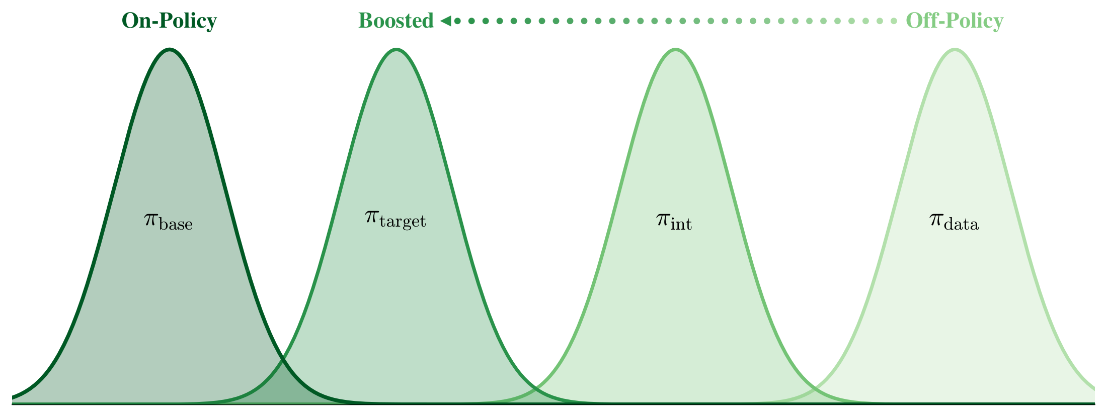
In this section, we present our sampling algorithm that maps off-policy expert data closer to the base model distribution for finetuning. Our procedure formalizes interpolating off-policy information into on-policy learning as highlighted in Section 1. To construct an informational-equivalent dataset that is easiest for the base model to internalize, we must provide a generation policy that maintains this information with minimal KL divergence. This specifies a target data generation distribution, and hence, all that remains is for us to explicitly provide an algorithm that samples from it.

The remainder of the section is organized as follows. Section 4.1 presents our formalization specifying this (unnormalized) boosted target data policy. Section 4.2 introduces a Markov chain Monte Carlo (MCMC) algorithm that approximately samples from this policy and ensures our sampling procedure produces generation policies that get progressively closer to the base model distribution. Finally, Section 4.3 outlines our implementation of this algorithm for LLMs.

4.1 Targeting the Information Projection

Suppose we are given a dataset of expert query-trajectory pairs

D={(qi,xi)}i=1N\mathcal{D} = \{(\mathbf{q}_{i}, \mathbf{x}_{i})\}_{i=1}^N

. For notational convenience, we fix a query

qi\mathbf{q}_i

for some

i

for the remainder of the section and assume all distributions are implicitly conditioned on

qi\mathbf{q}_{i}

. We can easily lift this assumption by stitching together the conditionals across

\leq i \leq N

For a given equivalence relation on trajectories, let

C\mathcal{C}

define the set of all trajectories

x∈X∗\mathbf{x}\in \mathcal{X}^*

that are equivalent to the associated expert trajectory

xi\mathbf{x}_{i}

. For theoretical purposes, we assume the existence of such an equivalence relation a priori; however, in practice,

C\mathcal{C}

refers to a task-dependent notion of ''correctness'' or ''semantic equivalence''. For example, for math/science reasoning, a semantically equivalent trajectory

x\mathbf{x}

refers to any trajectory leveraging information from expert trace

xi\mathbf{x}_{i}

that results in a correct final answer. For fact learning, a semantic equivalent

x\mathbf{x}

must contain the same factual content as

xi\mathbf{x}_{i}

, as judged by an automated (LLM) grader.

Definition

Let

PC\mathcal{P}_{\mathcal{C}}

denote the space of all distributions over token sequences

X∗\mathcal{X}^*

that have conditional support on

C\mathcal{C}

: that is, for a policy

π∈PC\pi \in \mathcal{P}_{\mathcal{C}}

, we have

π(x)=0\pi(\mathbf{x}) = 0

x∉C\mathbf{x} \notin \mathcal{C}

. In other words, informally,

PC\mathcal{P}_{\mathcal{C}}

is the set of all distributions that output only trajectories that are equivalent to the expert traces.

Our setup naturally admits a well-specified formalism for boosting off-policy data. The dataset of expert trajectories itself is drawn from some arbitrary policy

\in \mathcal{P}_{\mathcal{C}}

, implying the SFT objective Equation (2) minimizes the cross-entropy

Eq[−log⁡p]\mathbb{E}_q[- \log p]

. However, for arbitary

q

, this objective can be arbitarily off-policy. Given that we want to preserve the information signal of

D\mathcal{D}

with trajectories that are as on-policy as possible, this is equivalent to finding the distribution in

PC\mathcal{P}_{\mathcal{C}}

closest to the base model distribution

p

Definition 1

The information projection ([28]) of

p

onto

PC\mathcal{P}_{\mathcal{C}}

is defined as

Proposition

The distribution that uniquely minimizes the objective Equation (3) is the restriction of the base model onto equivalent trajectories:

where

1(x∈C)\mathbf{1}\bigl(\mathbf{x} \in \mathcal{C}\bigr)

takes the value

1

x∈C\mathbf{x} \in \mathcal{C}

and

0

otherwise.

Proof: Note that for any

π∈PC\pi \in \mathcal{P}_{\mathcal{C}}

we have that

\begin{aligned} \mathrm{KL}\!\left( \pi \,\middle\|\, p \right) &= \sum_{\mathbf{x}\in \mathcal{X}^*} \pi(\mathbf{x}) \log \frac{ \pi(\mathbf{x}) }{ p(\mathbf{x}) } = \sum_{\mathbf{x}\in \mathcal{C}} \pi(\mathbf{x}) \log \frac{ \pi(\mathbf{x}) }{ p(\mathbf{x}) }, \end{aligned}

since

π(x)=0\pi(\mathbf{x}) = 0

x∉C\mathbf{x} \notin \mathcal{C}

. Now

π\pi

defines a distribution over

x∈C\mathbf{x} \in \mathcal{C}

, but

p

is not normalized under the restriction to correct trajectories. However, we can rewrite

p(x)=Z⋅pC(x)p(\mathbf{x}) = Z \cdot p_{\mathcal{C}}(\mathbf{x})

for

x∈C\mathbf{x} \in \mathcal{C}

, where

\sum_{\mathbf{x}'\in \mathcal{C}} p(\mathbf{x}')

, so

p)\mathrm{KL}\!\left( \pi \,\middle\|\, p \right)

simplifies to

\sum_{\mathbf{x}\in \mathcal{C}} \pi(\mathbf{x}) \log \frac{ \pi(\mathbf{x}) }{ Z \cdot p_{\mathcal{C}}(\mathbf{x}) } =-\log Z + \sum_{\mathbf{x}\in \mathcal{C}} \pi(\mathbf{x}) \log \frac{ \pi(\mathbf{x}) }{ p_{\mathcal{C}}(\mathbf{x}) } = \mathrm{KL}\!\left( \pi \,\middle\|\, p_{\mathcal{C}} \right) -\log Z,

since

∑x∈Cπ(x)=1\sum_{\mathbf{x}\in \mathcal{C}} \pi(\mathbf{x}) = 1

and both

π\pi

and

pCp_{\mathcal{C}}

define a distribution over

C\mathcal{C}

. Then since

log⁡Z\log Z

is a constant independent of

π\pi

, it follows that the expression is uniquely minimized at

π=pC\pi = p_{\mathcal{C}}

, as desired.

The unnormalized projection

pC(x)∝p(x)⋅1(x∈C)p_{\mathcal{C}}(\mathbf{x}) \propto p(\mathbf{x}) \cdot \mathbf{1}\bigl(\mathbf{x} \in \mathcal{C}\bigr)

is thus our target distribution, as it is the closest distribution to the base model that also maintains the information content of the off-policy expert traces. Of course, if the base model

p

can reliably generate expert trajectories itself, the easiest way to sample from

pCp_{\mathcal{C}}

is to simply perform rejection sampling, which already lends itself to a rudimentary form of on-policy RL ([11]).

However, we are interested in the regime where rejection sampling is infeasible, and the expert trajectories are difficult to attain via the base model alone. Then our task is now the following: given access to an arbitrary initial expert policy

q

via dataset trajectories, can we algorithmically evolve samples from

q

into informational-equivalent but more on-policy samples from

pCp_{\mathcal{C}}

4.2 The Metropolis-Hastings Algorithm

We indeed can, by appealing to Markov Chain Monte Carlo (MCMC) approximate sampling techniques. Specifically, we will use a Metropolis-Hastings (MH) sampler ([29, 30]), which constructs a Markov chain of sample sequences

(x0,x1,…,xn)(\mathbf{x}^0, \mathbf{x}^1, \dots, \mathbf{x}^n)

using a proposal distribution

κ(x∣xi)\kappa(\mathbf{x}|\mathbf{x}^i)

to select the next candidate

xi+1\mathbf{x}^{i+1}

. With probability

candidate

x\mathbf{x}

is accepted as

xi+1\mathbf{x}^{i+1}

; otherwise, MH sets

xi+1=xi\mathbf{x}^{i+1} = \mathbf{x}^{i}

. It is a classic fact that as

\to \infty

, this process converges to sampling from the target distribution

pCp_{\mathcal{C}}

, provided that the Markov chain satisfies the following properties:

Definition

The proposal distribution

κ\kappa

is irreducible if under the induced Markov chain, for any states

x,x′\mathbf{x},\mathbf{x}'

with nonzero mass under the target distribution

pCp_{\mathcal{C}}

, the probability of transitioning to

x′\mathbf{x}'

starting from

x\mathbf{x}

after some number of steps is nonzero. The proposal is aperiodic if the induced chain of samples does not return to the same sample after a fixed interval number of steps.

Since we are given a dataset of expert traces, we would like to initialize the Markov chain with such a trace and restrict our attention to proposal distributions

κC\kappa_{\mathcal{C}}

that ensure that

xi∈C\mathbf{x}^i \in \mathcal{C}

for all

i

. We refer to such proposal distributions as information-preserving.

Although this might seem to violate the irreducibility criterion, notice we can rewrite Equation (5) as the following:

A(\mathbf{x}, \mathbf{x}^i) = \text{min} \left\lbrace 1, \frac{p(\mathbf{x}) \cdot \kappa(\mathbf{x}^i | \mathbf{x}) \cdot \mathbf{1}\bigl(\mathbf{x} \in \mathcal{C}\bigr)}{p(\mathbf{x}^i) \cdot \kappa(\mathbf{x}|\mathbf{x}^i) \cdot \mathbf{1}\bigl(\mathbf{x}^i \in \mathcal{C}\bigr)}\right\rbrace = \text{min} \left\lbrace 1, \frac{p(\mathbf{x}) \cdot \kappa_{\mathcal{C}}(\mathbf{x}^i | \mathbf{x})}{p(\mathbf{x}^i) \cdot \kappa_{\mathcal{C}}(\mathbf{x}|\mathbf{x}^i)}\right\rbrace.

Assuming current candidate

xi∈C\mathbf{x}^i \in \mathcal{C}

, if the new candidate

x∉C\mathbf{x} \notin \mathcal{C}

, the acceptance ratio defaults to

0

. In particular:

Proposition

Running Metropolis-Hastings with irreducible proposals

κ\kappa

and target distribution

pCp_{\mathcal{C}}

is equivalent to running MH with information-preserving proposals

κC\kappa_{\mathcal{C}}

and target distribution

p

This gives us a convenient recipe for boosting an off-policy dataset: initialize at the expert trajectory, mutate the candidates with some information-preserving proposal distribution

κC\kappa_{\mathcal{C}}

, and use Equation (6) to accept or reject candidates. In fact, not only does this process eventually converge to

pCp_{\mathcal{C}}

, but it also guarantees a progressive decrease in the policy gap between the data generation policy and the base model.

Proposition 2

For all

\geq 0

, let

πk\pi_k

denote the distribution over candidates obtained after

k

MCMC steps applied to initial expert policy

q

. Then we have

Proof: Let

Ψ\Psi

denote the MCMC transition kernel; i.e., the transformation induced by applying one step of our Metropolis-Hastings procedure.

Ψ\Psi

has stationary distribution

pCp_{\mathcal{C}}

, so

Ψ(pC)=pC\Psi(p_{\mathcal{C}}) = p_{\mathcal{C}}

. Since

Ψ\Psi

is Markovian, it follows from the data processing inequality that

Now, for any

π\pi

, recall from Equation (4) that

p)+log⁡Z\mathrm{KL}\!\left( \pi \,\middle\|\, p_{\mathcal{C}} \right) = \mathrm{KL}\!\left( \pi \,\middle\|\, p \right) + \log Z

for some fixed constant

Z

, so it follows that

p)\mathrm{KL}\!\left( \pi_{k+1} \,\middle\|\, p \right) \leq \mathrm{KL}\!\left( \pi_k \,\middle\|\, p \right)

, as claimed.

In other words, the Metropolis-Hastings procedure progressively shifts the original expert policy to informational-equivalent policies that get progressively closer to the base model distribution.

4.3 Projection Sampling for LLMs

As detailed in [22], a direct implementation of Metropolis-Hastings for LLMs is infeasible as it requires regenerating full-length token sequences with repeated LLM inference calls. This infeasibility is further compounded by slow mixing, where convergence can require exponentially many MCMC steps due to high dimensional sample spaces or poor choice of proposals and initializations.

To help avoid these issues, we adapt the implementation of Metropolis-Hastings for power sampling in [22], which we refer the reader to for further details. In short, we define restriction distributions of the target projection

pCp_{\mathcal{C}}

over sequences of increasing length in units of block size

B

. We use Metropolis-Hastings to sample within each distribution, providing a strong initialization to begin sampling from the next one. The full details are presented in Algorithm 1.

Algorithm 1: Projection Sampling with Autoregressive Models

Input: base ppp; proposal κC\kappa_{\mathcal{C}}κC​; expert trajectory τ\tauτ; length TTT
Hyperparams: block size BBB; MCMC steps NMCMCN_{\mathrm{MCMC}}NMCMC​
Output: (x0,…,xT)∼pC(x_0,\dots,x_T) \sim p_{\mathcal{C}}(x0​,…,xT​)∼pC​
Notation: Define the unnormalized intermediate target
πk(x0:kB)  ∝  pC(x0:kB).{\pi}_k(x_{0:kB}) \;\propto\; p_{\mathcal{C}}(x_{0:kB}).πk​(x0:kB​)∝pC​(x0:kB​).
for k←0k \gets 0k←0 to ⌈TB⌉−1\lceil \frac{T}{B}\rceil-1⌈BT​⌉−1:
  Given prefix x0:kBx_{0:kB}x0:kB​, we wish to sample from πk+1\pi_{k+1}πk+1​. Construct initialization x0{\mathbf{x}}^{0}x0 by extending autoregressively with κC\kappa_{\mathcal{C}}κC​:
  xt(0)∼κC(xt∣x<t,τ),for kB+1≤t≤(k+1)B.x^{(0)}_t \sim \kappa_{\mathcal{C}}\big(x_t \mid x_{<t}, \tau\big), \qquad\text{for } kB+1 \leq t \leq (k+1)B.xt(0)​∼κC​(xt​∣x<t​,τ),for kB+1≤t≤(k+1)B.
  Set the current state x←x0\mathbf{x} \gets \mathbf{x}^{0}x←x0.
  for n←1n \gets 1n←1 to NMCMCN_{\mathrm{MCMC}}NMCMC​:
    Sample an index m∈{1,…,(k+1)B}m \in \{1,\dots, (k+1)B\}m∈{1,…,(k+1)B} uniformly.
    Construct proposal sequence x′\mathbf{x}'x′ with prefix x0:m−1x_{0:m-1}x0:m−1​ and resampled completion:
    xt′∼κC(xt∣x<t,τ),for m≤t≤(k+1)B.x'_{t} \sim \kappa_{\mathcal{C}}\big(x_t \mid x_{<t}, \tau\big), \qquad\text{for } m \leq t \leq (k+1)B.xt′​∼κC​(xt​∣x<t​,τ),for m≤t≤(k+1)B.
    Compute acceptance ratio Equation (5)
    A(x′,x)  ←  min⁡{1, p(x′)p(x)⋅κC(x∣x′,τ)κC(x′∣x,τ)}.A(\mathbf{x'}, \mathbf{x}) \;\gets\; \min\Bigg\{1,\ \frac{p(\mathbf{x'})}{p(\mathbf{x})} \cdot \frac{\kappa_{\mathcal{C}}(\mathbf{x}\mid \mathbf{x'}, \tau)}{\kappa_{\mathcal{C}}(\mathbf{x'}\mid \mathbf{x}, \mathbf{\tau})} \Bigg\}.A(x′,x)←min{1, p(x)p(x′)​⋅κC​(x′∣x,τ)κC​(x∣x′,τ)​}.
    Draw u∼Uniform(0,1)u \sim \mathrm{Uniform}(0,1)u∼Uniform(0,1);
    if u≤A(x′,x)u \le A(\mathbf{x'}, \mathbf{x})u≤A(x′,x): accept and set x←x′\mathbf{x} \gets \mathbf{x'}x←x′
  Set x0:(k+1)B←xx_{0:(k+1)B} \gets \mathbf{x}x0:(k+1)B​←x to fix the new prefix sequence for the next stage.
return x0:Tx_{0:T}x0:T​

It remains to define an appropriate proposal distribution, as this crucial object facilitates information-preservation and is the only component of Algorithm 1 that interacts with the expert trajectory.

To craft our choice of

κC\kappa_{\mathcal{C}}

, we use a trick also utilized in [12, 13] which leverages the strong in-context instruction-following capabilities of pretrained LLMs. Suppose we are given candidate

x=(x0,⋯xL)\mathbf{x} = (x_0, \cdots x_L)

. Our proposal distribution uniformly at random selects an index

\in [1, L]

and creates a partial trace by truncating the suffix after

t

,xt)\tilde{\mathbf{x}} = (x_0, \cdots, x_t)

. Then, we pass this partial trace along with the expert trajectory

τ\tau

in-context to a simple prompt template similar to ones used in [12]:

You are given a question, an expert solution, and an initial, partial response. Examine the solution, identifying all information provided in the reasoning process. 

Question: <QUERY>

This is an expert solution to the query: <TRAJECTORY>

Here is a partial response: <PARTIAL TRACE>

Starting with the partial response, continue in your own words, including the thinking process. Ensure your response is logically consistent with the expert solution and leads to a complete and correct final answer.

Then our proposal

κC\kappa_{\mathcal{C}}

is simply the distribution defined by conditioning our base model

p

on this prompt. In practice, we find that this prompt can sufficiently generate correct trajectories from expert demonstrations, satisfying the constraint of information-preservation.

With this final piece specified, to construct our boosted dataset for finetuning, we simply apply Algorithm 1 to each query-trajectory pair in our expert dataset

D\mathcal{D}

. For examples of boosted traces across different models and datasets, see Appendix A.

Since our Metropolis-Hastings procedure targets sampling from the information projection given information constraints

C\mathcal{C}

, we refer to our sampling algorithm as projection sampling.

Unlike in [22], where the sampling algorithm incurs an inference-time cost, projection sampling only incurs a one-time cost, as it is conducted on the training dataset prior to finetuning. To quantify this cost, we can estimate the average number of tokens expended by Algorithm 1. For each trajectory

τ∈D\tau \in \mathcal{D}

, each MCMC step resamples an average of

kB2\frac{kB}{2}

tokens, carried out

NMCMCN_{\text{MCMC}}

times. Summing, we have

We can lower the cost by increasing the block size

B

, but in general, since projection sampling is a fixed cost, we prefer smaller block sizes that provide higher resolution and less approximation error.

5. Experiments

We now empirically demonstrate that the trajectories generated by our sampling algorithm enable SFT to break its weak characterization, frequently outperforming existing on-policy learning algorithms for posttraining.

5.1 Experimental Setup

Tasks. We select a set of learning tasks that are characteristic of the range of capabilities posttraining seeks to introduce, including novel skill acquisition, reasoning, and open-ended expertise. In the following discussion, we present three tasks. Each learning task is accompanied by expert trajectories which are either inherent to the dataset or generated by GPT-5.

Chemistry: We examine whether a pretrained LLM can pick up a new set of skills that it is not explicitly finetuned on beforehand. Following [13], we take scientific reasoning as the test domain. In this setting, we use Chemistry L-3 subset of SciKnowEval ([31]) that includes skills like reaction prediction, molar weight calculation, and chemical equation balancing. Moreover, some questions follow a multiple choice format, while others (balancing) are freeform, representing a mixed dataset with a harder-to-specify reward for on-policy RL. There are 2400 problems total, with 1800 training problems and 600 test problems. Expert trajectories are generated by GPT-5.
Math: We investigate whether a pretrained LLM with some general mathematical ability can improve performance on a set of hard math reasoning problems relative to the base model. In this setting, we use the MATH ([3]) dataset restricted to the hardest problem classes: Levels 3, 4, and 5. There are 9254 problems total, with 8230 training problems and 1024 test problems that are accompanied by existing expert solutions.
Medical: We test whether our approach is effective in more open-ended domains that are not as immediately verifiable as the prior two. As in [13], we look at medical question answering. We use the HuatuoGPT-o1 SFT dataset ([32]), which provides 19704 questions requiring clinical reasoning skills for diagnoses, treatments, and general medical knowledge, and each question has a provided expert response. For evaluation, we select 1000 questions uniformly at random from the HuatuoGPT-o1 RL dataset that are never seen during training.

Models. For the given posttraining tasks, we select base models across varying model families and sizes that are not already proficient or finetuned on the task domains. For chemistry, we use Qwen2.5-7B-Instruct ([33]) and Olmo-3-7B-Instruct ([34]), which achieve test set accuracies

34.3%34.3\%

and

32.8%32.8\%

respectively. For math, we use Qwen2.5-3B, which achieves test accuracy

31.5%31.5\%

. Finally, for medical, we use Qwen2.5-7B-Instruct, which achieves test accuracy

35.3%35.3\%

Evaluation. We include several benchmarks for each task that holistically measure both task-specific generalization and retention of prior capabilities. All benchmarks are scored based on single-shot accuracy.

Chemistry: We measure generalization capabilities in domain with the test set for SciKnowEval. To measure prior capabilities, we evaluate on math benchmarks AMC, MATH500, and GSM8K ([35]) alongside MMLU ([36]) and GPQA ([5]).
Math: To measure generalization capabilities, we track performance on the test set MATH(3,4,5) as well as out-of-distribution generalization on AMC, MATH500, and GSM8K. To track prior capabilities, we evaluate on MMLU, Chemistry, and GPQA.
Medical: Since medical reasoning is a more open-ended domain, we use an automated LLM grader (GPT-5-mini) to evaluate correctness on the test set (see Appendix C.3 for the exact grading prompt). For capability retention, we evaluate AMC, MATH500, GSM8K, MMLU, and GPQA.

Baselines. For each task, we benchmark against a wide variety of posttraining algorithms ranging from vanilla SFT to on-policy learning with privileged information via RL and self-distillation.

Chemistry: We compare our method on all evaluations for this task to the base models, SFT with the expert dataset trajectories, and a variant of SFT using our sampling proposal prompt to rewrite each expert trajectory; i.e., " $0th0^{\text{th}}$ order MCMC". In addition, we include on-policy self-distillation (OPSD) ([13, 18]), which distills from the base model conditioned on privileged information.
Math: We use the baselines used in chemistry alongside two RL baselines, since the rollouts are easily verifiable. We include GRPO ([37]) as well as a stronger variant UFT ([14]), which uses the off-policy expert traces as privileged information during rollout generation.
Medical: Same baselines as chemistry.

Sampling. For all datasets, we use block number

B = 32

with maximum sequence length

T = 1856

over

NMCMC=10N_{\text{MCMC}} = 10

MCMC steps.

Training. For all tasks, all SFT training runs are tuned with the following hyperparameters across the corresponding ranges: epoch number:

{1, 2\}

, learning rate:

{\{

5e-5, 1e-5, 5e-6

}\}

, and batch size:

{16, 32, 64\}

. For the medical task, we extend the epoch range to

{1, 2, 4, 6\}

to accommodate a larger dataset. The optimizer is AdamW with a cosine scheduler and gradient clipping for norms greater than

1

. The on-policy self-distillation runs are tuned with hyperparameters from ([13]) while the RL baselines use the default hyperparameters from ([14]). All models are trained using H100s and H200s.

5.2 Main Results

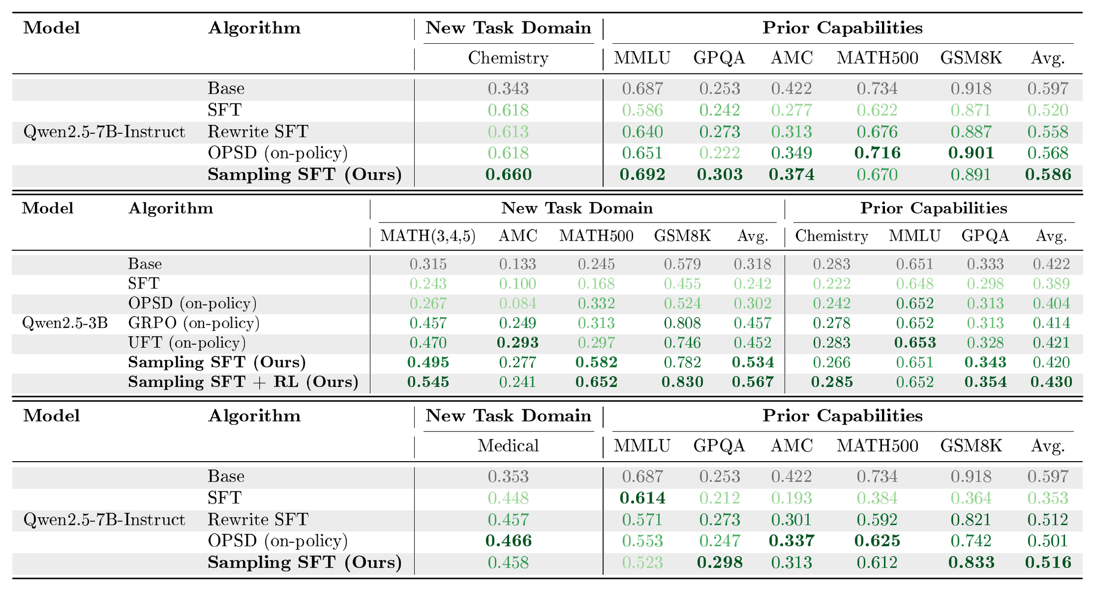
Table 1: Sampling enables SFT to generalize better while forgetting less. Top: Chemistry on Qwen2.5-7B-Instruct. Middle: Math on Qwen2.5-3B. Bottom: Medical on Qwen2.5-7B-Instruct. We bold the highest score in each column, and for math, we also bold if one of our listed approaches outperforms the other baselines, with a color gradient to emphasize numerical gaps. Across model sizes and evaluation tasks, sampling consistently enables SFT to generalize and retain prior capabilities at least as well as, if not better than, its on-policy posttraining counterparts.

We display our main results for the Qwen model family in Table 1. For results on Olmo, see Section 5.3 and Appendix B.

Stronger generalization. Across different pretrained base models and different tasks, we see that projection sampling enables SFT to achieve an exceptionally strong performance when evaluated on new capabilities introduced in finetuning. In chemistry, sampling SFT is able to improve base model performance on chemistry by +31.7%, exceeding even the improvement yielded by the on-policy OPSD by +4.20%. Simple zero-shot rewrites of the off-policy traces do not perform as strongly in this setting, suggesting the importance of the full MCMC process in Algorithm 1.

Math reasoning vividly illustrates that capability gains transfer to adjacent out-of-distribution test domains as well. Whereas vanilla SFT leads to a drop in performance across the board in math benchmarks, sampling SFT yields a +18.0% boost on the hardest problems in the MATH benchmark, even surpassing the reasoning boosts obtained by GRPO and UFT. This extends to a +14.4% boost on AMC and a +20.3% boost on GSM8K, which are on par with the boosts obtained by either RL algorithm. The performance gain on MATH500 is especially notable, providing a +33.7% boost to the base model and surpassing the next best performing (RL) baseline by +26.9%.

Not only does the sampling SFT model generalize well, but it also provides a strong initialization for RL that leads to even further gains. In the math section of Table 1, we record GRPO initialized with the sampling SFT checkpoint (Sampling SFT-RL) and observe that it is the strongest performing model overall, achieving +40.7% performance in MATH500 and +25.1% performance in GSM8K: within reach of the 7B-Instruct model.

With just off-policy expert traces, SFT can fail to generalize well. But composed with our sampling algorithm, SFT can exhibit exceptionally strong generalization, even outperforming RL and OPSD baselines. The fact that this sampling procedure is custom to the base model distribution is crucial: Appendix B details results demonstrating that finetuning, e.g., Qwen on the same base task data but boosted for Olmo severely underperforms all baselines.

Retaining prior capabilities. This strong generalization does not come at the cost of catastrophic forgetting. For chemistry in Table 1, vanilla SFT results in a considerable drop in capabilities. Meanwhile, sampling SFT does not lose any MMLU knowledge and reduces the average loss in prior task accuracy down to just -1.10%. In fact, our model forgets the least, even including OPSD. These results are mirrored in the medical domain, where sampling recovers a 16.3% loss in average prior capabilities with vanilla SFT, and again, forgets the least among all baselines.

5.3 Analysis

We now examine distributional properties of our sampled traces for finetuning as well as those of the resulting model capabilities.

Dataset likelihoods. We can directly observe the effect projection sampling has on expert traces.

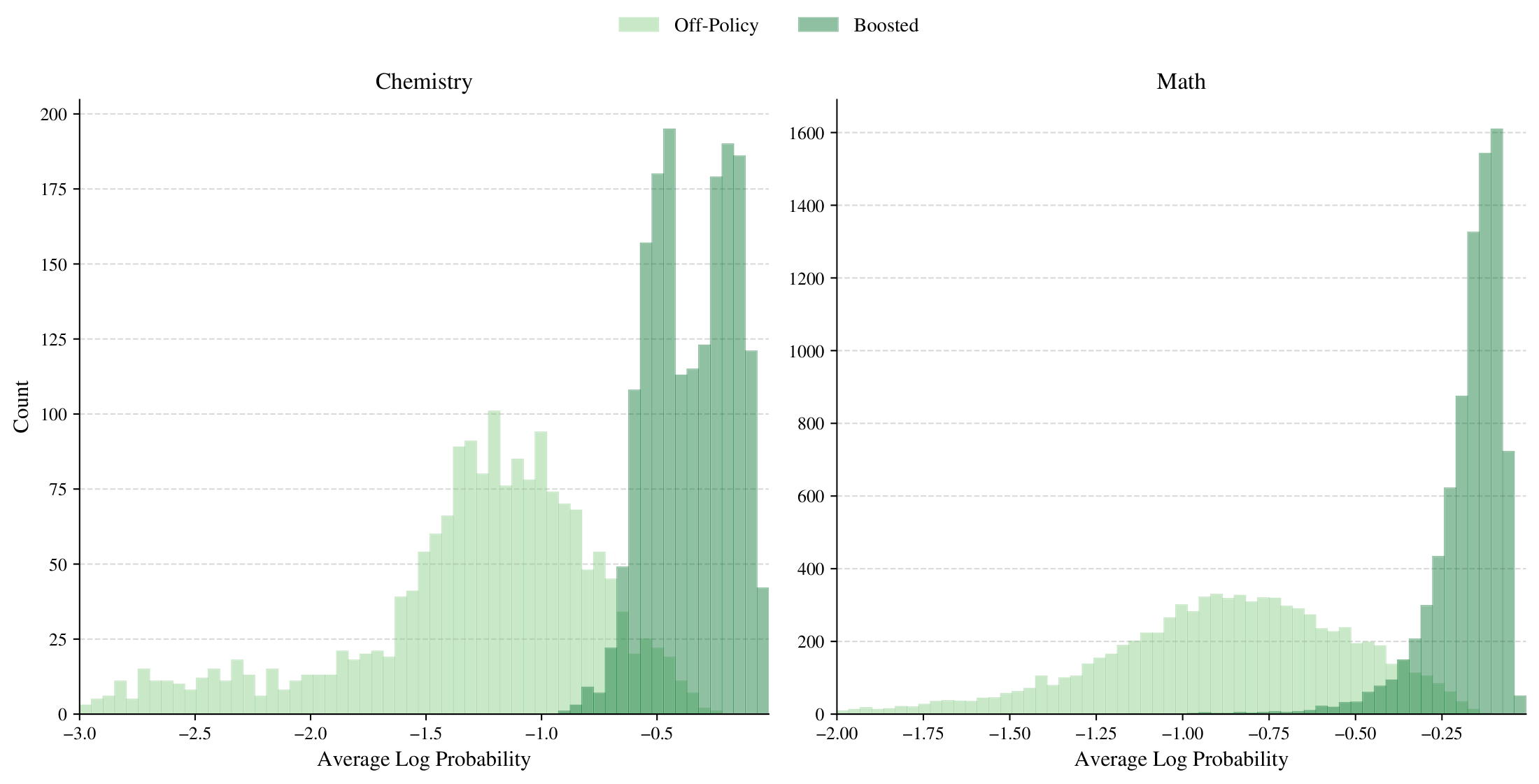
Figure 3 plots histograms of the sequence log-likelihoods (averaged by length) under the base model of both the expert traces and the boosted traces for both science and math reasoning. The on-policy projection is apparent, yielding traces that are much higher-likelihood relative to the base model while preserving correctness.

Learning beyond sharpening. In Section 1, we highlighted the overarching goal of posttraining as introducing fundamentally new capabilities that are not present in the base model. Given that projection sampling pushes off-policy data to be more in-distribution, can our finetuned models still acquire new behaviors beyond just sharpening existing ones?

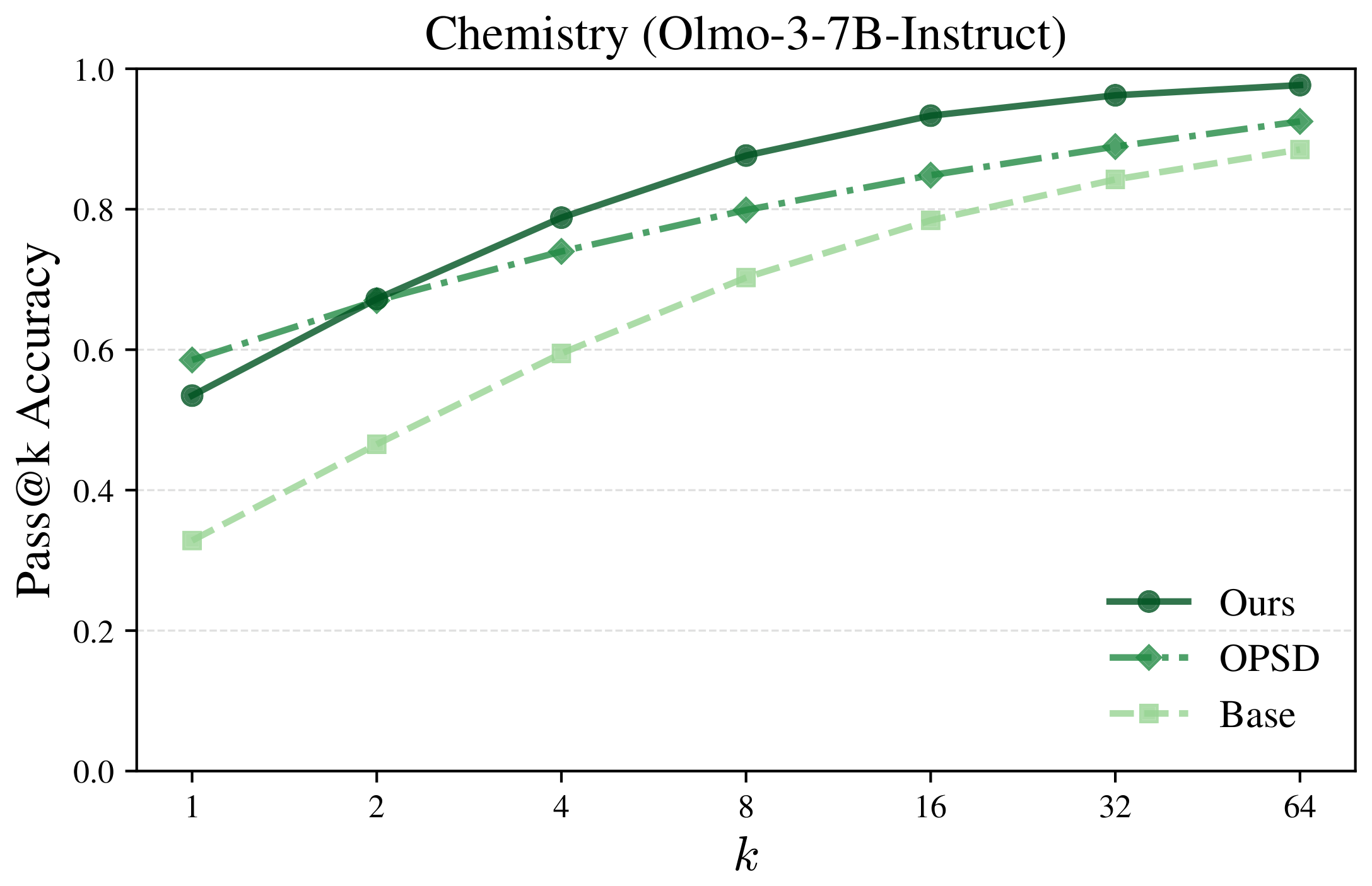
We answer in the affirmative. In Figure 4, we examine the pass@

k

accuracy of Olmo-3-7B-Instruct relative to finetuning with sampling (ours) as well as on-policy distillation with privileged information (OPSD) on the science task. If finetuning with our sampling algorithm was simply sharpening existing capabilities, we would expect our pass@

k

curve to eventually converge to the base model. However, we actually see large, consistent gaps in the pass@

k

rate up to very large

k

, demonstrating that our finetuned model has fundamentally stronger capabilities than the base model. Moreover, for

k > 2

, we see substantial gaps in our pass@

k

rate relative to OPSD, indicating that our method enables learning capabilities that OPSD does not learn.

We can also be more granular at the the level of individual evaluation problems. In other words, we can identify "hard problems" that the base model absolutely cannot solve (pass@

k

rate zero for highest

k

) but our finetuned model can start reliably solving: in fact, some evaluation tasks go from zero pass rate in the base model to pass rates that are up to 67.2% or 53.1%.

Scaling sampling compute. Proposition 2 observes that increasing the number of MCMC steps in projection sampling results in data generation policies

πk\pi_k

that are progressively closer to the base model in KL divergence. This frames sampling as a natural axis for scaling compute, expending more MCMC steps for more on-policy learning data.

We can directly observe this scaling empirically in Figure 5. For base model Qwen2.5-7B-Instruct on the science task, we apply

k

MCMC steps to the off-policy training data, for

\in [0, 2, 4, 6, 8, 10]

. Note that

k = 0

corresponds to a data rewrite, i.e., asking the base model to simply rewrite off-policy data "in its own words". On the left vertical axis, we plot

πbase)\mathrm{KL}\!\left(\pi_{k}\,\middle\|\,\pi_{\text{base}}\right)

, where

πk\pi_k

is the data generation policy induced by

k

MCMC steps. We can directly estimate this KL divergence as trajectories are repeatedly generated by a proposal distribution (

κC(⋅∣τ)\kappa_{\mathcal{C}}( \cdot | \tau)

in Algorithm 1) parametrized by an LLM, from which we can extract next-token log probabilities. On the right vertical axis, we plot the accuracy of the base model finetuned on the boosted data for each

k

. As we increase sampling compute, the boosted data distribution monotonically closes the KL gap with the base model, while the corresponding finetuned models trend upwards in accuracy. Hence, empirically, more MCMC steps lead to more on-policy data, which results in better generalization after finetuning.

6. Conclusion

In this work, we introduce a formalism that bridges an apparent disconnect between privileged off-policy information and on-policy training. By carefully boosting the likelihood of off‑policy expert data towards the base model’s distribution, we obtain a more on‑policy equivalent that is far more suitable for learning. Indeed, across science, math reasoning, and open-ended expertise, SFT on boosted data can generalize better and forget less than both vanilla SFT and strong on‑policy baselines, including RL and self‑distillation. The resulting models also exhibit strong distributional performance over multiple samples and are able to learn fundamentally new capabilities that are not present in the base model.

Beyond just SFT, sampling offers a powerful framework for the posttraining stack, acting as a model-native operator that shapes data for learnability. For example, for on-policy distillation, our MCMC process directly induces a teacher distribution from initial distillation traces that is much closer in KL divergence to the student, facilitating more stable updates. Likewise, conditioned on expert information, our method can simulate on-policy rollouts for RL on hard tasks where the base model is unable to generate signal. By expending sampling-time compute in exchange for stronger, more on-policy trace distributions constructed from privileged information, sampling provides a simple, robust, and scalable pathway for continually expanding LLM capabilities.

7. Acknowledgements

A.K. would like to thank the Paul and Daisy Soros Foundation, NDSEG Fellowship, and Kempner Institute for their support. S.C. was supported in part by NSF CAREER award CCF-2441635 and the Harvard Dean's Competitive Fund for Promising Scholarship.

Appendix

A. Examples of Boosted Off-Policy Data

Chemistry (Olmo-3-7B-Instruct)

Question: Given a chemical equation, please balance the equation and maintain the order of reactants and products as given. Here is an unbalanced chemical equation:

Explain your reasoning, thinking step by step, and return the balanced equation on one line. Keep reactants and products in the SAME ORDER as provided.

Original: To balance the given chemical equation, we need to ensure the number of atoms of each element is equal on both sides of the equation. Starting with carbon (C), there is 1 atom of C in CO

_2

on the reactant side, but 3 atoms in C

_3

_6

_3

on the product side. To balance the carbon atoms, we need 3 CO

_2

molecules. Next, balance the hydrogen (H) atoms. There are 2 H atoms in each H

_2

O molecule and 6 H atoms in C

_3

_6

_3

. Therefore, we need 3 H

_2

O molecules. Now, balance the oxygen (O) atoms. We have a total of

\times 2 = 6

O from CO

_2

and

\times 1 = 3

O from H

_2

O, amounting to 9 O atoms on the reactant side. On the product side, C

_3

_6

_3

contributes 3 O atoms, leaving 6 O atoms needed for O

_2

. Since one O

_2

molecule contains 2 O atoms, 3 O

_2

molecules are required. The balanced equation is:

Boosted: Looking at the given equation, CO

_2

+ H

_2

→\rightarrow

_3

_6

_3

+ O

_2

, the first step is to identify the number of atoms of each element on both sides. For carbon, there is 1 C per CO

_2

molecule on the left, but 3 C atoms in C

_3

_6

_3

on the right, so we must place a coefficient of 3 in front of CO

_2

to balance carbon. This gives us 3 CO

_2

on the left. Next, we check hydrogen: the right side has 6 H atoms in C

_3

_6

_3

, while each H

_2

O provides 2 H atoms. So we need 3 H

_2

O molecules (since

\times 2 = 6

H). Now, for oxygen: on the left, 3 CO

_2

gives 6 O atoms and 3 H

_2

O gives 3 O atoms, totaling 9 O atoms. On the right, C

_3

_6

_3

contains 3 O atoms, so the remaining 6 O atoms must come from O

_2

(since each O

_2

molecule has 2 O atoms, we need 3 O

_2

molecules to provide 6 O atoms). Thus, the balanced equation is:

Math (Qwen2.5-3B)

Question: Rationalize the denominator of

1+31−3\frac{1+\sqrt{3}}{1-\sqrt{3}}

When you write your answer in the form

A+BCA+B\sqrt{C}

, where

A

B

, and

C

are integers, what is

A B C

? Explain your reasoning, thinking step by step, and return your final answer within <code>\boxed{}</code>.

Original: When we multiply both the numerator and denominator by the conjugate of the denominator, we get

1+31−3=(1+3)(1+3)(1−3)(1+3)\frac{1+\sqrt{3}}{1-\sqrt{3}} = \frac{(1+\sqrt{3})(1+\sqrt{3})}{(1-\sqrt{3})(1+\sqrt{3})}

Simplifying, we obtain

1+23+31−3=4+23−2=−2−3\frac{1+2\sqrt{3}+3}{1-3} = \frac{4+2\sqrt{3}}{-2} = -2-\sqrt{3}

Thus

A = - 2

B = - 1

C = 3

, and

ABC=6ABC=\boxed{6}

Boosted: To rationalize the denominator of

1+31−3\frac{1+\sqrt{3}}{1-\sqrt{3}}

, we need to multiply both the numerator and denominator by the conjugate of the denominator, which is

1+31+\sqrt{3}

Thus, in the form

A+BCA+B\sqrt{C}

, we have

A = - 2

B = - 1

, and

C = 3

Therefore,

ABC=(−2)(−1)(3)=6ABC=(-2)(-1)(3)=\boxed{6}

Medical (Qwen2.5-7B-Instruct)

Question: Given the symptoms of sudden weakness in the left arm and leg, recent long-distance travel, and the presence of swollen and tender right lower leg, what specific cardiac abnormality is most likely to be found upon further evaluation that could explain these findings?

Original: The specific cardiac abnormality most likely to be found in this scenario is a patent foramen ovale (PFO). This condition could allow a blood clot from the venous system, such as one from a deep vein thrombosis in the leg, to bypass the lungs and pass directly into the arterial circulation. This can occur when the clot moves from the right atrium to the left atrium through the PFO. Once in the arterial system, the clot can travel to the brain, potentially causing an embolic stroke, which would explain the sudden weakness in the left arm and leg. The connection between the recent travel, which increases the risk of deep vein thrombosis, and the neurological symptoms suggests the presence of a PFO facilitating a paradoxical embolism.

Boosted: Given the patient's history of recent long-distance travel, there is an increased risk of developing a deep vein thrombosis (DVT) due to prolonged immobility during the flight. This DVT, if it occurs in the right lower leg, can lead to swelling and tenderness in that area. Additionally, the presence of a patent foramen ovale (PFO) allows for a potential mechanism by which a clot from the DVT might bypass the pulmonary circulation and travel to the left side of the heart. From there, the clot could enter the systemic circulation and potentially cause an embolic event in the brain, leading to the sudden weakness in the left arm and leg. Therefore, upon further evaluation, the most likely finding would be:

A patent foramen ovale (PFO), which facilitates the passage of a clot from the right side of the heart to the left side, allowing it to reach the cerebral circulation and cause a stroke-like presentation.

Math (Qwen2.5-3B)

Question: You are an expert mathematician. Can you solve the following math problem? Suppose that

h(x)=f^{-1}(x)

. If

h (2) = 10

h (10) = 1

and

h (1) = 2

, what is

f (f (10))

? Explain your reasoning, thinking step by step, and return your final answer within <code>\boxed{}</code>.

Original: Since

f

and

h

are inverse functions and

h (2) = 10

f (10) = 2

, so

f (f (10)) = f (2)

. And since

h (1) = 2

\boxed{1}

Boosted: To find

f (f (10))

, we can use the information given about the function

h(x) = f^{-1}(x)

. Since

h (2) = 10

, it means that

f (10) = 2

. Similarly, since

h (1) = 2

, it implies that

f (2) = 1

. Therefore,

\boxed{1}

Medical (Qwen2.5-7B-Instruct)

Question: A 4-year-old boy is brought to the emergency department with a morbilliform rash, fever, cracked lips, cervical lymphadenopathy, and desquamation of the perianal region, suggesting a condition that can lead to serious complications. Which anatomical structure is most critical to evaluate for potential complications in this clinical scenario?

Original: In this clinical scenario, the symptoms presented by the 4-year-old boy suggest Kawasaki disease, a condition especially relevant for its potential complications involving the heart. Most critically, the anatomical structures to evaluate in this case are the coronary arteries. This is because one of the severe complications of Kawasaki disease is the development of coronary artery aneurysms, which can lead to significant cardiac issues. Regular monitoring through echocardiography is often employed to assess the condition of the coronary arteries and ensure timely intervention if needed.

Boosted: Based on the clinical presentation, the patient's symptoms strongly suggest Kawasaki disease. Given the symptoms such as a morbilliform rash, fever, cracked lips, cervical lymphadenopathy, and desquamation of the perianal region, it is crucial to focus on evaluating the cardiovascular system for potential complications. The coronary arteries are the most critical anatomical structures to assess in this case. This is due to the high risk of developing coronary artery aneurysms, which can occur in up to 25% of untreated cases. These aneurysms can lead to serious cardiac issues such as myocardial infarction or sudden cardiac death. Therefore, regular echocardiographic monitoring is essential to detect any abnormalities early and provide timely intervention if necessary. In summary, the coronary arteries should be the primary focus when assessing this patient to prevent life-threatening complications associated with Kawasaki disease.

Chemistry (Qwen2.5-7B-Instruct)

Question: Given a question and four options, think step by step, and then return the correct letter: A, B, C, or D. The last line of your response should be of the following format:

LETTER\boxed{{\text{{LETTER}}}}

, where LETTER is one of ABCD (ex.

A\boxed{{A}}

What is the molar weight (g/mol) of the molecule with the the IUPAC name '(2R, 3R, 4S, 5S)-oxane-2,3,4,5-tetrol'?

Options:

A) 148.160
B) 150.130
C) 151.140
D) 149.150

Explain your reasoning, thinking step by step, and return your final answer within <code>\boxed{}</code>.

Original: To find the molar weight of the molecule '(2R, 3R, 4S, 5S)-oxane-2,3,4,5-tetrol', we first need to determine its molecular formula. The name suggests that it is a tetrahydroxy derivative of oxane, which is a cyclic ether with six atoms (similar in structure to pyran). Since oxane can be considered as tetrahydropyran (with the chemical formula C5H10O), the molecule '(2R, 3R, 4S, 5S)-oxane-2,3,4,5-tetrol' would have four hydroxyl groups (-OH) attached to it. Therefore, the molecular formula would be C5H10O5:

Carbon (C): 5 atoms × 12.01 g/mol = 60.05 g/mol
Hydrogen (H): 10 atoms × 1.008 g/mol = 10.08 g/mol
Oxygen (O): 5 atoms × 16.00 g/mol = 80.00 g/mol

Adding these together gives us the molar weight:

Therefore, the molar weight of the molecule is 150.130 g/mol.

B\boxed{{B}}

Boosted: Starting with the IUPAC name '(2R, 3R, 4S, 5S)-oxane-2,3,4,5-tetrol', we can deduce the structure of the molecule. Oxane, also known as tetrahydropyran, has the structure of a five-membered ring containing one oxygen atom. The term "tetrol" indicates that this molecule has four hydroxyl (-OH) groups attached to the ring. Therefore, the molecular formula of this compound will be C5H10O5.

Let's break down the calculation of the molar weight step by step:

Carbon (C): There are 5 carbon atoms in the molecule. The atomic weight of carbon is approximately 12.01 g/mol.

Hydrogen (H): There are 10 hydrogen atoms in the molecule. The atomic weight of hydrogen is approximately 1.008 g/mol.

Oxygen (O): There are 5 oxygen atoms in the molecule. The atomic weight of oxygen is approximately 16.00 g/mol.

Adding these together gives us the molar weight of the molecule:

Therefore, the molar weight of the molecule is 150.130 g/mol.

B\boxed{{B}}

B. Additional Results

We include results on a non-Qwen-family model to demonstrate that our method applies to a variety of pretrained model families. Namely, we provide results for Olmo-3-7B-Instruct on the chemistry task.

We also include two more comparative experiments for the Chemistry task for Qwen2.5-7B-Instruct to stress that the alignment between data distribution and learning distribution is crucial. For the first, we take the boosted dataset relative to Olmo-3-7B and finetune Qwen2.5-7B-Instruct on that. We find the accuracy on Chemistry drops to 57.33%, which is significantly worse than the other baselines (61.8% for vanilla SFT). For the second experiment, we train Qwen2.5-7B-Instruct on a 50/50 mix of boosted and original SFT data to see the effect of interpolation between off-and-on policy data. We find accuracy on Chemistry reaches 62.14%, in between standard SFT and SFT on the boosted dataset.

C. Further Experimental Details

C.1 Information-Preservation

One condition on the proposal distribution in Algorithm 1 to verify is the preservation validity of our MCMC process on off-policy data. We measure this by reporting the accuracy of the boosted dataset for each task: for chemistry, our dataset retains 94.33% accuracy with Qwen and 93.94% with Olmo. For math, we retain 95.33% and for medical we retain 95.86%.

C.2 Sampling

Note that a full implementation of Algorithm 1 can require two forward passes through an LLM per iteration: one for generating a candidate

x′\mathbf{x'}

via the proposal

κC\kappa_{\mathcal{C}}

and another for estimating the transition probability

κC(x∣x′)\kappa_{\mathcal{C}}\left(\mathbf{x} | \mathbf{x'}\right)

. To reduce inference overhead, we approximate the swapping condition by swapping whenever we generate a higher likelihood candidate than the current. This has the effect of much more aggressively shifting to high-likelihood regions under the base model, but as Figure 5 demonstrates, these aggressive shifts still monotonically reduce the KL divergence between data generation policy and base distribution.

C.3 Proposal and Grading Prompts

We provide a sample proposal kernel

κC\kappa_{\mathcal{C}}

for the chemistry task below (other tasks follow a similar prompt) as well as the semantic equivalence grading prompt for the medical task that is fed into GPT5-mini.

You are an expert chemist given a chemistry problem, its solution, and an initial, partial response. Carefully study the solution,
identifying what reasoning or steps are already provided, and then continue the partial response. Ensure your response is logically consistent with the solution and leads to a complete and correct final answer.

Task: <PROBLEM>

This is an example for a solution to the problem: <SOLUTION>

Here is a partial response: <RESPONSE>

Starting with the partial response, continue the response in your own words, including the thinking process. Ensure the final answer exactly matches that of the provided solution.

You are an expert medical evaluator assessing whether a model’s response correctly answers a medical question. Your task is to compare the model’s response to the reference answer and determine if the model’s response is:
1. CORRECT: The response contains the key medical information from the reference answer, even if phrased differently or includes additional correct medical details. 2. INCORRECT: The response is medically wrong, misses the main point, or provides incorrect medical information. Focus on medical accuracy and completeness, not on writing style or
verbosity. 

[Medical Question]: <QUESTION>

[Reference Answer]: <ANSWER>

[Model Response]: <RESPONSE>

Evaluate the model’s response. Output ONLY one of: "CORRECT" or "INCORRECT".

References

[1] Guo et al. (2025). Deepseek-r1: Incentivizing reasoning capability in LLMs via reinforcement learning. arXiv preprint arXiv:2501.12948.

[2] Hu et al. (2025). Open-reasoner-zero: An open source approach to scaling up reinforcement learning on the base model. arXiv preprint arXiv:2503.24290.

[3] Hendrycks et al. (2021). Measuring mathematical problem solving with the MATH dataset. arXiv preprint arXiv:2103.03874.

[4] Li et al. (2022). Competition-level code generation with AlphaCode. arXiv preprint arXiv:2203.07814.

[5] Rein et al. (2024). GPQA: A graduate-level Google-proof Q&A benchmark. In First Conference on Language Modeling.

[6] Chen et al. (2025). Retaining by Doing: The Role of On-Policy Data in Mitigating Forgetting. arXiv preprint arXiv:2510.18874. https://arxiv.org/abs/2510.18874.

[7] Chu et al. (2025). SFT Memorizes, RL Generalizes: A Comparative Study of Foundation Model Post-training. arXiv preprint arXiv:2501.17161. https://arxiv.org/abs/2501.17161.

[8] Shenfeld et al. (2025). Rl's razor: Why online reinforcement learning forgets less. arXiv preprint arXiv:2509.04259.

[9] Kirkpatrick et al. (2017). Overcoming catastrophic forgetting in neural networks. Proceedings of the National Academy of Sciences. 114(13). pp. 3521–3526.

[10] Luo et al. (2023). An empirical study of catastrophic forgetting in large language models during continual fine-tuning. arXiv preprint arXiv:2308.08747. https://arxiv.org/abs/2308.08747.

[11] Xiong et al. (2025). A minimalist approach to llm reasoning: from rejection sampling to reinforce. arXiv preprint arXiv:2504.11343.

[12] Qu et al. (2026). POPE: Learning to Reason on Hard Problems via Privileged On-Policy Exploration. arXiv preprint arXiv:2601.18779. https://arxiv.org/abs/2601.18779.

[13] Shenfeld et al. (2026). Self-Distillation Enables Continual Learning. arXiv preprint arXiv:2601.19897.

[14] Liu et al. (2025). UFT: Unifying Supervised and Reinforcement Fine-Tuning. arXiv preprint arXiv:2505.16984. https://arxiv.org/abs/2505.16984.

[15] Wu et al. (2025). On the Generalization of SFT: A Reinforcement Learning Perspective with Reward Rectification. arXiv preprint arXiv:2508.05629. doi:10.48550/arXiv.2508.05629. https://arxiv.org/abs/2508.05629.

[16] Zhu et al. (2025). Anchored Supervised Fine-Tuning. arXiv preprint arXiv:2509.23753. doi:10.48550/arXiv.2509.23753. https://arxiv.org/abs/2509.23753.

[17] Ye et al. (2026). On-Policy Context Distillation for Language Models. arXiv preprint arXiv:2602.12275. https://arxiv.org/abs/2602.12275.

[18] Zhao et al. (2026). Self-Distilled Reasoner: On-Policy Self-Distillation for Large Language Models. arXiv preprint arXiv:2601.18734. https://arxiv.org/abs/2601.18734.

[19] Zhao et al. (2024). Probabilistic Inference in Language Models via Twisted Sequential Monte Carlo. arXiv preprint arXiv:2404.17546. https://arxiv.org/abs/2404.17546.

[20] Faria et al. (2024). QUEST: Quality-Aware Metropolis-Hastings Sampling for Machine Translation. In NeurIPS. pp. . https://proceedings.neurips.cc/paper_files/paper/2024/file/a221d22ff6a33599142c8299c7ed06bb-Paper-Conference.pdf.

[21] Lew et al. (2023). Sequential monte carlo steering of large language models using probabilistic programs. arXiv preprint arXiv:2306.03081.

[22] Karan, Aayush and Du, Yilun (2025). Reasoning with sampling: Your base model is smarter than you think. arXiv preprint arXiv:2510.14901. https://arxiv.org/abs/2510.14901.

[23] Azizi et al. (2026). Power-SMC: Low-Latency Sequence-Level Power Sampling for Training-Free LLM Reasoning. arXiv preprint arXiv:2602.10273. https://arxiv.org/abs/2602.10273.

[24] Arzhantsev et al. (2026). Self-Consistency via Marginal Sharpening. arXiv preprint arXiv:2605.28142. doi:10.48550/arXiv.2605.28142. https://arxiv.org/abs/2605.28142.

[25] Li et al. (2025). Blink of an Eye: A Simple Theory for Feature Localization in Generative Models. arXiv preprint arXiv:2502.00921. https://arxiv.org/abs/2502.00921.

[26] Zhou et al. (2026). Reasoning with Sampling: Cutting at Decision Points. arXiv preprint arXiv:2605.30327. https://arxiv.org/abs/2605.30327.

[27] Ji et al. (2026). Scalable Power Sampling: Unlocking Efficient, Training-Free Reasoning for LLMs via Distribution Sharpening. arXiv preprint arXiv:2601.21590.

[28] Csiszár, Imre (1975). I-divergence geometry of probability distributions and minimization problems. The annals of probability. pp. 146–158.

[29] Metropolis et al. (1953). Equation of state calculations by fast computing machines. Journal of Chemical Physics. 21(6). pp. 1087–1092. doi:10.1063/1.1699114.

[30] Hastings, W Keith (1970). Monte Carlo sampling methods using Markov chains and their applications.

[31] Feng et al. (2024). Sciknoweval: Evaluating multi-level scientific knowledge of large language models. arXiv preprint arXiv:2406.09098.

[32] Chen et al. (2024). HuatuoGPT-o1, Towards Medical Complex Reasoning with LLMs. arXiv preprint arXiv:2412.18925.

[33] Yang et al. (2024). Qwen2.5 Technical Report. arXiv preprint arXiv:2412.15115.

[34] Team Olmo et al. (2025). Olmo 3. arXiv preprint arXiv:2512.13961.

[35] Cobbe et al. (2021). Training verifiers to solve math word problems. arXiv preprint arXiv:2110.14168.

[36] Hendrycks et al. (2020). Measuring massive multitask language understanding. arXiv preprint arXiv:2009.03300.

[37] Shao et al. (2024). DeepSeek-Math: Advancing mathematical reasoning through step-by-step exploration. arXiv preprint arXiv:2404.01140.