Recurrent Looped Transformer

Yifan Zhang
[email protected]

September 12, 2026

Abstract

We propose Recurrent Looped Transformer (RLT), built around three principles: latent reasoning with unbounded temporal depth, model–hardware co-design for efficient execution, and model–RL algorithm co-design for consistent policy optimization. A causal encoder constructs key–value memory, while a recurrent decoder carries its final hidden state and layerwise sliding-window attention (SWA) cache across every prompt and response token. This creates a latent computation path with no fixed architectural depth limit as the sequence extends, using a fixed number of blocks per token. Hardware co-design separates parallel encoder work from recurrent decoder work, enabling batching across sequences, memory reuse, and checkpointed training. Algorithm co-design gives pretraining, supervised fine-tuning, rollout sampling, and current-policy replay the same state transition, removing prompt-boundary differences from the policy definition. Exact replay reconstructs states under current parameters rather than reusing stale rollout states. RLT thus provides a concrete basis for hardware-aware recurrent execution and reliable RL scaling.
Project Page: https://github.com/yifanzhang-pro/recurrent-looped-tranformer

Executive Summary: This book presents the complete architectural, computational, and algorithmic specification of the Recurrent Looped Transformer (RLT). Designed for machine learning researchers, deep learning systems architects, and reinforcement learning practitioners, the text assumes familiarity with standard Transformer architectures, self-attention and cross-attention mechanisms, autoregressive sequence modeling, backpropagation through time, and policy-gradient reinforcement learning foundations. The book defines a hybrid architecture that achieves continuous latent reasoning across sequence history by maintaining an unbounded temporal computation path while preserving a constant block evaluation count per token.

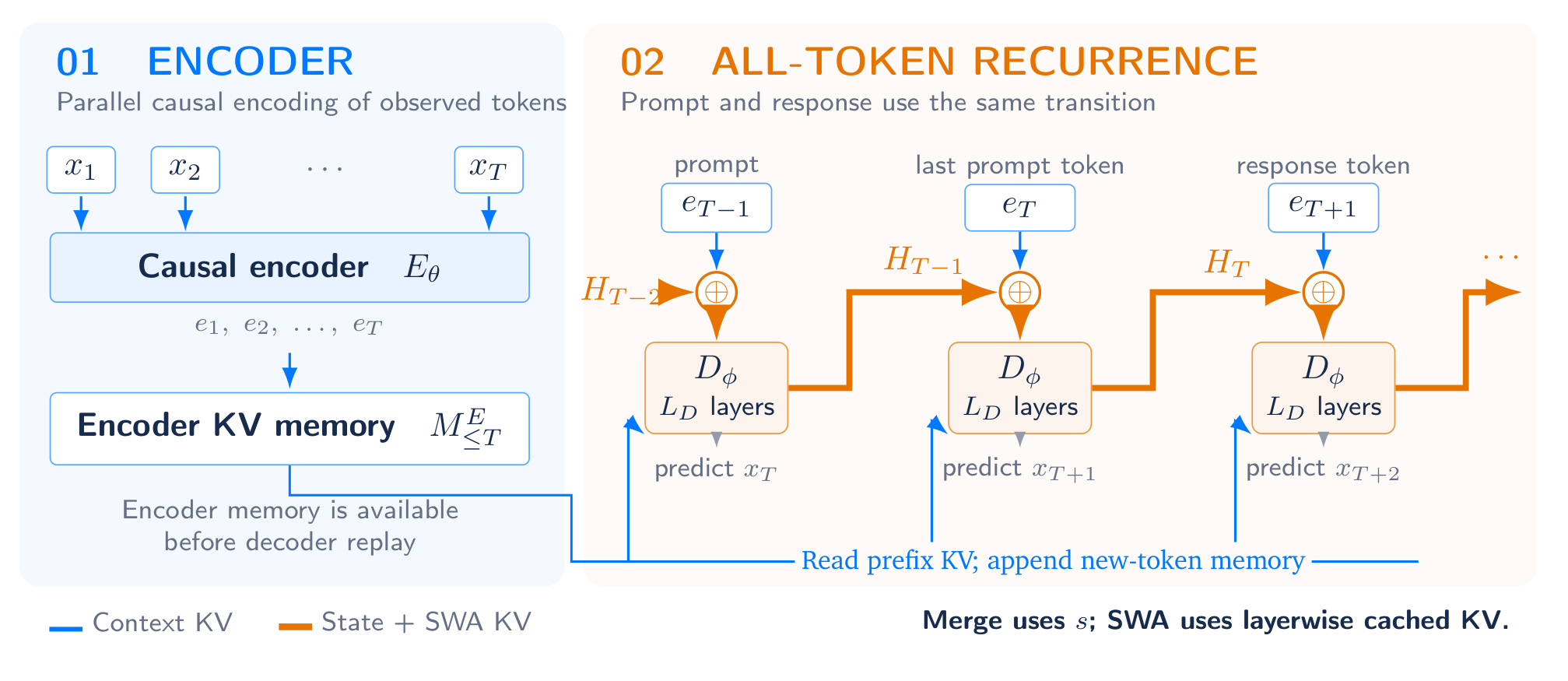
The progression begins with architectural foundations and formal state transitions before advancing to hardware execution dynamics, multi-phase training regimes, reinforcement learning replay semantics, and multi-turn serving. Central to RLT is the division of labor between a causal encoder and a recurrent decoder: the encoder constructs key-value context memory that can be computed in parallel across prefix tokens, while the recurrent decoder advances a persistent state and a bounded sliding-window attention cache across every token. A gated merge operation injects prior top-level decoder outputs directly into current encoder representations, creating a continuous recurrent loop across both prompt and response sequences without artificial state resets at serving boundaries. The text formalizes optional depth-wise parameter tying between compatible encoder and decoder layers, distinguishing parameter reuse from activation sharing.

Building upon this architectural core, the book details practical systems implementations and rigorous optimization protocols. Readers will learn how to design execution schedules that batch independent decoder updates, reuse resident key-value caches, and deploy activation checkpointing to preserve exact backpropagation through time across long contexts. The volume establishes exact mathematical and algorithmic requirements for autoregressive pretraining, supervised fine-tuning with masked assistant losses, and reinforcement learning policy optimization. For reinforcement learning, it details an exact replay contract: trainers reconstruct full-history hidden states under current network parameters while pairing them with sampler-recorded behavior probabilities, resolving policy mismatch across training and inference.

After studying this material, readers will be equipped to implement recurrent Transformer models, design cache-exact serving engines for multi-turn dialogues with external tool integrations, and structure replay pipelines for policy optimization. The book explicitly bounds its scope to the formal structural and mathematical definitions of RLT; it excludes empirical benchmark evaluations, measured hardware speedups, scaling curves, automated neural architecture searches, and alternative non-recurrent attention approximations.

1 Introduction

Section Summary: The Recurrent Looped Transformer aims to enable ongoing latent reasoning that grows deeper with each processed token, while also aligning the model design with both hardware constraints for efficient execution and reinforcement learning needs for consistent training and sampling. It achieves this through a causal encoder that builds shared context memory and a recurrent decoder whose state carries forward continuously across an entire sequence, allowing computation to extend indefinitely without resetting between prompts and generated outputs. This setup supports hardware-friendly optimizations such as batching and weight reuse, while ensuring the same history-based transitions apply uniformly during pretraining, fine-tuning, and reinforcement learning.

Recurrent Looped Transformer (RLT) is organized around three goals: latent reasoning with infinite depth, model–hardware co-design for efficient training and inference, and model–RL algorithm co-design for consistent training and sampling. We use infinite depth to mean that temporal computation has no fixed architectural bound as more tokens are processed. Every finite sequence still executes a finite computation.

A causal encoder constructs context memory, and a deep recurrent decoder merges each token's encoder representation with the previous decoder output. The state evolves over both observed prompts and generated responses, without restarting at their boundary. For a 48-layer encoder and 48-layer decoder, every token feeds $h_{t-1}^{96}$ into the computation beginning from $h_t^{48}$. Compatible weights can be shared between the two stacks, giving two logical passes through one backbone and 96 logical block evaluations per token.

Latent reasoning with infinite depth. The recurrent state transmits continuous intermediate computation directly between tokens. After $t$ processed tokens, a state path traverses $t L_D$ decoder blocks. Its depth is not capped by the number of stored layers: processing further tokens extends it. This supports a form of latent reasoning carried across the sequence, while keeping per-token block count fixed. The architecture makes that path available; learning useful reasoning along it is a separate question.

Model–hardware co-design. Encoder-derived memory decouples parallel feature construction from recurrent state updates. The resulting execution admits bulk encoder kernels, batching of independent decoder transitions across sequences, reuse of resident weights and KV, and checkpointed backward computation. These are the hardware optimization opportunities exposed by the architecture. Full prompt recurrence remains part of the model, so hardware efficiency must be pursued without silently skipping its sequential work.

Model–RL algorithm co-design. The same history-dependent transition defines pretraining, supervised fine-tuning, sampling, and RL replay. Current-policy states are reconstructed from the full history under current parameters, while behavior log-probabilities remain tied to the sampler that produced the actions. This resolves the structural mismatch caused by different prompt/response computations and establishes a consistent policy-evaluation basis for reliable RL scaling. Numerical discrepancies, ordinary policy lag, and the quality of the RL objective remain separate concerns.

Encoder-memory architectures such as YOCO motivate memory reuse (Sun et al., 2024), while Feedback Transformer, Recurrent Transformer, Full-bandwidth Transformer, $\text{T}^2\text{MLR}$, and Latent Recurrent Transformer establish important precedents for temporal feedback (Fan et al., 2020; Oncescu et al., 2026; Wang et al., 2026; Cai et al., 2026; Huang et al., 2026). Our focus is the full-decoder recurrence and the joint specification of its hardware execution and RL replay semantics. The report develops these mechanisms; it does not report measured efficiency or scaling results.

2 Method

Section Summary: The method models token sequences with a causal encoder that produces representations and a global key-value memory, paired with a decoder that maintains a recurrent state consisting of a hidden vector and a bounded sliding-window cache of prior decoder projections. For each token the encoder output is merged with the preceding decoder state via a learned gate; the decoder then applies sliding-window self-attention over its own cache, cross-attention to the encoder memory, and a feed-forward layer to produce an updated state and next-token distribution. The same transition is used for prompt prefill, which builds the complete state through successive updates, and for incremental generation, which continues from that state without resetting caches or altering the conditioning.

2.1 Sequence and state

Let $x_{1:S}$ be an independent sequence with $x_1 = \text{BOS}$. For inference, $x_{1:T}$ is the observed prompt and later tokens form a continuation. The index $T$ marks a serving boundary, not a change in the conditional model. Let $L_E, L_D$ be encoder and decoder depths and $d$ the residual width. We use column vectors. The encoder representation is $e_t \in \mathbb{R}^d$ and recurrent output is $s_t \in \mathbb{R}^d$. The complete decoder state is $H_t = (s_t, C_t^D)$, where $C_t^D$ contains the retained key/value projections at every decoder SWA layer. The window size $W \ge 1$ includes the current token. After each update, the cache retains at most $W - 1$ positions per layer for the next update. All parameters, including the learned initial state $s_\star$, are collected in $\Theta$; $E_\theta$ and $D_\phi$ denote its encoder and decoder components.

2.2 Causal encoder and memory

For an observed prefix, compute

$ e_{1:T} = E_\theta(x_{1:T}).\tag{2.1} $

Positions within each encoder layer can be processed together using a causal mask. Encoder layers remain sequential. For decoder memory group $g \in {1, \ldots, G}$, construct

$ k_t^g = P_K^g(e_t, t), \quad v_t^g = W_V^g \operatorname{RMSNorm}E(e_t), \quad M{\le t}^g = {(k_j^g, v_j^g)}_{j=1}^t.\tag{2.2} $

The key map includes normalization, projection, and any positional transformation. Decoder layer $\ell$ reads group $g(\ell)$; $G = 1$ shares memory across layers and $G = L_D$ permits layer-specific projections. This global memory depends on encoder representations, not decoder states. The reference decoder combines cross-attention to this memory with causal SWA over decoder activations. The two stores have distinct roles: $M_{\le t}$ supplies global encoder context, while $C_t^D$ supplies a bounded window of decoder-derived KV.

2.3 One transition for every token

Initialize once, before BOS:

$ H_0 = (s_\star, \emptyset).\tag{2.3} $

For every observed or sampled token, apply

$ u_t = \operatorname{Merge}(e_t, s_{t-1}),\tag{2.4} $

$ H_t = (s_t, C_t^D) = D_\phi(u_t; M_{\le t}, C_{t-1}^D, t), \quad t \ge 1,\tag{2.5} $

$ p_\Theta(x_{t+1} \mid x_{1:t}) = \operatorname{softmax}(W_o \operatorname{RMSNorm}o(s_t)){x_{t+1}}.\tag{2.6} $

Define $F_t(H) = D_\phi(\operatorname{Merge}(e_t, s); M_{\le t}, C^D, t)$ for $H = (s, C^D)$. For a fixed token sequence, encoder features have no direct dependency on decoder states. Nevertheless, the complete state used to predict the first response token includes every prompt transition:

$ H_T = F_T \circ F_{T-1} \circ \cdots \circ F_1(H_0).\tag{2.7} $

Generation continues from $H_T$. After sampling $x_{T+1}$ from $s_T$, encode it incrementally, append its encoder-derived KV, and compute $H_{T+1} = F_{T+1}(H_T)$, including every decoder SWA cache update. Neither component of $H_T$ is reset at the serving boundary.

2.4 Prompt prefill and incremental decoding

Prefill first computes the causal encoder representations and memory of the prompt, then evaluates $H_1, \ldots, H_T$ in order. At decoder position $t$, attention is restricted to $M_{\le t}$ even though the entire prompt memory is available. Generation uses

$ (e_t, C_t^E) = E_\theta^{\text{step}}(x_t, C_{t-1}^E)\tag{2.8} $

with encoder cache $C^E$, followed by memory append and the same decoder transition. Observed tokens can be encoded in chunks, provided the causal encoder cache is preserved and every token still receives its decoder update. Parallel encoder processing and recurrent encoder stepping are execution schedules for the same causal computation; there is no corresponding ordinary fully parallel schedule assumed for the nonlinear decoder recurrence. In particular, historical decoder KV must be produced by the preceding recurrent updates; a standard parallel SWA decoder pass is not generally equivalent.

2.5 Merge and decoder blocks

A concrete gated merge is

$ r_{t-1} = \operatorname{RMSNorm}s(s{t-1}),\tag{2.9} $

$ g_t = \sigma(W_g[e_t; r_{t-1}] + b_g),\tag{2.10} $

$ u_t = e_t + \alpha, g_t \odot W_s r_{t-1}.\tag{2.11} $

Here $W_g \in \mathbb{R}^{d \times 2d}$, $W_s \in \mathbb{R}^{d \times d}$, and $\alpha$ controls the feedback scale. A modest nonzero initial feedback scale is a candidate initialization, not an established stability prescription. Scalar gating or a low-rank $W_s$ reduces overhead.

For $z_t^0 = u_t$, a concrete decoder block first performs causal SWA, then encoder-memory cross-attention, then an FFN:

$ q_t^{D,\ell} = P_Q^{D,\ell}(z_t^{\ell-1}, t),\tag{2.12} $

$ k_t^{D,\ell} = P_K^{D,\ell}(z_t^{\ell-1}, t), \quad v_t^{D,\ell} = W_V^{D,\ell} \operatorname{RMSNorm}_{S,\ell}(z_t^{\ell-1}),\tag{2.13} $

$ b_t^\ell = z_t^{\ell-1} + \operatorname{Attn}\ell^D\left(q_t^{D,\ell}, {(k_j^{D,\ell}, v_j^{D,\ell})}{j=\max(1, t-W+1)}^t\right),\tag{2.14} $

$ a_t^\ell = b_t^\ell + \operatorname{Attn}\ell^M\left(P_Q^{M,\ell}(b_t^\ell, t), M{\le t}^{g(\ell)}\right),\tag{2.15} $

$ z_t^\ell = a_t^\ell + \operatorname{FFN}\ell(\operatorname{RMSNorm}{D,\ell}(a_t^\ell)), \quad s_t = z_t^{L_D}.\tag{2.16} $

The attention operators include their output projections; query/key maps include their respective normalizations and positional transformations. At each layer, current KV is formed before SWA, using the layer input, so current-position attention introduces no circular dependency. Historical decoder KV comes from $C_{t-1}^D$. After the update, retain positions $\max(1, t - W + 2), \ldots, t$ in $C_t^D$; this set is empty for $W = 1$. Position metadata follows the same convention during prefill, sampling, and replay. Alternative sublayer orders define different variants and must be used consistently in all execution modes.

2.6 What is looped: a concrete tied configuration

The reference tied RLT sets $L_E = L_D = L$. Encoder self-attention at layer $\ell$ and decoder SWA at layer $\ell$ share compatible query, key, value, and output projection matrices; their FFNs are also shared. The encoder uses its causal context, whereas decoder SWA uses decoder activations within its window. Decoder cross-attention has separate query/output projections and the memory projections of Equation (2.2). Stage-specific normalizations, the merge, and readout remain explicit modules. Thus a decoder block adds cross-attention to the reused attention/FFN core; two logical passes do not imply equal per-block FLOPs.

This is parameter reuse with different attention wiring, not activation copying. No decoder output is identified with an encoder output. An untied $E_\theta, D_\phi$ preserves the complete-state recurrence while removing depth-wise parameter reuse. Encoder-memory group sharing is an independent axis and does not merge or eliminate the layerwise decoder SWA caches.

3 Computational Properties

Section Summary: The section explains that the model produces identical internal states and output probabilities whether a prompt is processed all at once or token by token, because the underlying recurrence is mathematically invariant to where the prompt ends. It also details the computational costs of handling an initial prompt, noting that prefill work remains partly sequential through the decoder layers and that memory and cache requirements grow with context length. Finally, it shows that the recurrent path through decoder blocks can reach arbitrary depth over long sequences while keeping the per-token block count fixed, creating the potential for extended latent reasoning.

3.1 Prompt–response consistency

Proposition 3.1 (Invariance to the serving split). Fix the parameters, token sequence, position convention, and independent-sequence start state. Assume mathematically equivalent causal encoder execution, identical SWA windows and cache updates, and deterministic decoder operations. Processing any prefix by batched encoder prefill followed by recurrent decoder updates produces the same states and next-token distributions as processing that prefix incrementally. Moving the prompt–response split does not change the conditional distribution for a fixed token history.

Proof. Causal encoder equivalence gives the same $e_t$ and $M_{\le t}$ in both schedules. Both initialize with $H_0 = (s_\star, \emptyset)$. If their states agree at $t - 1$, Equation (2.5) applies identical operations to identical inputs at $t$, so their states agree at $t$. Induction establishes the result. The serving split never appears in the transition. $\square$

This is mathematical equivalence. Different kernels and precision choices can still cause numerical discrepancies. It also assumes identical tokenization and context, with no dropped tokens, reset, or stale state inserted in one execution.

3.2 Prefill work and sequential depth

Let $C_E^{\text{pf}}(T)$ be encoder prefill work, $C_M(T)$ the memory projection work, and $C_D^{\text{step}}(t)$ a decoder evaluation over $t$ encoder-memory entries and at most $W$ decoder positions per layer, including merge overhead. Then

$ C_{\text{prefill}}(T) = C_E^{\text{pf}}(T) + C_M(T) + \sum_{t=1}^T C_D^{\text{step}}(t).\tag{3.1} $

For dense attention and width-proportional KV, a coarse arithmetic estimate is

$ \mathcal{O}\left((L_E + L_D)(Td^2 + T^2d) + GTd^2 + L_D T \min(W, T)d\right).\tag{3.2} $

There is a sequential decoder path through $T$ transitions, each containing $L_D$ blocks. Encoder parallelism therefore does not imply fully parallel model prefill. State recurrence can reduce hardware utilization even when arithmetic order matches a conventional dense Transformer. We accept this cost to preserve full prompt computation; no reduced-prefill speedup is claimed.

Each new token evaluates $L_E + L_D$ blocks, plus merge and memory projection. Attention work still grows with context length. With effective KV width $d_{\text{KV}}$, inference cache storage is approximately

$ \mathcal{O}\left((L_E + G)t, d_{\text{KV}} + L_D \min(t, W - 1)d_{\text{KV}}^D + d\right).\tag{3.3} $

Here $d_{\text{KV}}^D$ is the effective decoder SWA KV width; the $\mathcal{O}(d)$ term is the current recurrent output. The SWA term counts retained history, excluding the transient current KV. Training activations are additional. Parameter tying reduces stored weights but does not eliminate the second logical pass or either cache role.

3.3 Latent reasoning with infinite temporal depth

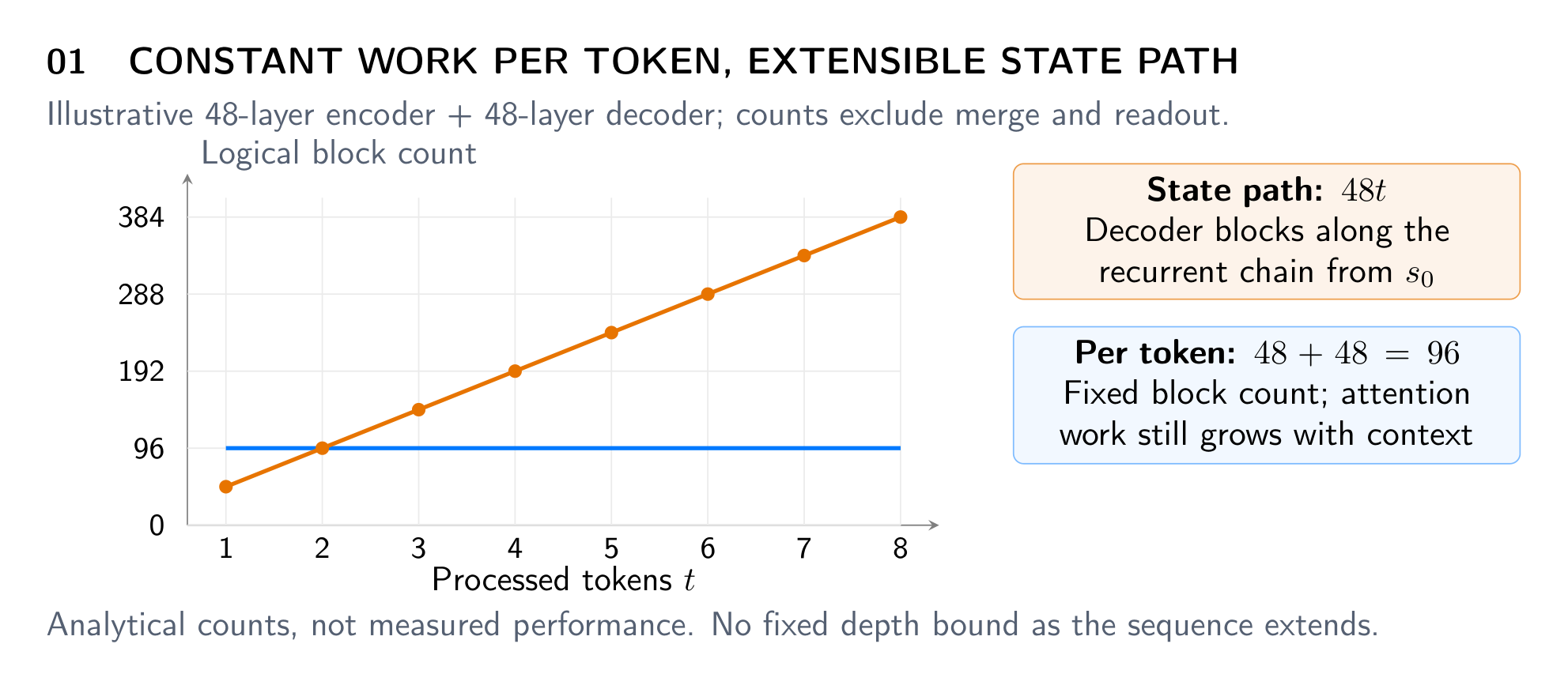
The available state path to position $t$ composes $t$ decoder transitions, traversing $t L_D$ decoder blocks from the sequence start. For a prompt of length $T$ followed by $n$ processed continuation tokens, the corresponding path contains $(T + n)L_D$ decoder blocks. Figure 2 illustrates these analytical counts. This depth includes the prompt and grows with the processed history while per-token block count stays fixed. Gates, contraction, and learned projections may suppress the practical contribution of long paths; structural depth alone is not a reasoning guarantee.

4 Model–Hardware Co-design

Section Summary: The section on model-hardware co-design explains how to run a recurrent neural network efficiently by computing fixed encoder features in parallel across tokens or sequences while batching decoder updates only when independent requests become ready, thereby exposing parallelism without violating the model's sequential state dependencies. It also covers memory strategies such as reusing immutable encoder key-value caches, maintaining separate short decoder windows, sharing memory groups, and fusing operations like normalization or gating to cut data movement and parameter storage. Finally, the text stresses that training relies on activation checkpointing and careful batching to fit within hardware limits, while insisting that all implementation choices preserve exact computational fidelity so the trained model behaves as intended on real devices.

4.1 Parallel work around a recurrent core

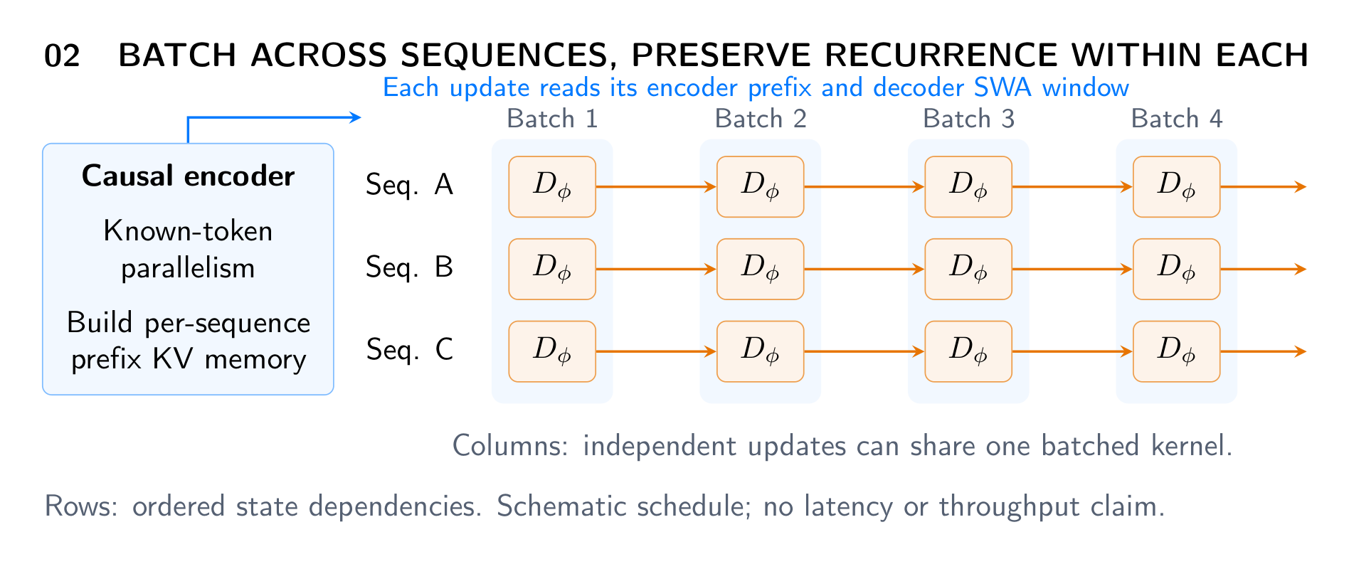
For a known training sequence or prompt, encoder features and memory projections can be computed with token-parallel kernels. Decoder evaluation then follows the state dependencies. As illustrated in Figure 3, across independent sequences, ready decoder transitions can be batched: each sequence contributes its next state update while maintaining its own encoder KV prefix, decoder SWA cache, recurrent output, and position. This exposes batch-level parallelism without asserting sequence-level parallelism within the recurrent decoder.

During inference, the encoder step, memory append, merge, decoder blocks, and readout form a repeated execution schedule. Scheduling independent requests together can increase matrix-operation sizes and weight reuse. Small batches or uneven sequence lengths may limit utilization. No exact parallel scan for the general nonlinear decoder is assumed.

4.2 Memory traffic and parameter reuse

Encoder-derived KV is immutable for a fixed token prefix and parameter set. Decoder layers read this memory and separately append decoder-derived KV to their bounded layerwise SWA caches. These caches cannot be replaced by encoder memory. Sharing memory groups reduces stored KV and projections, while choosing more groups preserves layer-specific memory transformations. Tying compatible encoder/decoder weights reduces the stored parameter footprint and can favor weight residency, but does not by itself reduce block evaluations or guarantee lower latency.

Normalization, gating, state projection, and residual addition are candidates for fused execution where dependencies and numerical semantics permit. Cross-attention should read only valid encoder-prefix memory, and SWA only its valid local window; a faster kernel that reads future entries changes the model. These are implementation targets, not claims of completed kernels or measured bandwidth savings.

4.3 Training memory and execution fidelity

Activation checkpointing trades recomputation for activation storage while retaining full BPTT. Encoder batching, decoder batching across examples, and checkpoint placement should be chosen jointly with sequence lengths and accelerator memory. The optimization target is useful training and inference throughput under the reference recurrent computation, rather than eliminating recurrence by approximation.

Zhang et al. (2026) frame the executed policy as a function of both weights and execution choices, including precision, cache construction, reductions, and sampling transforms. Hardware and algorithm choices meet at replay fidelity: kernel precision, stochastic operations, positional conventions, and cache lifetimes must be consistent with the policy being evaluated. Full prompt recurrence incurs a real cost. Co-design aims to execute that computation efficiently; hardware-efficient training and inference remain engineering goals until measured.

5 Training Objectives

Section Summary: The training objectives begin with autoregressive pretraining that teaches the model to predict each next token across full sequences, jointly updating the encoder, recurrent memory, and decoder. Supervised fine-tuning then restricts the loss to assistant-generated tokens while still allowing gradients to flow through all prior context without resetting internal state. For reinforcement learning, the setup requires exact on-policy or importance-weighted gradients computed via full backpropagation through time, with the trainer always replaying and differentiating the current recurrent computation rather than relying on stale cached states from sampling.

5.1 Autoregressive pretraining

Full-sequence next-token prediction is the base objective:

$ \mathcal{L}{\text{PT}}(\Theta) = -\mathbb{E}{x_{1:S}}\left[\frac{1}{S - 1}\sum_{t=1}^{S-1} \log p_\Theta(x_{t+1} \mid x_{1:t})\right].\tag{5.1} $

Initialize $H_0 = (s_\star, \emptyset)$, compute causal encoder features, and unroll the complete decoder state over positions $1, \ldots, S - 1$. Every non-BOS target is supervised. Encoder, memory projections, merge, and decoder train jointly. Independent documents reset recurrent outputs, decoder SWA caches, encoder caches, and positions, and use disjoint attention masks. Full documents or segments with a declared initial-context convention must be used; a segment cut cannot silently discard state while claiming full-history likelihood.

5.2 Supervised fine-tuning

Let $m_{t+1} = 1$ for assistant targets and 0 for user, system, tool, or padding targets. For examples with at least one selected target, optimize

$ \mathcal{L}{\text{SFT}}(\Theta) = -\mathbb{E}x\left[\frac{1}{\sum{t=1}^{S-1} m{t+1}}\sum_{\substack{1 \le t < S \ m_{t+1}=1}} \log p_\Theta(x_{t+1} \mid x_{1:t})\right].\tag{5.2} $

Loss masking does not mask state updates or detach encoder memory, recurrent outputs, or decoder KV. The decoder processes all preceding context tokens, including user and tool messages. Gradients from assistant losses can flow through those prompt computations. The state is not reset at an assistant boundary, and no separate boundary-adaptation objective is needed to repair a prompt-specific transition change.

5.3 Model–RL algorithm co-design

Let $c = x_{1:T}$ be a prompt and $y = (y_1, \ldots, y_N)$ a sampled response, with $y_i = x_{T+i}$. The policy is

$ \pi_\Theta(y \mid c) = \prod_{i=1}^N p_\Theta(y_i \mid c, y_{<i}).\tag{5.3} $

For a sequence reward $R(c, y)$ independent of $\Theta$, define $J(\Theta) = \mathbb{E}{c,, y \sim \pi\Theta}[R(c, y)]$. Its on-policy score-function gradient is

$ \nabla_\Theta J = \mathbb{E}{c,, y \sim \pi\Theta}\left[(R(c, y) - b(c))\sum_{i=1}^N \nabla_\Theta \log p_\Theta(y_i \mid c, y_{<i})\right],\tag{5.4} $

where $b(c)$ is a response-independent baseline, treated as constant in the policy gradient. Discrete sampled tokens are held fixed during log-probability replay, while differentiation includes their continuous recurrent computations. No particular reward function, clipping rule, or KL regularizer is required by the architecture.

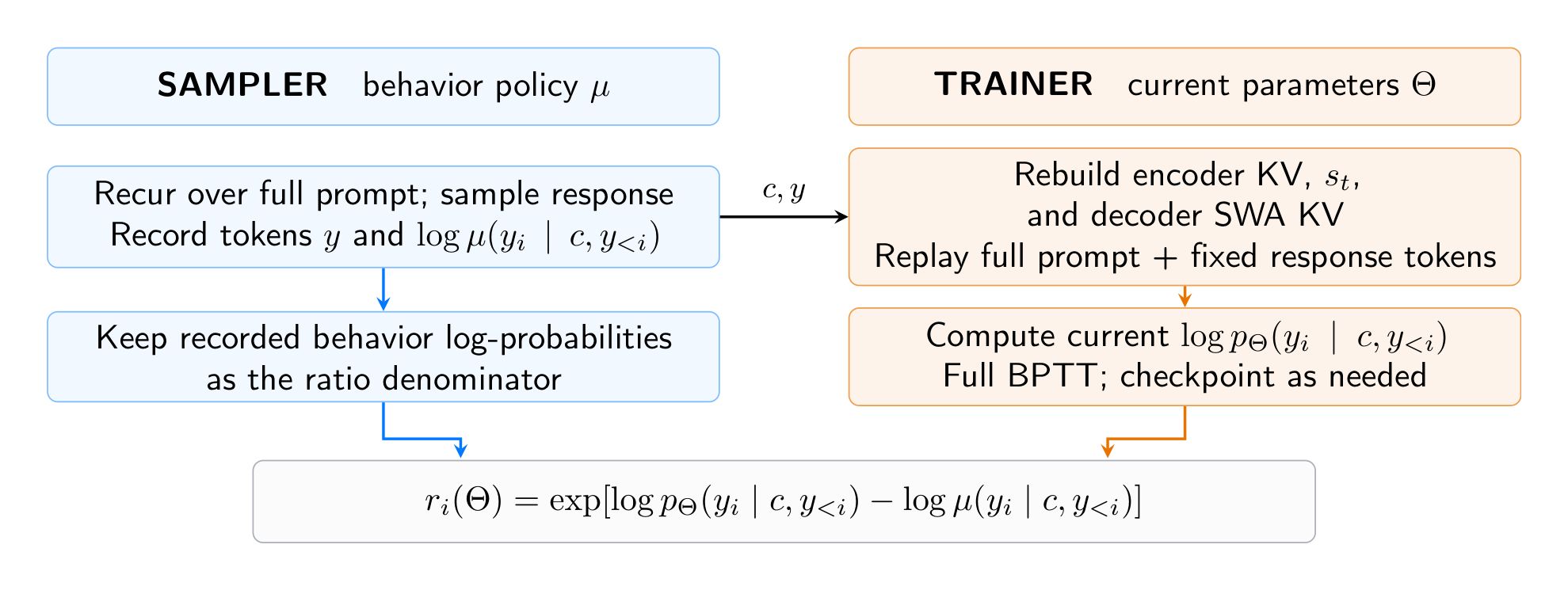
Figure 4 summarizes the replay contract. The sampler records each action's behavior log-probability under its actual sampling distribution $\mu$. For a trainer update at parameters $\Theta$, recompute causal encoder features with those parameters and reconstruct both the recurrent output and every decoder SWA cache over the full prompt and sampled response prefix, starting from the same sequence initialization. This yields current-policy log-probabilities and the token ratios

$ r_i(\Theta) = \exp\left(\log p_\Theta(y_i \mid c, y_{<i}) - \log \mu(y_i \mid c, y_{<i})\right).\tag{5.5} $

At identical parameters and sampling conventions, trainer and sampler represent the same computation. A raw model distribution must not be conflated with a temperature-scaled or truncated sampling distribution. Exact importance sampling requires $p_\Theta(\cdot \mid h) \ll \mu(\cdot \mid h)$ at relevant histories. Top-$k$ or top-$p$ behavior sampling generally violates this condition for an untruncated softmax target. Behavior log-probabilities must include temperature, truncation, and renormalization; metadata alone cannot restore missing support. Here the target is the raw model policy $p_\Theta$. A transformed target requires replacing the target probabilities consistently throughout the objective and ratios.

Following the execution-level distinction of Zhang et al. (2026), matching forward probabilities at one parameter value is not sufficient to establish matching policy gradients: the trainer must differentiate the recurrent target computation or a forward-and-backward equivalent implementation. RLT therefore specifies both full-history forward replay and its gradient path. A shared architectural transition alone does not prove numerical kernel parity.

Correct log-probabilities do not make an arbitrary off-policy loss unbiased. For fixed prompts and sequence rewards, exact trajectory importance sampling uses $\prod_i r_i$, subject to support and integrability. Tokenwise clipping or other surrogate objectives introduce their own algorithmic choices. Architecture-induced state mismatch and ordinary policy lag are distinct issues.

5.4 Gradients, checkpointing, and state staleness

Teacher forcing allows a parallel causal encoder pass over known tokens. Decoder replay remains sequential across the complete history. Full BPTT differentiates through encoder memory, recurrent outputs, and decoder SWA KV across prompt and response, even when losses are applied only to response tokens. Running prompt recurrence under no_grad preserves the forward probabilities if the state is recomputed at current parameters, but omits prompt-state derivatives and is a gradient approximation.

The reference training computation uses full BPTT with activation checkpointing as needed. Checkpointing recomputes forward operations during backward with the same parameters and stochastic state; it changes memory and compute costs without intentionally truncating gradients. Truncated BPTT is an optional approximation: preserve numeric values but detach explicitly selected boundary tensors. Detaching only $s_t$ leaves gradient paths through decoder KV and encoder memory; the truncation specification must identify all retained and detached paths. It can preserve current-policy forward probabilities while shortening the gradient horizon.

Within one replay, keep parameters fixed. After an optimizer update, previously computed encoder KV, recurrent outputs, and decoder SWA KV generally cease to be current-policy values. Recompute them from the sequence start, or from an exact prefix checkpoint produced under the same parameters and execution convention. This applies to every repeated optimization pass over a rollout. A sampler's old hidden states cannot replace current-policy replay. Conversely, its recorded behavior log-probabilities remain the denominators for the policy that actually sampled the actions.

6 Multi-turn Serving and Cache Semantics

Section Summary: In multi-turn conversations, new messages, tool results, and generated tokens are added to a running token history while reusing cached encoder and decoder states so generation can resume from the prior point without a full reset. A complete snapshot of those states, along with metadata and model version, can be saved and reloaded for continued inference as long as the underlying model weights remain unchanged, though edits, deletions, or rewrites to earlier content require recomputing from a valid earlier checkpoint rather than patching the existing cache. External tokens supplied during reinforcement learning still update the full state differentiably but are not counted as actions taken by the policy itself.

A conversation is serialized into a token history beginning at BOS. New user messages, tool results, role delimiters, and assistant tokens all receive encoder and decoder updates. At a tool return, encode the newly observed span using the cached encoder prefix, then advance the decoder through every new token from its existing state. Resume generation without resetting. The reference policy resets only at a new independent sequence or an explicitly defined context reset.

An exact prefix snapshot contains encoder cache $C_t^E$, encoder-derived cross-attention memory $M_{\le t}$, complete decoder state $H_t = (s_t, C_t^D)$, token and position metadata, the SWA window convention, and the model version. A compatible fixed-weight snapshot can be reused for inference because the state is independent of where the serving split was placed. Reproducing sampled outputs also requires the sampler's random state. Text-only restoration requires replay to rebuild hidden state; weight updates invalidate old-state reuse for exact current-policy computation.

Deleting, editing, or truncating a prefix changes the conditioning history. Recompute from a valid earlier checkpoint rather than retaining a state that includes removed content. Similarly, appending a template that rewrites earlier tokens is not an append-only cache operation. In multi-turn RL, externally supplied tokens update the complete state but are not sampled policy actions and do not receive action importance-ratio factors. Their state updates remain differentiable for full BPTT.

7 Related Work

Section Summary: The related work section surveys prior efforts to blend recurrent processing with transformer architectures for language modeling, including hybrids that pair transformer encoders with recurrent decoders, encoder-derived key-value memory for later reuse, and various forms of temporal or cross-token feedback that carry hidden states forward across steps. It also covers latent recurrent models, continuous hidden-state reasoning outside token space, block-level state propagation, and depth-wise computation reuse, noting how each approach manages parallelism, memory, and training stability. RLT is positioned as an extension of these ideas through its encoder-memory and recurrent-decoder split with final-output feedback, while differing in its use of full sequential replay over the entire history and token-level updates rather than block or auxiliary latent steps.

Hybrid Transformer–RNN models. Chen et al. (2018) combine a Transformer encoder with an RNMT+ decoder built from LSTMs, demonstrating an early hybrid of parallel attention-based encoding and recurrent generation for machine translation. RLT shares this broad division of labor. Its recurrent transition is instead a stack of Transformer blocks with encoder-memory cross-attention and decoder SWA, and it advances over every prompt and response token in one causal language model. Combining a Transformer encoder with recurrent decoding is therefore an established idea.

Encoder-derived memory. YOCO builds reusable KV memory for an upper cross-decoder and enables prefill early exit (Sun et al., 2024). DeepSeek-V4.1-Flash projects decoder global KV from final encoder states and separately handles decoder SWA (DeepSeek-AI, 2026). RLT retains encoder-derived memory but processes every prompt token through its recurrent decoder. It therefore does not inherit prompt-wide decoder skipping from those designs.

Temporal feedback. Feedback Transformer exposes processed past representations to future computation (Fan et al., 2020). Recurrent Transformer forms each layer's persistent KV from that layer's output, with an exact tiling schedule that improves memory movement (Oncescu et al., 2026). RLT instead feeds the previous final decoder output into the next decoder input; its global attention memory is encoder-derived, while local SWA KV is decoder-derived. Both prompt and response now carry recurrence. The distinction lies in the feedback location and memory representation, not a claim of fully parallel RLT prefill. The layerwise RT tiling result is not automatically a kernel for this full-decoder recurrence.

Cross-token latent feedback. Full-bandwidth Transformer (Wang et al., 2026) fuses the previous top-layer hidden state with the next token embedding through a gated linear unit, preserving the Transformer stack and KV cache. It directly precedes RLT's use of continuous output-to-input feedback across tokens. Its scheduled multi-pass training shifts hidden states from one pass into the next to retain token-parallel teacher forcing, with a prefix mixin to address prompt/generation differences. RLT injects feedback at the encoder–decoder interface and uses sequential decoder replay over the complete history as its reference training computation, with encoder-derived global memory and separate decoder SWA caches.

$\text{T}^2\text{MLR}$ (Cai et al., 2026) feeds a cached middle-layer representation from the previous token into an earlier layer at the current position. Its experiments show that localized middle-layer recurrence can outperform recurrence across the full network; a deeper recurrent block is therefore not automatically preferable. Its parallel training approximates temporal states with a fixed number of Jacobi iterations and separately controls backward depth. RLT specifies final-decoder-output feedback through the entire decoder, with full-history forward replay and full BPTT as the reference; optional TBPTT changes the gradient horizon. These choices distinguish computation and training semantics, without establishing an empirical advantage over either approach.

Latent recurrent language models. Latent Recurrent Transformer (LRT) (Huang et al., 2026) reuses the previous token's high-level source-layer state through KV projection and residual injection, retaining the standard decoder-only backbone and one forward per generated token. This is a close precedent for cross-token, cross-layer feedback. Its interleaved parallel training refines subsets of positions from a shared state buffer. For RL, it initializes that buffer with detached rollout states to reduce rollout/recomputation mismatch. RLT instead specifies an encoder-memory/recurrent-decoder split and reconstructs the complete history under current parameters for exact policy replay; cached behavior states are not substitutes for current-policy states after an update.

Continuous latent computation. Coconut (Hao et al., 2024) feeds the last hidden state back as the next input embedding during a dedicated latent reasoning phase, trained through a curriculum that replaces textual reasoning steps with continuous thoughts. PonderLM-2 (Zeng et al., 2025) extends hidden-state feedback to pretraining by inserting latent thoughts between ordinary tokens, and uses Jacobi iterations to approximate their recurrent dependencies in parallel. Both establish hidden-state feedback as a mechanism for computation outside token space. RLT merges its persistent decoder output with each current token's encoder representation without introducing auxiliary latent positions or a separate latent mode. Its temporal depth grows with ordinary prompt and response tokens; this differs from allocating additional latent steps before emitting a token.

Block- and segment-level recurrence. Block-Recurrent Transformers (Hutchins et al., 2022) use attention and gated updates over a persistent set of state vectors, processing blocks of tokens in parallel within each recurrent step. Recurrent Memory Transformer (Bulatov et al., 2022) carries learned memory-token representations between sequence segments, implementing memory through the Transformer's input and output sequence. These works establish recurrent state propagation with attention and expose useful trade-offs between state capacity and within-block parallelism. RLT instead updates its final decoder output and layerwise SWA caches at every token, while retaining separately constructed encoder-derived global memory. Its reference computation therefore pays for token-level sequential recurrence and does not inherit their block-level training schedule.

Depth-wise reuse. Universal Transformers share computation across depth (Dehghani et al., 2018), and recurrent-depth latent reasoning iterates a recurrent block to scale computation (Geiping et al., 2025). RLT's state advances across tokens, while its tied configuration additionally shares compatible encoder and decoder weights. Neither weight tying nor temporal recurrence alone establishes novelty or a quality improvement.

8 Conclusion

Section Summary: RLT integrates three core ideas: enabling deep hidden reasoning over time, jointly designing the model with both hardware and reinforcement learning algorithms, and maintaining a continuous internal state that processes every token in a prompt or response using a fixed number of steps. By separating the encoder from memory and sharing the same transition rules with exact replay during training, the approach reduces mismatches between the model and its learning process while unlocking opportunities for efficient parallel work and memory use. The design is clearly defined on paper, but its real gains in reasoning ability, speed, and scalability remain to be shown through testing.

RLT combines three design principles: latent reasoning with unbounded temporal depth, model–hardware co-design, and model–RL algorithm co-design. A continuous decoder state extends computation across every prompt and response token, with a fixed number of blocks per token. Encoder-memory separation exposes parallel work, memory reuse, and checkpointing opportunities around the recurrent core. A shared transition and exact current-policy replay eliminate structural prompt-boundary mismatch between trainer and sampler, providing a foundation for reliable RL scaling. The computational definitions are explicit; realized reasoning quality, hardware efficiency, and scaling behavior require future validation.

References

Section Summary: This section compiles a list of academic papers and technical reports focused on advanced transformer architectures that incorporate recurrence, memory mechanisms, and latent-space reasoning to improve efficiency and depth in language models. The references span foundational works from 2018 on universal and feedback-based transformers through more recent 2024–2026 studies on block-recurrent designs, KV cache compression, and continuous latent processing. Most entries are arXiv preprints or model repository reports, highlighting ongoing research into scaling test-time compute and decoder optimizations.

Aydar Bulatov, Yuri Kuratov, and Mikhail S. Burtsev. Recurrent memory transformer. arXiv preprint arXiv:2207.06881, 2022. URL https://arxiv.org/abs/2207.06881.

Ziyang Cai, Xingyu Zhu, Yihe Dong, Yinghui He, and Sanjeev Arora. $\text{T}^2\text{MLR}$: Transformer with temporal middle-layer recurrence. arXiv preprint arXiv:2607.15178, 2026. URL https://arxiv.org/abs/2607.15178.

Mia Xu Chen, Orhan Firat, Ankur Bapna, Melvin Johnson, Wolfgang Macherey, George Foster, Llion Jones, Niki Parmar, Mike Schuster, Zhifeng Chen, Yonghui Wu, and Macduff Hughes. The best of both worlds: Combining recent advances in neural machine translation. arXiv preprint arXiv:1804.09849, 2018. URL https://arxiv.org/abs/1804.09849.

DeepSeek-AI. DeepSeek-V4.1-Flash: Pushing the limits of KV cache compression. Technical report, DeepSeek-AI, 2026. URL https://huggingface.co/deepseek-ai/DeepSeek-V4.1-Flash/resolve/main/DeepSeek_V41_Tech_Report.pdf. Sections 2.2 and 3.2.2; publicly available from the official DeepSeek model repository.

Mostafa Dehghani, Stephan Gouws, Oriol Vinyals, Jakob Uszkoreit, and Łukasz Kaiser. Universal transformers. arXiv preprint arXiv:1807.03819, 2018. URL https://arxiv.org/abs/1807.03819.

Angela Fan, Thibaut Lavril, Edouard Grave, Armand Joulin, and Sainbayar Sukhbaatar. Addressing some limitations of transformers with feedback memory. arXiv preprint arXiv:2002.09402, 2020. URL https://arxiv.org/abs/2002.09402.

Jonas Geiping, Sean McLeish, Neel Jain, John Kirchenbauer, Siddharth Singh, Brian R. Bartoldson, Bhavya Kailkhura, Abhinav Bhatele, and Tom Goldstein. Scaling up test-time compute with latent reasoning: A recurrent depth approach. arXiv preprint arXiv:2502.05171, 2025. URL https://arxiv.org/abs/2502.05171.

Shibo Hao, Sainbayar Sukhbaatar, DiJia Su, Xian Li, Zhiting Hu, Jason Weston, and Yuandong Tian. Training large language models to reason in a continuous latent space. arXiv preprint arXiv:2412.06769, 2024. URL https://arxiv.org/abs/2412.06769.

Zeyi Huang, Xuehai He, Liliang Ren, Yiping Wang, Baolin Peng, Hao Cheng, Shuohang Wang, Pengcheng He, Jianfeng Gao, Yong Jae Lee, and Yelong Shen. Latent recurrent transformer: Architecture exploration, training strategies, and scaling behavior. arXiv preprint arXiv:2605.26797, 2026. URL https://arxiv.org/abs/2605.26797.

DeLesley Hutchins, Imanol Schlag, Yuhuai Wu, Ethan Dyer, and Behnam Neyshabur. Block-recurrent transformers. arXiv preprint arXiv:2203.07852, 2022. URL https://arxiv.org/abs/2203.07852.

Costin-Andrei Oncescu, Depen Morwani, Samy Jelassi, Alexandru Meterez, Mujin Kwun, and Sham Kakade. The recurrent transformer: Greater effective depth and efficient decoding. arXiv preprint arXiv:2604.21215, 2026. URL https://arxiv.org/abs/2604.21215.

Yutao Sun, Li Dong, Yi Zhu, Shaohan Huang, Wenhui Wang, Shuming Ma, Quanlu Zhang, Jianyong Wang, and Furu Wei. You only cache once: Decoder-decoder architectures for language models. arXiv preprint arXiv:2405.05254, 2024. URL https://arxiv.org/abs/2405.05254.

Xi Wang, Ziyang Cai, Zheng Zhan, Harry Dong, Ying Fan, Gustavo de Rosa, Tim Pearce, and John Langford. Full-bandwidth transformer. arXiv preprint arXiv:2608.08888, 2026. URL https://arxiv.org/abs/2608.08888.

Boyi Zeng, He Li, Shixiang Song, Yixuan Wang, Ziwei He, Xinbing Wang, and Zhouhan Lin. PonderLM-2: Pretraining LLM with latent thoughts in continuous space. arXiv preprint arXiv:2509.23184, 2025. URL https://arxiv.org/abs/2509.23184.

Yifan Zhang et al. Reliable RL scaling requires accounting for Prefill–Decode kernel mismatch. Technical report, Pretraining-RL-Science project, August 2026. URL https://github.com/yifanzhang-pro/Pretraining-RL-Science/blob/master/Prefill_Decode_Kernel_Mismatch.pdf. Dated August 6, 2026; revised August 24, 2026.

Appendix

A Reference Execution Schedules

Section Summary: This section outlines standard procedures for initializing and updating a combined encoder-decoder model's internal state across different phases of operation. It covers recurrent processing of an initial prompt to build encoder memory and decoder caches, followed by sequential token generation or incorporation of external inputs while preserving exact update order. The same disciplined recurrence is then applied to full-sequence pretraining or supervised fine-tuning, as well as to replaying reinforcement-learning rollouts for policy-gradient computation.

The complete decoder state is $H_t = (s_t, C_t^D)$, with $H_0 = (s_\star, \emptyset)$. Encoder continuation state and encoder-derived cross-attention memory are maintained separately. All schedules use the block order and window convention in Equation (2.16).

A.1 Recurrent prompt prefill

1. Start an independent sequence with $x_1 = \text{BOS}$ and $H_0 = (s_\star, \emptyset)$; initialize encoder caches and positions.
2. Encode $x_{1:T}$ causally in parallel and construct its encoder KV memory.
3. For $t = 1, \ldots, T$, compute $H_t = D_\phi(\operatorname{Merge}(e_t, s_{t-1}); M_{\le t}, C_{t-1}^D, t)$. Each decoder layer reads only its permitted historical SWA entries and current KV. Never expose future encoder or decoder KV to an earlier query.
4. Predict the first response token from $s_T$. Preserve $H_T$, encoder caches, memory, and positional metadata for the next update.

Historical decoder KV is produced by the preceding recurrent updates. Parallel causal encoder prefill does not make an ordinary parallel SWA decoder pass equivalent to this recurrence.

A.2 Generation and new external inputs

Sample $x_{t+1}$ from the distribution predicted by $s_t$, then consume it by updating the encoder cache and memory and advancing the complete decoder state to $H_{t+1}$. The resulting state predicts $x_{t+2}$. Every consumed token receives exactly one recurrent update and one KV insertion at every decoder SWA layer.

When a user or tool supplies multiple tokens, their encoder representations can be computed in a causal batch conditioned on the existing prefix. Decoder updates still occur in token order from the saved complete state. External tokens update both $s_t$ and $C_t^D$.

A length-limited generation may defer consuming its final emitted token. The cache API must then record that pending token separately and consume it before any later token. The caches represent the consumed prefix, excluding the pending token. This prevents double or skipped updates on resume.

A.3 Pretraining and SFT

1. Compute $e_{1:S-1}$ using a causal encoder and construct memory.
2. Initialize $H_0 = (s_\star, \emptyset)$; unroll all positions $1, \ldots, S - 1$, including every layerwise SWA cache update.
3. Accumulate all valid next-token losses for pretraining, or only assistant-target losses for SFT. All context tokens receive state updates.
4. Normalize each example by its number of selected targets, then average examples as in Equations (5.1) and (5.2). Backpropagate through the complete computation, using checkpointing if required.

Examples without selected targets are excluded from the loss average. An alternative token-weighted batch normalization defines a different weighting of examples and should be stated explicitly.

Packed independent sequences use separate recurrent states, decoder SWA caches, encoder caches, positions, and attention masks. Neither attention mechanism may cross a document boundary. A loss mask never substitutes for an attention mask or a complete document-state reset. Training cache operations must preserve autograd dependencies or support equivalent recomputation.

A.4 Current-policy RL replay

1. Read the rollout token history, action mask, actual behavior log-probabilities, and sampling metadata. Behavior probabilities include all sampling transforms and renormalization.
2. Hold current parameter values fixed throughout forward replay and backward. Use the target policy's positional, SWA, and execution conventions without disabling parameter gradients.
3. Recompute encoder representations of the known history. From $H_0 = (s_\star, \emptyset)$, rebuild the recurrent output and every decoder SWA cache through all prompt tokens.
4. Replay subsequent tokens in order. Before consuming each sampled action, read its current-policy log-probability from the preceding state. Include EOS if sampled. Consume every intervening external token needed for later predictions.
5. Form the chosen RL loss from action log-probabilities, rewards or advantages, and any required behavior ratios. Do not assign policy-action factors to external user/tool tokens.
6. Backpropagate, update parameters, and invalidate parameter-dependent encoder and decoder caches before the next exact current-policy replay.

The action mask selects policy-loss terms only; it must not disable gradient tracking through external-token updates. All assistant turns are replayed with their intervening external context. Prompt replay under no_grad, or detaching prompt KV, can preserve forward values but is not the reference full-BPTT calculation.

Exact importance-sampling claims require support coverage at relevant histories. Recording the probability of a sampled action does not repair missing support for unsampled actions. The use of tokenwise or trajectory-level weighting is an RL-algorithm choice, not a consequence of the replay schedule.

A deterministic policy forward, such as one with dropout disabled, avoids ambiguity from internal stochastic computation. Otherwise the policy must specify how such randomness is conditioned on or marginalized; a single arbitrary stochastic replay is not generally the marginal action probability. Matching schedules alone does not establish numerical equality across kernels or precision settings.

B Causality and Gradient Paths

Section Summary: The section establishes that a causally masked encoder and decoder with sliding-window attention ensure the model's internal state at step t is shaped only by tokens up to t, with no leakage from future inputs. It then defines the Jacobian matrices that capture how gradients propagate backward through both the recurrent state and the decoder's cached key-value projections, showing that these paths are richer than those involving the state alone and are not automatically bounded by normalization. The discussion concludes by applying the chain rule to the full loss gradient with respect to parameters, noting that detaching boundary tensors such as the final state or encoder memory selectively removes certain gradient routes even though the forward computation remains unchanged.

Proposition B.1 (Causality). With a causal encoder, prefix-restricted encoder memory, and causal decoder SWA, $H_t = (s_t, C_t^D)$ depends only on $x_{1:t}$ and the parameters, including $s_\star$, under deterministic execution.

Proof. Encoder causality implies that each $e_j$ depends only on $x_{1:j}$, hence $M_{\le t}$ depends only on $x_{1:t}$. The initial state contains no future-token information. Suppose $H_{t-1}$ depends only on $x_{1:t-1}$. The next update uses this state, $e_t$, and $M_{\le t}$. At each decoder layer, current KV is formed from the causally available layer input, and SWA reads no position greater than $t$. Appending current KV and evicting old entries introduce no future information. Thus both $s_t$ and $C_t^D$ depend only on $x_{1:t}$, completing the induction. $\square$

For teacher-forced encoder features held fixed, use a fixed-slot representation of the decoder cache, with validity masks during warm-up, and define

$ J_t = \frac{\partial H_t}{\partial H_{t-1}}.\tag{B.1} $

Then

$ \frac{\partial H_t}{\partial H_j} = J_t J_{t-1} \cdots J_{j+1}, \quad j < t,\tag{B.2} $

where

$ J_t = \begin{pmatrix} \frac{\partial s_t}{\partial s_{t-1}} & \frac{\partial s_t}{\partial C_{t-1}^D} \ \frac{\partial C_t^D}{\partial s_{t-1}} & \frac{\partial C_t^D}{\partial C_{t-1}^D} \end{pmatrix}.\tag{B.3} $

A product involving only $\partial s_t / \partial s_{t-1}$ generally misses paths through decoder KV. Normalization alone does not bound products of these Jacobians.

Encoder memory provides access to past encoder information. Decoder SWA additionally exposes cached projections of recent decoder activations. Neither is an unrestricted archive of all previous decoder states. Evicted entries can still influence later computation through states or retained activations that previously consumed them.

Full parameter derivatives also include the parameter dependence of encoder features, memory, every transition, and decoder KV projections. Let $B_T^E$ denote all encoder-side boundary tensors needed for response continuation, including encoder continuation KV and encoder-derived cross-attention memory. For a response loss $\ell(\Theta, H_T(\Theta), B_T^E(\Theta))$, the chain rule gives

$ \frac{\mathrm{d}\ell}{\mathrm{d}\Theta} = \frac{\partial \ell}{\partial \Theta} + \frac{\partial \ell}{\partial H_T} \frac{\partial H_T}{\partial \Theta} + \frac{\partial \ell}{\partial B_T^E} \frac{\partial B_T^E}{\partial \Theta}.\tag{B.4} $

The first term holds the boundary arguments fixed; the other terms account for their prefix computation. In particular,

$ \frac{\partial \ell}{\partial H_T} \frac{\partial H_T}{\partial \Theta} = \frac{\partial \ell}{\partial s_T} \frac{\partial s_T}{\partial \Theta} + \frac{\partial \ell}{\partial C_T^D} \frac{\partial C_T^D}{\partial \Theta}.\tag{B.5} $

Detaching $s_T$, decoder KV, or encoder-side boundary tensors removes corresponding gradient paths even if forward probabilities are unchanged. None of these operations is full BPTT.

C Exactness of Cached States

Section Summary: A cached prefix can stand in for full recomputation only when every detail—model parameters, token sequence, positions, initialization, window rules, and policy settings—matches exactly, covering all recurrent states, decoder caches, and encoder memory. Detached or stale caches built under different weights cannot supply the gradient paths needed for training, so the original computation graph must be kept or redone. Methods such as truncated back-propagation or sliding-window eviction each cut specific dependencies in their own way, and these choices must be stated clearly because they are not interchangeable with simple cache reuse.

A cached prefix can replace forward replay for probability evaluation only when the complete cache matches the current parameters, consumed token prefix, positions, initialization, window semantics, and policy execution settings. It includes recurrent output, every decoder SWA cache, encoder continuation state, encoder-derived memory, and required metadata. Stochastic computation must be treated according to the policy definition.

A detached cache does not supply the derivative graph required for full-gradient training. The prefix graph must be retained or recomputed so gradients reach all parameter-dependent boundary tensors. A cache built under older weights generally satisfies neither the current-policy value nor the full-gradient requirement.

Activation checkpointing within one update recomputes activations under the same parameters and stochastic state. Mutable cache implementations must restore checkpointed contents during recomputation and must not overwrite activations still required by backward.

Truncated BPTT instead preserves numeric values while cutting selected gradient dependencies. A complete decoder-state detach is

$ \tilde{H}_t = (\operatorname{stopgrad}(s_t), \operatorname{stopgrad}(C_t^D)).\tag{C.1} $

Detaching only $s_t$ leaves possible paths through decoder KV; detaching only decoder KV leaves paths through the recurrent output. Encoder-side boundary tensors can provide additional paths across the same boundary. Any truncation scheme must state which tensors are detached.

SWA eviction limits future direct access to old KV; it is not itself a stop-gradient operation. Full BPTT still differentiates computations that consumed those entries before eviction. The inference cache size therefore does not bound full-BPTT activation storage.

Processing later chunks after changing weights while retaining earlier states or KV is a separate stale-state approximation. These distinctions apply equally to pretraining, SFT, and RL.