Towards Understanding Knowledge Distillation

Mary Phuong $^{1}$
IST Austria (Institute of Science and Technology Austria)

Christoph H. Lampert $^{1}$
IST Austria (Institute of Science and Technology Austria)

Abstract

Knowledge distillation, i.e. one classifier being trained on the outputs of another classifier, is an empirically very successful technique for knowledge transfer between classifiers. It has even been observed that classifiers learn much faster and more reliably if trained with the outputs of another classifier as soft labels, instead of from ground truth data. So far, however, there is no satisfactory theoretical explanation of this phenomenon. In this work, we provide the first insights into the working mechanisms of distillation by studying the special case of linear and deep linear classifiers. Specifically, we prove a generalization bound that establishes fast convergence of the expected risk of a distillation-trained linear classifier. From the bound and its proof we extract three key factors that determine the success of distillation: data geometry – geometric properties of the data distribution, in particular class separation, has an immediate influence on the convergence speed of the risk; optimization bias – gradient descent optimization finds a very favorable minimum of the distillation objective; and strong monotonicity – the expected risk of the student classifier always decreases when the size of the training set grows.

$^{1}$ IST Austria (Institute of Science and Technology Austria). Correspondence to: Mary Phuong [email protected].

Executive Summary: Knowledge distillation trains one classifier (the student) on the real-valued outputs of another (the teacher) rather than on ground-truth labels. Practitioners have repeatedly observed that this produces faster, more stable optimization and often better generalization, even when the teacher was itself trained on the same data. Yet until now there has been no quantitative theory explaining why the method works or when it works best.

This paper supplies the first such theory by restricting attention to binary classification with linear and deep-linear students. In this analytically tractable setting the authors derive an exact characterization of the weights learned by gradient flow on the distillation objective, prove a non-vacuous bound on the student’s expected disagreement with the teacher, and identify the mechanisms that drive success.

The analysis yields three concrete results. First, when the transfer set contains at least as many examples as the input dimension, the student recovers the teacher’s weight vector exactly and therefore achieves zero transfer risk. Second, with fewer examples the student recovers the projection of the teacher onto the span of the data; the resulting risk is bounded by a simple expression that depends on the angular alignment between the data distribution and the teacher. For distributions that possess an angular margin the bound decays exponentially in the number of examples; for polynomial-tailed alignments it decays essentially as ((\log n/n)^\kappa). Third, three factors explain these favorable rates: favorable data geometry (large angular separation speeds convergence), an optimization bias of gradient descent (it consistently reaches the most useful among many equally good minima), and strong monotonicity (adding any new transfer example can never increase the student’s angle to the teacher).

These properties are absent or far weaker in ordinary hard-label training, which explains why distillation often succeeds with small, finite data sets and little regularization. The same factors suggest practical leverage points: curating transfer sets whose geometry is well aligned with the teacher, initializing near the origin to preserve the favorable bias, and exploiting monotonicity when selecting which points to label.

The main limitation is that all results are proved only for linear and deep-linear models. Whether analogous mechanisms govern nonlinear networks remains an open question; the authors flag this extension as the principal direction for future work. Within the linear regime, however, the bounds and characterizations are tight and the supporting experiments on synthetic tasks and MNIST are consistent. Decision-makers can therefore treat the three identified factors as reliable design principles while awaiting nonlinear theory.

1. Introduction

Section Summary: In 2014 researchers noticed that training a new classifier by copying the real-valued outputs of an existing model, a technique called knowledge distillation, often worked better and more smoothly than training directly on the true labels, even when both models saw the same data. Practical successes have since been reported across many settings, yet almost no quantitative theory explains why the method succeeds. This paper therefore studies the simplest possible case—binary classification with linear models—and proves that distillation can drive the student’s error to zero from a finite training set while identifying three factors, data geometry, optimization bias, and strong monotonicity, that govern its rapid convergence.

In 2014, [1] made a surprising observation: they found it easier to train classifier using the real-valued outputs of another classifier as target values than using actual ground-truth labels. Calling the procedure knowledge distillation, or distillation for short, they noticed the positive effect to occur even when the existing classifier (called teacher) was trained on the same data as it used afterwards for the distillation-training of the new classifier (called students). Since that time, the positive properties of distillation-based training has been confirmed several times: the optimization step is generally more well-behaved than the optimization step in label-based training, and it needs less if any regularization or specific optimization tricks. Consequently, in several fields, distillation has become a standard technique for transfering the information between classifiers with different architectures, such as from deep to shallow neural networks or from ensembles of classifiers to individual ones.

While the practical benefits of distillation are beyond doubt, its theoretical justification remains almost completely unclear. Existing explanations rarely go beyond qualitative statements, e.g. claiming that learning from soft labels should be easier than learning from hard labels, or that in a multi-class setting the teacher's output provides information about how similar different classes are to each other.

In this work, we follow a different approach. Instead of studying distillation in full generality, we restrict our attention to a simplified, analytically tractable, setting: binary classification with linear teacher and linear student (either shallow or deep linear networks). For this situation, we achieve the first quantitative results about the effectiveness of distillation-based training. Specifically, our main results are: 1) We prove a generalization bound that establishes extremely fast convergence of the risk of distillation-trained classifiers. In fact, it can reach zero risk from finite training sets. 2) We identify three key factors that explain the success of distillation: data geometry – geometric properties of the data distribution, in particular class separation, directly influence the convergence speed of the student's risk; optimization bias – even though the distillation objective can have many optima, gradient descent optimization is guaranteed to find a particularly favorable one; and strong monotonicity – increasing the training set always decreases the risk of the student classifier.

2. Related Work

Section Summary: The concept of distillation, which involves transferring knowledge from one model to another, originated in early theoretical work and became popular after its use for compressing neural networks. Researchers have since applied it successfully to many tasks such as handling noisy data, improving robustness, and supporting distributed or privacy-preserving training, yet few studies have explained why it works from a mathematical standpoint; existing analyses frame it either as learning with privileged information or as a semi-supervised process that leverages extra unlabeled examples. The section also notes a connection to machine teaching, where carefully chosen examples allow efficient learning, though distillation achieves comparable benefits using more practical model-generated supervision, at least in linear cases.

Ideas underpinning distillation have a long history dating back to the work of [2, 3, 4, 5, 6]. In its current and most widely known form, it was introduced by [1] in the context of neural network compression.

Since then, distillation has quickly gained popularity among practitioners and established its place in deep learning folklore. It has been found to work well across a wide range of applications, including e.g. transferring from one architecture to another [7], compression [8, 9], integration with first-order logic [10] or other prior knowledge [11], learning from noisy labels [12], defending against adversarial attacks [13], training stabilization [14, 15], distributed learning [9], reinforcement learning [16] and data privacy [17].

In contrast to the empirical success, the mathematical principles underlying distillation's effectiveness have largely remained a mystery. Only very works examine distillation from a theoretical perspective. [18] cast distillation as a form of learning using privileged information (LUPI, [19]), a learning setting in which additional per-instance information is available at training time but not at test time. However, the LUPI view concentrates on the aspect that the teacher's supervision to the student is noise-free. This argument fails to explain, e.g., the success of distillation even when the original problem is noise-free to start with. The only other theoretical analysis we are aware of is by [20], who study distillation as a form of semi-supervised learning. Specifically, they show that a two-step procedure, consisting of first training a teacher on a small labelled dataset and then training the student on a separate large dataset labelled by the teacher, can be more effective than training the student directly on the small labelled dataset. The paper's focus is on the semi-supervised aspect, i.e. the gains from having a large unlabelled dataset.

A more distantly related topic is machine teaching [21]. In machine teaching, a machine learning system is trained by a human teacher, whose goal is to hand-pick as small a training set as possible, while ensuring that the machine learns a desired hypothesis. Transferring knowledge via machine teaching techniques is extremely effective: perfect transfer is often possible from a small finite teaching set [22, 23]. However, the price for this radical reduction in sample complexity is the expensive training set construction. Our work shows that, at least in the linear setting, distillation achieves a similar effectiveness with a more practical form of supervision.

3. Background: Linear Distillation

Section Summary: In binary classification, a fixed linear teacher model provides soft probabilistic labels via the sigmoid function on randomly sampled inputs, which are then used to train a student linear classifier (possibly parameterized as a deep linear network) by minimizing cross-entropy loss. Although the deep parameterization does not increase the student's expressive power, it alters the dynamics of gradient-based training, which is modeled here via continuous gradient flow. The section ultimately aims to bound the student's transfer risk, or probability of disagreeing with the teacher, as a function of the number of distillation samples.

We formally introduce distillation in the context of binary classification. Let $\mathcal X\subseteq \mathbb R^d$ be the input space, $\mathcal Y={0, 1}$ the label space, and $P_{\mathbf x}$ the probability distribution of inputs. We assume $P_\mathbf x$ has a density.

The teacher $h^*: \mathcal X\to \mathcal Y$ is a fixed linear classifier, i.e. $h^*(\mathbf x) = \mathbf{1}{\left{ \mathbf w_* ^\intercal \mathbf x \geq 0 \right}}$ for some $\mathbf w_*\in \mathbb R^d\setminus{\left{ \mathbf{0} \right}}$, where $\mathbf{1}{\left{ . \right}}$ returns 1 if the argument is true and 0 otherwise. The student also is a linear classifier, $h(\mathbf x) = \mathbf{1}{\left{ \mathbf w ^\intercal \mathbf x \geq 0 \right}}$.

We allow the weight vector to be parameterised as a product of matrices, $\mathbf w ^\intercal= \mathbf W_N \mathbf W_{N-1}\cdot s \mathbf W_1$ for some $N\geq 1$. When $N\geq 2$, this parameterisation is known as a deep linear network. Although deep linear networks have no additional capacity compared to directly parameterised linear classifiers $(N=1; \mathbf w ^\intercal= \mathbf W_1)$, they induce different gradient-descent dynamics, and are often studied as a first step towards understanding deep nonlinear networks [24, 25, 26].

Distillation proceeds as follows. First, we collect a transfer set ${\left{ (\mathbf x_i, y_i) \right}}{i=1}^n$ consisting of inputs $\mathbf x_i$ sampled i.i.d. from $P\mathbf x$, and soft labels $y_i=\sigma(\mathbf w_* ^\intercal \mathbf x_i)$ provided by the teacher, where $\sigma$ is the sigmoid function, $\sigma(x) = 1/(1+\exp(-x))$. The soft (real-valued) labels can be thought of as a more informative version of the hard (0/1-valued) labels of the standard classification setting. We write $\mathbf X={\left[\mathbf x_1, \dots, \mathbf x_n \right]}\in \mathbb R^{d\times n}$ for the data matrix. Second, the student is trained by minimizing the (normalized) cross-entropy loss,

$ \begin{split} L^1(\mathbf w) = -\frac 1 n \sum_{i=1}^n \Big[y_i\log \sigma(\mathbf w ^\intercal \mathbf x_i) \ + (1-y_i)\log(1-\sigma(\mathbf w ^\intercal \mathbf x_i))\Big] - L^*, \end{split}\tag{1} $

where $L^*$ is a normalization constant, such that the minimum of $L^1$ is 0. It only serves the purpose of simplifying notation and has no effect on the optimization.

The student observes the loss as a function of its parameters, i.e. the individual weight matrices,

$ L(\mathbf W_1, \dots, \mathbf W_N) := L^1((\mathbf W_N \mathbf W_{N-1}\cdot s \mathbf W_1)^\intercal),\tag{2} $

and optimizes it via gradient descent. For the theoretical analysis, we avoid the complications of stepsize selection and adopt the notion of infinitesimal step size[^1], which turns the gradient descent procedure into a continuous gradient flow. We write $\mathbf W_i(\tau)$ for the value of the matrix $\mathbf W_i$ at time $\tau\in [0, \infty)$, with $\mathbf W_i(0)$ denoting the initial value, and $\mathbf w(\tau)^\intercal = \mathbf W_N(\tau)\cdot s \mathbf W_1(\tau)$. Then, each $\mathbf W_i(\tau)$, for $i\in{\left{ 1, \dots, N \right}}$, evolves according to the following differential equation.

[^1]: For readers who are unfamiliar with gradient flows, it suffices to think of the stepsize as finite and "sufficiently small".

$ {\frac{\partial \mathbf W_i(\tau)}{\partial \tau}} = -{\frac{\partial L}{\partial \mathbf W_i}}(\mathbf W_1(\tau), \dots, \mathbf W_N(\tau)).\tag{3} $

The student is trained until convergence, i.e. $\tau\to\infty$. We measure the transfer risk of the trained student, defined as the probability that its prediction differs from that of the teacher,

$ R(h) = \operatorname{\mathbb P}{\mathbf x\sim P\mathbf x}{\left[h(\mathbf x) \neq h^*(\mathbf x) \right]}.\tag{4} $

In Section 4.2, we will derive a bound for the transfer risk and establish how rapidly it decreases as a function of $n$.

4. Generalization Properties of Linear Distillation

Section Summary: In the linear setting, distillation training enables a student model to exactly recover the teacher's underlying weight vector as soon as the number of examples reaches the data dimension, or otherwise to recover the closest approximation possible within the subspace spanned by those examples. This yields unusually strong generalization, with the student's risk falling to zero once enough data is present and otherwise admitting an explicit, distribution-dependent bound. The results also clarify the conditions under which distillation succeeds as a knowledge-transfer method.

This section contains our main technical results. First, in Section 4.1, we provide an explicit characterization of the outcome of distillation-based training in the linear setting. In other words, we identify what the student actually learns. In particular, we prove that the student is able to perfectly identify the teacher's weight vector, if the number of training examples ($n$) is equal to the dimensionality of the data ($d$) or higher. If less data is available, under minor assumptions, the student finds the best approximation of the teacher's weight vector that is possible within the subspace spanned by the training data.

In Section 4.2 we use these results to study the generalization properties of the student classifier, i.e. we characerize how fast the student learns. Specifically, we prove a generalization bound with much more appealing properties than what is possible in the classic situation of learning from hard labels. As soon as enough training data is available ($n\geq d$), the student's risk is simply $0$. Otherwise, the risk can be bounded explicitly in a distribution-dependent way that, in particular, allows us to identify three key factors that explain the success of distillation, and to understand when distillation-based transfer is most effective.

4.1 What Does the Student Learn?

In this section, we derive in closed form the asymptotic solution to the gradient flow Equation (3) undergone by the student when trained by distillation. We state the results separately for directly parameterized linear classifiers $(N=1)$ and deep linear networks $(N\geq 2)$, as the settings require slightly different ways of initializing parameters. Namely, in the former case, initializing $\mathbf w(0)=\mathbf{0}$ is valid, while in the latter case, this would lead to vanishing gradients, and we have to initialize with small (typically random) values.

########## {caption="Theorem 1"}

Assume the student is a directly parameterised linear classifier $(N=1)$ with weight vector initialised at zero, $\mathbf w(0)=\mathbf{0}$. Then, the student's weight vector fulfills almost surely

$ \mathbf w(t) \to \hat{\mathbf w},\tag{5} $

for $t\to\infty$, with

$ \hat{\mathbf w} = \left{ \begin{array}{cl} \mathbf w_*, &\ n\geq d, \ \mathbf X(\mathbf X ^\intercal \mathbf X)^{-1}\mathbf X ^\intercal \mathbf w_*, &\ n < d. \end{array}\right.\tag{6} $

Theorem 1 shows a remarkable property of distillation-based training for linear systems: if sufficiently many (at least $d$) data points are available, the student exactly recovers the teacher's weight vector, $\mathbf w_*$. This is a strong justification for distillation as a method of knowledge transfer between linear classifiers and the theorem establishes that the effect occurs not just in the infinite data limit ($n\to\infty$), as one might have expected, but already in the finite sample regime ($n\geq d$).

When few data points are available ($n<d$), the weight vector learned by the student is simply the projection of the teacher's weight vector onto the data span (the subspace spanned by the columns of $\mathbf X$). In a sense, this is the best the student can do: the gradient descent update direction ${\frac{\partial \mathbf w(\tau)}{\partial \tau}}$ always lies in the data span, so there is no way for the student to learn anything outside of it. The projection is the best subspace-constrained approximation of $\mathbf w_*$ with respect to the Euclidean norm. The extent to which Euclidean closeness implies closeness in predictions is a separate matter, and the subject of Section 4.2.

Proof sketch of Theorem 1: First, notice that $\hat{\mathbf w}$ is a global minimiser of $L^1$. Moreover, when $n\geq d$, it is (almost surely wrt. $\mathbf X\sim P_\mathbf x^n$) unique, and when $n < d$, it is (almost surely) the only one lying in the span of $\mathbf X$ and thus potentially reachable by gradient descent.

The proof consists of two parts. We prove that a) the gradient flow Equation (3) drives the objective value towards the optimum, $L^1(\mathbf w(t)) \to 0$ as $t\to\infty$, and b) the distance between $\mathbf w(t)$ and the claimed asymptote $\hat{\mathbf w}$ is upper-bounded by the objective gap,

$ {\left| \mathbf w(t)-\hat{\mathbf w} \right|}^2 \leq cL^1(\mathbf w(t))\tag{7} $

for some constant $c>0$ and all $t\in[0, \infty)$.

For part a), observe that $L^1$ is convex. For any $\tau\in[0, \infty)$, the time-derivative of $L^1(\mathbf w(\tau))$ is negative unless we are at a global minimum,

$ \begin{aligned} \begin{split}{\frac{\mathrm{d} }{\mathrm{d} \tau}} L^1(\mathbf w(\tau)) &= \nabla L^1(\mathbf w(\tau))^\intercal {\left({\frac{\partial \mathbf w(\tau)}{\partial \tau}} \right)}\&= - {\left| \nabla L^1(\mathbf w(\tau)) \right|}^2, \end{split} \end{aligned}\tag{8} $

implying that the objective value $L^1(\mathbf w(\tau))$ decreases monotonically in $\tau$. Hence, if we denote by $\mathcal W = {\left{ \mathbf w: L^1(\mathbf w)\leq L^1(\mathbf{0}) \right}}$ the $L^1(\mathbf{0})$-sublevel set of the objective, we know that $\mathbf w(\tau)\in \mathcal W$ for all $\tau\in[0, \infty)$. One can show that on this set, $L^1$ satisfies strong convexity, but only along certain directions: for some $\mu>0$ and all $\mathbf w, \mathbf v\in \mathcal W$ such that $\mathbf v-\mathbf w\in\mathrm{span}(\mathbf X)$,

$ \begin{split} L^1(\mathbf v) \geq L^1(\mathbf w) + \nabla L^1(\mathbf w)^\intercal(\mathbf v-\mathbf w) + \frac{\mu} 2 {\left| \mathbf v-\mathbf w \right|}^2.!!!! \end{split}\tag{9} $

This allows us (via a technical derivation that we omit here) to relate the objective gap to the gradient norm: it can be shown that there exists $c'>0$, such that

$ c'L^1(\mathbf w) \leq \frac 1 2 {\left| \nabla L^1(\mathbf w) \right|}^2 .\tag{10} $

Applying the above to $\mathbf w(\tau)$ in Equation (8), we are able to bound the amount of reduction in the objective in terms of the objective itself, ultimately proving linear convergence.

For part b), invoke Equation (9) with $\mathbf v= \mathbf w(\tau)$ and $\mathbf w=\hat {\mathbf w}$; this gives $L^1(\mathbf w(\tau)) \geq \frac \mu 2 {\left| \mathbf w(\tau)-\hat{\mathbf w} \right|}^2.$

The full proof is given in the Supplementary Material.

The next results is the analog of Theorem 1 for deep linear networks. Here, some technical conditions are needed because the parameters cannot all be initialized at $0$.

########## {caption="Theorem 2"}

Let $\hat{\mathbf w}$ be defined as in Theorem 1. Assume the student is a deep linear network, initialized such that for some $\epsilon>0$,

$ \begin{aligned} {\left| \mathbf w(0) \right|} < \min\Big{ {\left| \hat{\mathbf w} \right|}, \epsilon^{N} & {\left(\epsilon^2 {\left| \hat{\mathbf w} \right|}^{-\frac 2N} + {\left| \hat{\mathbf w} \right|}^{2-\frac 2N} \right)}^{-\frac N2} \Big}, \quad\text{(a)} \ L^1(\mathbf w(0)) &< L^1(\mathbf{0}), \quad\text{(b)} \ \mathbf W_{j+1}(0)^\intercal \mathbf W_{j+1}(0) &= \mathbf W_j(0)\mathbf W_j(0)^\intercal \quad\text{(c)} \end{aligned}\tag{11} $

for $j=1, \dots, N-1$. Then, for $n\geq d$, student's weight vector fulfills almost surely

$ \mathbf w(t) \to \hat{\mathbf w},\tag{12} $

and for $n<d$,

$ {\left| \mathbf w(t) - \hat{\mathbf w} \right|} \leq \epsilon,\tag{13} $

for all $t$ large enough.

The interpretation of the theorem is analogous to Theorem 1. Given enough data ($n\geq d$), the student learns to perfectly mimic the teacher. Otherwise, it learns an approximation at least $\epsilon$-close to the projection of the teacher's weight vector onto the data span.

The conditions Equation 11a–Equation 11c appear for technical reasons and a closer look at them shows that they do not pose problems in practice. Condition Equation (11a) states that the network's weights should be initialised with sufficiently small values. Consequently, this assumption is easy to satisfy in practice. Condition Equation (11b) requires that the initial loss is smaller than the loss at $\mathbf w=\mathbf{0}$. This condition guarantees that the gradient flow does not hit the point $\mathbf w=\mathbf{0}$, where all gradient vanish and the optimization would stop prematurely. In practice, when the step size is finite, the condition is not needed. Nevertheless, it is also not hard to satisfy: for any near-zero initialisation, $\mathbf w(0) = \mathbf w_0$, either $\mathbf w_0$ or $-\mathbf w_0$ will satisfy Equation (11b), so at most one has to flip the sign on one of the $\mathbf W_i(0)$ matrices. Finally, condition Equation (11c) is called balancedness [27] and discussed in-depth in [28]). It simplifies the analysis of matrix products and makes it possible to explicitly analyze the evolution of $\mathbf w$ induced by gradient flow in the $\mathbf W_i$ 's. Assuming near-zero initialization, the condition is automatically satisfied approximately and there is some evidence [28] suggesting that approximate balancedness may suffice for convergence results of the kind we are interested in. Otherwise, the condition can also simply be enforced numerically.

Proof sketch of Theorem 2: First, we establish convergence in the objective, $L^1(\mathbf w(t))\to 0$ as $t\to\infty$, similarly to the case $N=1$. Unlike that case, however, the evolution of the end-to-end weight vector $\mathbf w(\tau)$ is governed by complex mechanics induced by gradient flow in $\mathbf W_i$ 's. A key tool for analyzing this induced flow was recently established in [27]: the authors show that the induced flow behaves similarly to gradient flow with momentum applied directly to $\mathbf w$. Making use of this result, one can proceed analogously as in the case of $N=1$ to show convergence in the objective.

Second, to show convergence in parameter space, we decompose $\mathbf w(t)$ into its projection onto the span of $\mathbf X$, and an orthogonal component. The $\mathbf X$-component converges to $\hat{\mathbf w}$, by strong convexity arguments as in the case $N=1$. It remains to show that the orthogonal component is small. Now, recall that in the case $N=1$, we initialise at $\mathbf w(0)=\mathbf{0}$ and move within the span, so the orthogonal component is always zero. When $N\geq 2$, the situation is different: a) we initialise with a potentially non-zero orthogonal component (because we need to avoid the spurious stationary point $\mathbf w=\mathbf{0}$), and b) the momentum term causes the orthogonal component to grow during optimisation. Luckily, the rate of growth can be precisely characterised and controlled by the initialisation norm ${\left| \mathbf w(0) \right|}$, so depending on how close to zero we initialise, we can upper-bound the size of the orthogonal component. This yields a bound on the distance ${\left| \mathbf w(t)-\hat{\mathbf w} \right|}$.

For the formal proof, we refer the reader to the Supplemental Material.

4.2 How Fast Does the Student Learn?

In this section, we present our main quantitative result, a bound for the expected transfer risk in linear distillation.

We first introduce some geometric concepts. For any $\mathbf u, \mathbf v \in \mathbb R^d\setminus{\mathbf{0}}$, denote by $\bar\alpha(\mathbf u, \mathbf v)\in[0, \pi/2]$ the unsigned angle between the vectors $\mathbf u$ and $\mathbf v$

$ \bar\alpha(\mathbf u, \mathbf v) = \cos^{-1}!{\left(\frac {{\left| \mathbf u ^\intercal \mathbf v \right|}} {{\left| \mathbf u \right|} \cdot {\left| \mathbf v \right|}} \right)}.\tag{14} $

A key quantity for us is the angle between $\mathbf w_*$ and a randomly chosen $\mathbf x$, for $\mathbf x\sim P_\mathbf x$. For a given transfer task $(P_\mathbf x, \mathbf w_*)$, we denote by $p$ the reverse cdf of $\bar\alpha(\mathbf w_*, \mathbf x)$,

$ p(\theta) = \operatorname{\mathbb P}{\mathbf x\sim P{\mathbf x}}[\bar\alpha(\mathbf w_*, \mathbf x)\geq \theta] \qquad \text{for}\quad \theta\in[0, \pi/2].\tag{15} $

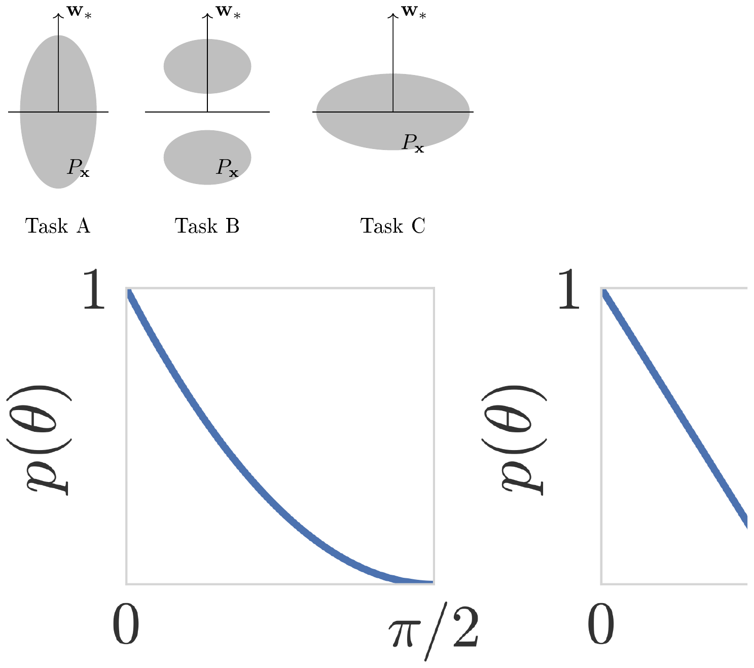
By construction, $p(\theta)$ is monotonically decreasing, starting with $p(0)=1$ and approaches $0$ for $\theta\to\pi/2$. Figure 1 illustrates this behavior for three exemplary data distributions as Tasks A, B and C. In Task A, the probability mass is well aligned with the direction of the teacher's weight vector. The probability that a randomly chosen data point $x\sim P_\mathbf x$ has a large angle with $\mathbf w_*$ is small. Therefore, the value of $p(\theta)$ quickly drops with growing angle $\theta$. In Task B, the data also aligns well with $\mathbf w_*$, but in addition, the data region remains bounded away from the decision boundary. Therefore, certain large angles can never occur, i.e. there exists a value $\theta_0<\pi/2$, such that $p(\theta)=0$ for $\theta\geq \theta_0$. In Task C, the situation is different: the data distribution is concentrated along the decision boundary and the probability of a angle between $\mathbf w_*$ and a randomly chosen data point $x\sim P_\mathbf x$ is large. As a consequence, $p(\theta)$ drops more slowly with growing angle than in the previous two settings.

We are now ready to state the main result. For improved readability, we phrase it for a student with infinitesimally small initialization, i.e. $\epsilon\to 0$. The general formulation can be found in the supplemental material.

########## {caption="Theorem 3: Transfer risk bound for linear distillation"}

For any training set $\mathbf X\in \mathbb R^{d\times n}$, let $\hat{h}\mathbf X(\mathbf x) = \mathbf{1}{\left{ \hat{\mathbf w}^\intercal \mathbf x \geq 0 \right}}$ be the linear classifier learned by distillation from a teacher with weight vector $\mathbf w*$. Then, when $n\geq d$, it holds that

$ \begin{aligned} \operatorname{\mathbb E}{\mathbf X\sim P\mathbf x^{\otimes n}}{\left[R\big(\hat{h}_\mathbf X \big) \right]} &= 0. \quad\text{(a)} \end{aligned} $

For $n<d$, it holds for any $\beta\in[0, \pi/2]$ that

$ \begin{aligned} \operatorname{\mathbb E}{\mathbf X\sim P\mathbf x^{\otimes n}}{\left[R\big(\hat{h}_\mathbf X \big) \right]} &\leq p(\beta) + p(\pi/2-\beta)^n \quad\text{(b)} \end{aligned}\tag{16} $

Equation 16a is unsurprising, of course, because in Section 4.1 we already established that for $n\geq d$ the student is able to perfectly mimic the teacher.

Inequality Equation 16b, however, is –to our knowledge– the first quantitative characterization how well a student can learn via distillation.

Before we provide the proof sketch, we present two instantiations of the bound for specific classes of tasks that provide insight how fast the right hand side of Equation 16b actually decreases.

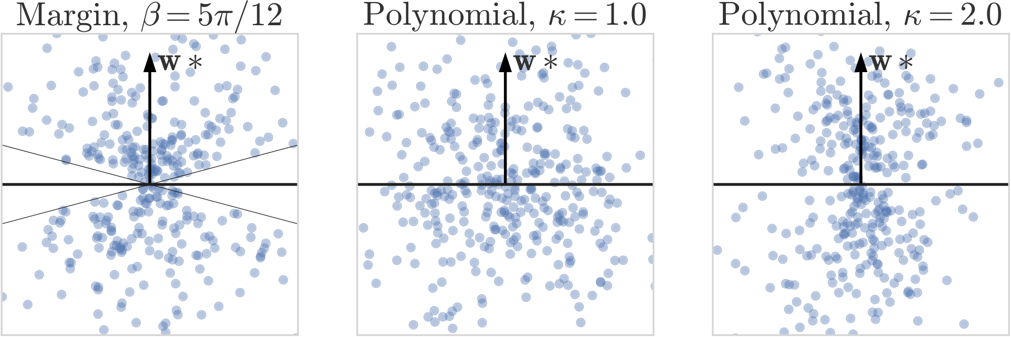
The margin case. The first class of tasks we consider are tasks in which the classes are separated by an angular margin, illustrated in Figure 2 (left). These tasks are characterized by a 'wedge' of zero probability mass near the boundary[^2]. For these tasks, we obtain from [@eq:bound] that the expected risk decays exponentially in $n$, up to $n=d-1$.

[^2]: In bounded domains this condition is, in particular, fulfilled in the classical margin situation [29], when the classes are separated by a positive distance from each other.

########## {caption="Corollary 4: Transfer risk of large-margin distributions"}

If there exists $\beta\in[0, \pi/2]$ such that $p(\beta)=0$ and $\gamma := p(\pi/2-\beta)<1$, then

$ \operatorname{\mathbb E}{\mathbf X\sim P\mathbf x^n}{\left[R\big(\hat{h}_\mathbf X \big) \right]} \leq \gamma^n.\tag{17} $

The polynomial case. The second class are tasks for which we can upper-bound $p$ by a $\kappa$-order polynomial. This can be done trivially for any task by setting $\kappa=0.0$, but that choice would yield a vacuous bound. Higher values of $\kappa$ correspond to stronger assumptions on the distribution but enable better rates. Figure 2 (center, right) shows examples of polynomial distributions for $\kappa\in{\left{ 1.0, 2.0 \right}}$. The special case $\kappa=1.0$ corresponds to a uniform angle distribution, while distribution with $\kappa=2.0$ have low probability mass near the decision boundary, while not necessarily exhibiting a margin.

The following corollary establishes that for tasks with polynomial behavior of $p(\theta)$, the expected risk decays essentially at a rate of $(\log n/n)^\kappa$ or faster.

########## {caption="Corollary 5: Transfer risk of polynomial distributions"}

If there exists a $\kappa\geq 0$ be such that $p(\theta) \leq c\cdot(1-(2/\pi)\theta)^\kappa$ for all $\theta\in[0, \pi/2]$, then

$ \operatorname{\mathbb E}{\mathbf X\sim P\mathbf x^n}{\left[R\big(\hat{h}_\mathbf X) \right]} \leq c\cdot\frac{1 + (\log n)^\kappa}{n^\kappa}\tag{18} $

Proof: We apply [@eq:bound] and insert the polynomial upper bound for $p$. For the case $n < d$, we get

$ \begin{aligned} & \operatorname{\mathbb E}{\mathbf X\sim P\mathbf x^n}{\left[R\big(\hat{h}_\mathbf X \big) \right]} \nonumber \ &\leq (1-(2/\pi)\beta)^\kappa + (1-(2/\pi)(\pi/2 - \beta))^{n\kappa}. \end{aligned} $

Setting $\beta = (\pi/2)\cdot n^{-1/n}$ and simplifying the resulting expressions yields

$ \begin{aligned} &\leq \big(1-e^{-\frac{\log n}{n}}\big)^\kappa + n^{-\kappa}. \end{aligned} $

Finally, we use the inequality $e^x \geq 1+x$ and the claim follows.

Note that, in contrast to many results in statistical learning theory, the bounds are far from vacuous, even when only little data is available. This can best be seen in Corollary 4, where $\gamma<1$ and hence $\gamma^n$ is an informative upper bound for the classification error. These observations suggest that distillation operates in a very different regime from classical hard-target learning. Standard bounds usually have little to say when $n<d$ and only start to be useful when $n\gg d$. In contrast, (linear) distillation ensures perfect transfer when $n\geq d$ and non-vacuous bounds are possible even when $n<d$.

4.3 Proof of

Theorem 3

The case $n\geq d$ follows trivially from the result of Theorem 1 and 2. For the case $n < d$, the following property turns out to be crucial for obtaining a transfer rate of the form that we do.

########## {caption="Lemma 6: Strong monotonicity"}

Let $\hat{\mathbf w}(\mathbf X)$ denote the distillation solution $\hat{\mathbf w}$ as a function of the training data $\mathbf X$. Then, for any full-rank datasets $\mathbf X_-\in \mathbb R^{d\times n_-}$ and $\mathbf X_+\in \mathbb R^{d\times n_+}$ such that $\mathbf X_-$ is contained in $\mathbf X_+$,

$ \bar\alpha(\mathbf w_*, \hat{\mathbf w}(\mathbf X_+)) \leq \bar\alpha(\mathbf w_*, \hat{\mathbf w}(\mathbf X_-)).\tag{19} $

Proof: If $n_+\geq d$, then the left-hand side of Equation (19) is zero and the claim follows. Otherwise, assume wlog that the first $n_-$ columns of $\mathbf X_-$ and $\mathbf X_+$ coincide. Let $\mathbf Q_+\mathbf R_+ = \mathbf X_+$ be the QR factorisation of $\mathbf X_+$ with $\mathbf Q_+\in \mathbb R^{d\times n_+}$ and $\mathbf R_+\in \mathbb R^{n_+\times n_+}$, and similarly for $\mathbf X_-$. Then $\hat{\mathbf w}(\mathbf X_+) = \mathbf Q_+\mathbf Q_+^\intercal \mathbf w_*$ and

$ \begin{aligned} \cos(\bar\alpha(\mathbf w_*, \hat{\mathbf w}(\mathbf X_+))) & = \frac{\mathbf w_* ^\intercal \mathbf Q_+\mathbf Q_+^\intercal \mathbf w_*} {{\left| \mathbf w_* \right|}\cdot{\left| \mathbf Q_+\mathbf Q_+^\intercal \mathbf w_* \right|}} \ & = \frac{{\left| \mathbf Q_+^\intercal \mathbf w_* \right|}} {{\left| \mathbf w_* \right|}}, \end{aligned} $

and an analogous statement holds for $\mathbf X_-$. Now, because the first $n_-$ columns of $\mathbf Q_+$ coincide with $\mathbf Q_-$, we have ${\left| \mathbf Q_+^\intercal \mathbf w_* \right|} \geq {\left| \mathbf Q_-^\intercal \mathbf w_* \right|}$ and

$ \cos(\bar\alpha(\mathbf w_*, \hat{\mathbf w}(\mathbf X_+))) \geq \cos(\bar\alpha(\mathbf w_*, \hat{\mathbf w}(\mathbf X_-))).\tag{20} $

Taking $\cos^{-1}$ on both sides (and remembering that $\cos^{-1}$ is decreasing) yields the claim.

For the moment, think of $\bar\alpha(\mathbf w_*, \hat{\mathbf w})$ as a proxy for the transfer risk, i.e. the closer the trained student $\hat{\mathbf w}$ is to the teacher $\mathbf w_*$ in terms of angles, the lower the transfer risk. A direct consequence of Lemma 6, and the reason we call it `strong mononoticity', is that including additional data in the transfer set can never harm the transfer risk, only improve it. This property is specific to distillation; it does not hold in hard-target learning.

Proof of [@eq:bound] $(n<d)$: For nonzero vectors $\mathbf u, \mathbf v \in \mathbb R^d$, we define $\alpha(\mathbf u, \mathbf v)\in[0, \pi]$ as a variant of $\bar\alpha$ Equation (14) that takes the sign of $\mathbf u ^\intercal \mathbf v$ into account,

$ \alpha(\mathbf u, \mathbf v) = \cos^{-1} {\left(\frac {{\mathbf u ^\intercal \mathbf v}} {{\left| \mathbf u \right|} \cdot {\left| \mathbf v \right|}} \right)}.\tag{21} $

We decompose the expected risk as follows:

$ \begin{aligned} \begin{split}\operatorname{\mathbb E}{\mathbf X\sim P\mathbf x^n}&{\left[R\big(\hat{h}\mathbf X \big) \right]} = \operatorname{\mathbb P}{\substack{\mathbf X\sim P_{\mathbf x}^n \ \mathbf x\sim P_{\mathbf x} }}[\mathbf w_* ^\intercal \mathbf x \cdot \hat{\mathbf w}^\intercal \mathbf x < 0]\&= \int_{\mathbf x: \bar\alpha(\mathbf w_*, \mathbf x) \geq \beta} \operatorname{\mathbb P}{\mathbf X\sim P{\mathbf x}^n}[\mathbf w_* ^\intercal \mathbf x\cdot \hat{\mathbf w}^\intercal \mathbf x <0 | \mathbf x], \mathrm{d}P_{\mathbf x}\&+ \int_{\mathbf x: \bar\alpha(\mathbf w_*, \mathbf x) < \beta, , \mathbf w_* ^\intercal \mathbf x > 0} \operatorname{\mathbb P}{\mathbf X\sim P{\mathbf x}^n}[\hat{\mathbf w}^\intercal \mathbf x <0 | \mathbf x], \mathrm{d}P_{\mathbf x}\&+ \int_{\mathbf x: \bar\alpha(\mathbf w_*, \mathbf x) < \beta, , \mathbf w_* ^\intercal \mathbf x < 0} \operatorname{\mathbb P}{\mathbf X\sim P_{\mathbf x}^n}[\hat{\mathbf w}^\intercal \mathbf x >0 | \mathbf x], \mathrm{d}P{\mathbf x} .\end{split} \end{aligned}\tag{22} $

Let us fix some $\mathbf x$ for which $\bar\alpha(\mathbf w_*, \mathbf x)<\beta$ and $\mathbf w_* ^\intercal \mathbf x > 0$ (i.e. an 'easy' positive test example); for this $\mathbf x$ we have $\alpha(\mathbf w_*, \mathbf x)=\bar\alpha(\mathbf w_*, \mathbf x)$. Consider the situation where $\bar\alpha(\mathbf w_*, \mathbf x_i)< \pi/2-\beta$ for some $i$ (i.e. there is at least one good teaching point). Then, Lemma 6 with $\mathbf X_+= \mathbf X$ and $\mathbf X_-= \mathbf x_i$ yields $\bar\alpha(\mathbf w_*, \hat{\mathbf w}) \leq \bar\alpha(\mathbf w_*, \mathbf x_i) < \pi/2 - \beta$. Combined with the triangle inequality, we obtain

$ \begin{aligned} \alpha(\hat{\mathbf w}, \mathbf x) &\leq \alpha(\mathbf w_*, \hat{\mathbf w}) + \alpha(\mathbf w_*, \mathbf x) \ &\leq \bar\alpha(\mathbf w_*, \mathbf x_i) + \bar\alpha(\mathbf w_*, \mathbf x) < \pi/2, \end{aligned} $

which implies $\hat{\mathbf w}^\intercal \mathbf x > 0$, i.e. a correct prediction (same as the teacher's). Conversely, an error can occur only if $\bar\alpha(\mathbf w_*, \mathbf x_i) \geq \pi/2 - \beta $ for all $i$. Because $\mathbf x_i$ are independent, we have

$ \begin{aligned} \begin{split}\operatorname{\mathbb P}{\mathbf X\sim P{\mathbf x}^n}[\hat{\mathbf w}^\intercal \mathbf x < &, 0 |, \mathbf x: \bar\alpha(\mathbf w_*, \mathbf x)<\beta, , \mathbf w_* ^\intercal \mathbf x>0]\&\leq \operatorname{\mathbb P}{\mathbf X\sim P{\mathbf x}^n}[\forall_i: \bar\alpha(\mathbf w_*, \mathbf x_i) \geq \pi/2 - \beta]\&= p(\pi/2-\beta)^n.\end{split} \end{aligned}\tag{23} $

By a symmetric argument, one can show that

$ \begin{split} \operatorname{\mathbb P}{\mathbf X\sim P{\mathbf x}^n}[\hat{\mathbf w}^\intercal \mathbf x >0 |, \mathbf x: \bar\alpha(\mathbf w_*, \mathbf x)<\beta, , \mathbf w_* ^\intercal \mathbf x<0] \ \leq p(\pi/2-\beta)^n. \end{split}\tag{24} $

Combining Equation (22), Equation (23) and (24) yields the result:

$ \begin{aligned} \operatorname{\mathbb P}{\substack{\mathbf X\sim P{\mathbf x}^n \ \mathbf x\sim P_{\mathbf x} }}&[\mathbf w_* ^\intercal \mathbf x \cdot \hat{\mathbf w}^\intercal \mathbf x < 0] \leq \ \leq&, \operatorname{\mathbb P}{\mathbf x}[\bar\alpha(\mathbf w, \mathbf x)\geq\beta] + \operatorname{\mathbb P}{\mathbf x}[\bar\alpha(\mathbf w, \mathbf x)<\beta] \cdot p(\pi/2-\beta)^n \ =&, p(\beta) + (1-p(\beta))\cdot p(\pi/2-\beta)^n. \end{aligned} $

5. Why Does Distillation Work?

Section Summary: Distillation succeeds primarily because of three intertwined factors: favorable data geometry that aligns training examples well with the teacher's decision boundary, an optimization bias from gradient descent that steers the student toward well-generalizing solutions among many equally good training minima, and strong monotonicity ensuring that adding more data steadily improves the student's approximation of the teacher. Experiments varying angular alignment, deliberately weakening gradient bias via random perturbations, and measuring how often extra examples reduce angle to the teacher confirm that each factor measurably lowers the student's transfer risk. Together they explain why distillation often outperforms training on hard labels even with limited data.

From the formal analysis in the previous section, three concepts emerge as key factors for the success of distillation: data geometry, optimization bias, and strong monotonicity. In this section, we discuss these factors and provide some empirical confirmation how they affect or explain variations in the transfer risk.

5.1 Data Geometry

From [@eq:bound] we know that the data geometry, in particular the angular alignment between the data distribution and the teacher, crucially impact how fast the student can learn. Formally, this is reflected in $p(\theta)$: the faster it decreases, the easier it should be for the student to learn the task.

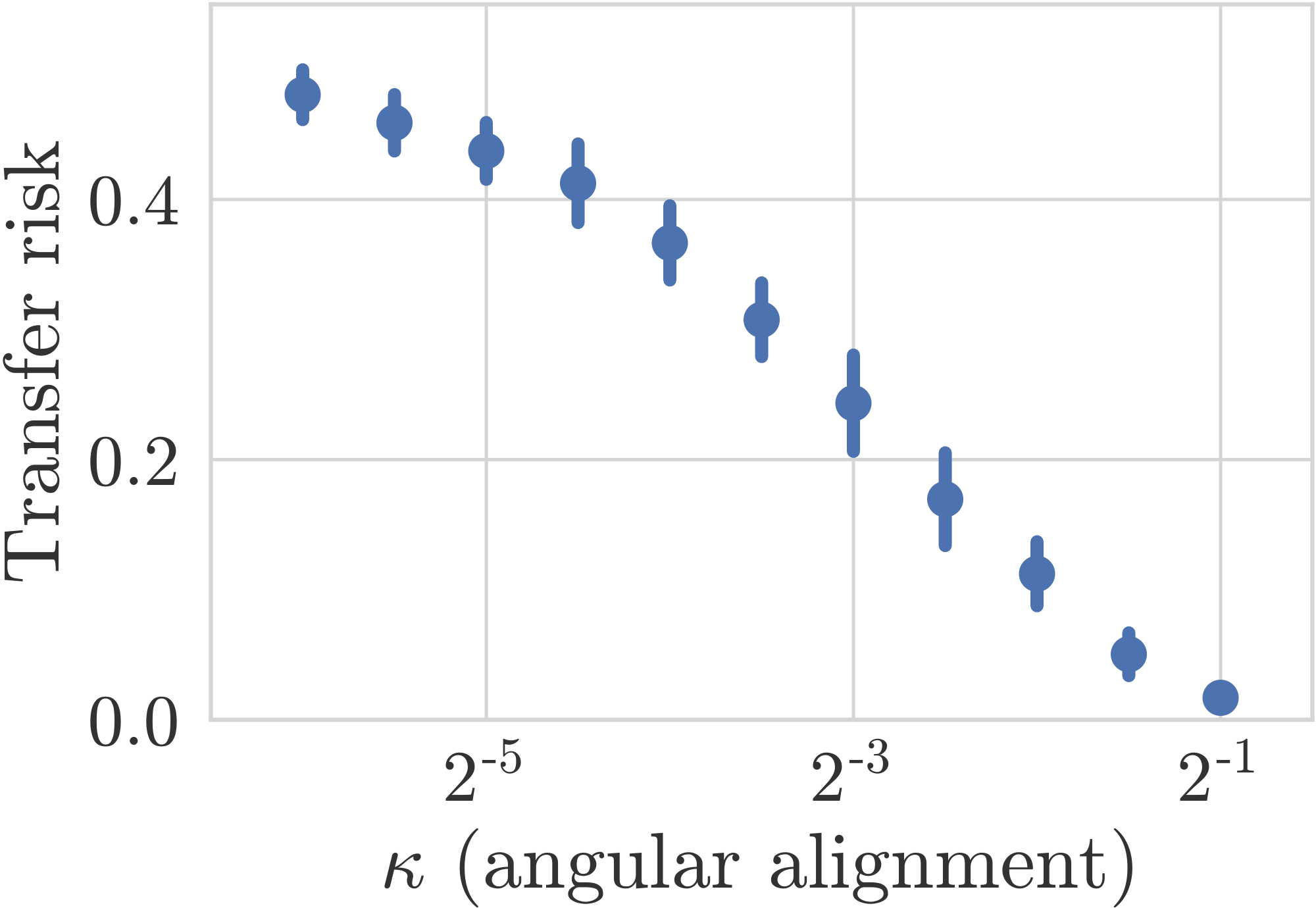
To experimentally test the effect of data geometry on the effectiveness of distillation, we adopt the setting of Corollary 5. We consider a series of tasks of varying angular alignment, as measured by the degree, $\kappa$, of the polynomial by which $p(\theta)$ is upper bounded.

Specifically, for any $\kappa$, the task $(P_\mathbf x^\kappa, \mathbf w_^\kappa)$ is defined by the following sampling procedure. First, an angle $a$ is sampled from the $\kappa$-polynomial distribution, i.e. $\operatorname{\mathbb P}{\left[a \geq \theta \right]} = (1-(2/\pi)\theta)^\kappa$ for $\theta\in[0, \pi/2]$. Then, a direction $\mathbf z$ is uniformly sampled from all unit-length vectors that are at angle $a$ with the teacher's weight vector, $\bar\alpha(\mathbf w_, \mathbf z) = a$. Finally, $\mathbf x = \nu \mathbf z$ is returned for a random $\nu$, distributed as a one-dimensional standard Gaussian.

We use an input space dimension of $d=1000$ and a transfer set size $n=20$. Then, we train a linear student by distillation on each of the tasks and evaluate its transfer risk on held-out data. Figure 3 shows the results. The plot shows a clearly decreasing trend: on tasks with more favorable data geometry (higher $\kappa$), transfer via distillation is more effective and the student achieves lower risk.

5.2 Optimization Bias

A second key factor for the success of distillation is a specific optimization bias. For $n<d$, the distillation training objective Equation 1 has many minima of identical function value but potentially different generalization properties. Therefore, the optimization method used could have a large impact on the transfer risk. As Theorem 1 and Theorem 2 show, gradient descent has a particularly favorable bias for distillation.

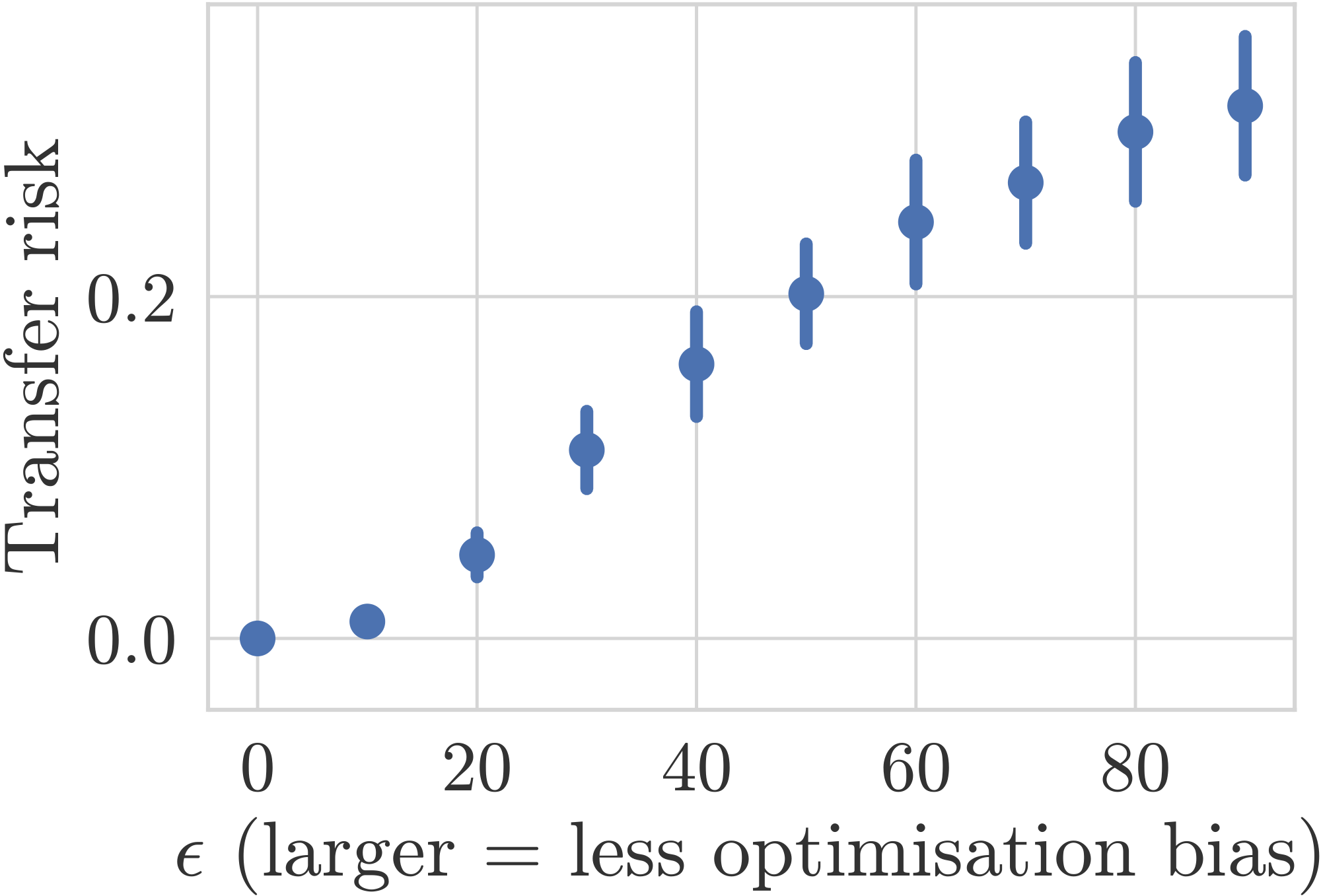
To verify this observation experimentally, we consider learners that are guided by an optimisation bias to different degrees: at one end of the spectrum is the gradient-descent learner we have studied in previous sections, while at the other end is a learner that treats all minimizers of the distillation training loss equally, i.e. that has no bias toward any of the solutions. Specifically, consider learners with weights of the form $\mathbf w_\delta = \hat{\mathbf w} + \delta\frac{{\left| \hat{\mathbf w} \right|}}{{\left| \mathbf q \right|}} \mathbf q$, where $\hat{\mathbf w}$ is the gradient-descent distillation solution and $\mathbf q$ is a Gaussian random vector in the subspace orthogonal to the data span, i.e. if $\mathbf X$ is the data matrix, then $\mathbf X ^\intercal \mathbf q = \mathbf{0}$. All learners of this form globally minimize the distillation training loss, and depending on $\delta$, they are more or less guided by the gradient-descent bias: $\delta=0$ and ${\left| \delta \right|} \to\infty$ represent the two extremes mentioned above.

We train the learners $\mathbf w_\delta$ for $\delta\in{\left{ 0, 10, \dots, 90 \right}}$ on the digits $0$ and $1$ of the MNIST dataset, where inputs are treated as vectors in $\mathbb R^{784}$ and the teacher $\mathbf w_*$ is a logistic regression trained to classify 0s and 1s on an independent training set. We set the transfer set size to $n=100$ and evaluate the risk on the test set.

Figure 4 shows the result. There is a clear trend in favor of learners that are more strongly guided by the gradient-descent bias (small $\delta$); these learners generally achieve lower transfer risk. This result supports the idea of optimization bias as a key component of distillation's success.

5.3 Strong Monotonicity

The third key factor we identify is strong monotonicity, as established in Lemma 6: training the student on more data always leads to a better approximation of the teacher's weight vector.

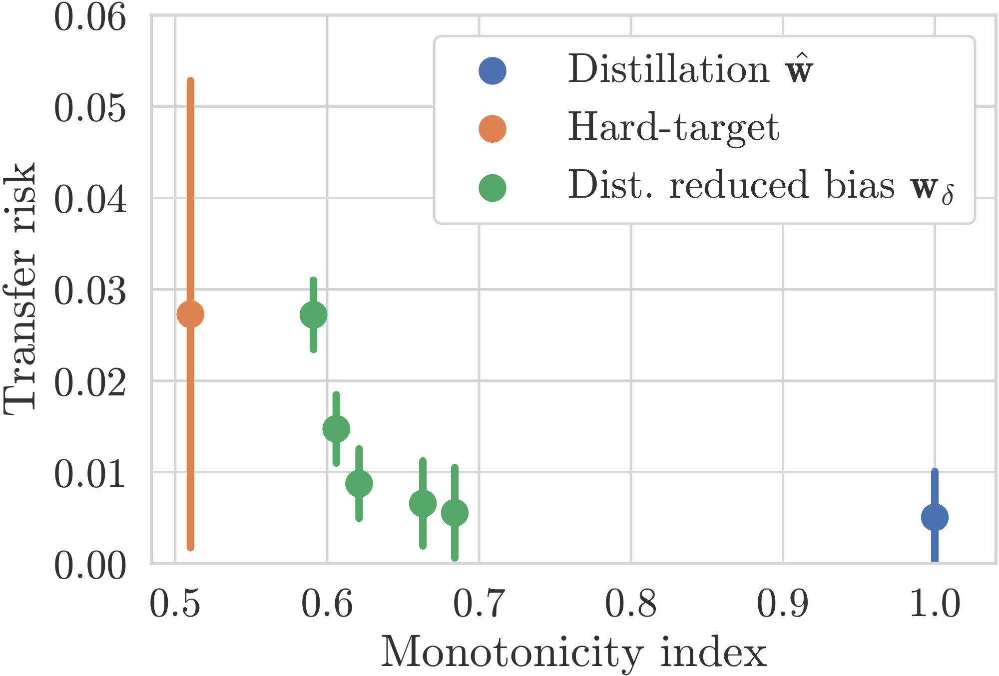
Compared to data geometry and optimisation bias, strong monotonicity is less amenable to experimental study because it is a downstream property that cannot directly be manipulated. We therefore take an indirect approach. We consider a set of learners including the gradient-descent distillation learner, the hard-target learner, and several learners with reduced optimisation bias (as in Section 5.2), and train them on the same task. For each learner, we note its expected risk calculated on a held-out set, and its monotonicity index, defined as the probability that an additional training example reduces the angle between the student's and the teacher's weight vectors rather than increasing it, i.e.

$ m(\mathbf w) = \operatorname{\mathbb P}{\substack{ \mathbf X\sim P\mathbf x^n \ \mathbf x\sim P_\mathbf x}} {\left[\bar\alpha(\mathbf w_*, \mathbf w([\mathbf X, \mathbf x])) < \bar\alpha(\mathbf w_*, \mathbf w(\mathbf X)) \right]},\tag{25} $

where the student's weight vector $\mathbf w$ is now treated as a function of the training set. Thus, we can relate a learner's risk and its monotonicity.

We train the learners on the polynomial-angle task $(P_\mathbf x^\kappa, \mathbf w_*^\kappa)$ from Section 5.1, with $\kappa=1, d=100$ and $n=5$. The expected risk as well as the monotonicity index are estimated as averages over 1000 transfer sets.

The results are shown in Figure 5. There is a negative correlation between monotonicity and transfer risk, which supports the intuition of monotonicity as a desirable property and a possible explanation of distillation's success.

However, a few reservations are in order. First, as mentioned above, monotonicity cannot easily be manipulated, so its effect on transfer risk remains unknown. We can only measure correlation. Second, monotonicity is of binary nature; it only captures whether an extra data point helps or not. Yet for a quantitative characterization of risk, one would have to capture by how much an extra data point helps. We leave more refined definitions of monotonicity for future work.

6. Conclusion

Section Summary: In this work the authors developed a simplified linear model of knowledge distillation and used it to characterize what the student learns, bound its risk even with limited data, and identify the main reasons distillation succeeds. They show that gradient methods started near the origin naturally produce a student that closely mimics the teacher and improves with every added example, with further gains from favorable spacing between classes. Although these results are proven only for linear models, the authors suggest the same mechanisms likely operate in deeper networks and could guide the design of smaller transfer datasets or more efficient learning algorithms.

In this work, we have formulated and studied a linear model of knowledge distillation. Within this model, we have derived a) a characterization of the solution learned by the student, b) a bound on the transfer risk, meaningful even in the low-data regime, and c) three key factors that explain the success of distillation. In doing so, we hope to have enriched both the current intuitive and theoretical understanding of distillation, both of which have only been weakly developed.

Our work paints a picture of distillation as an extremely effective method for knowledge transfer that derives its power from an optimization bias of gradient-based methods initialized near the origin, which in particular has the effect that any additionally included training point can only improve the student's approximation of the teacher. Distillation further benefits strongly from a favorable data geometry, in particular a margin between classes.

While we have supported this picture by theory and empirical work only in the linear case, we hypothesize that similar properties also govern the behavior of distillation in the nonlinear setting. If this hypothesis turns out to be true, it would have implications for the design of transfer sets (a large teacher model being stored along with only the minimal dataset necessary for future transfer) or active learning (which samples are most informative to have labeled by the teacher). Potentially, strong monotonicity could serve as a leading design principle for new sample-efficient algorithms. We thus consider the extension to nonlinear models the main direction for future work.

Appendix

Section Summary: The appendix introduces extra notation beyond the main paper for studying a neural network training objective based on cross-entropy, including a normalized per-example loss ℓ_i and the projection matrix onto the column span of any full-rank matrix. It then states and proves three key properties of this loss: an explicit formula for its gradient (which always lies in the span of the data matrix), a characterization of its global minimizers, and a restricted strong-convexity bound that holds inside any sublevel set when movement is confined to the data span. These results rely on Taylor expansion of the loss together with bounds on the logistic function inside bounded regions.

numberwithinassumptionsection numberwithincorollarysection numberwithinlemmasection numberwithintheoremsection

We define here some notation in addition to that of Section 3 in the main text. We denote by $\ell_i$ the per-instance loss,

$ \begin{aligned} L^1(\mathbf w) &= \frac 1 n \sum_{i=1}^n \ell_i(\mathbf w ^\intercal \mathbf x_i), \ \ell_i(u) &= -y_i\log\sigma(u) - (1-y_i)\log(1-\sigma(u)) - \ell_i^*, \end{aligned}\tag{26} $

where $\ell_i^*$ are constants chosen such that the minimum of $\ell_i$ is 0, namely $\ell_i^* = - y_i\log y_i - (1-y_i)\log(1-y_i)$.

Slightly abusing notation, we write $L(\tau) = L^1(\mathbf w(\tau)) = L(\mathbf W_1(\tau), \dots, \mathbf W_N(\tau)) $ for the objective value at time $\tau$.

Finally, for a full-rank matrix $\mathbf A\in \mathbb R^{d\times m}\ (m\geq 1)$, we denote by $\mathbf P_\mathbf A\in \mathbb R^{d\times d}$ the matrix of projection onto the span of $\mathbf A$,

$ \mathbf P_\mathbf A = \left{ \begin{array}{cl} \mathbf I, & m\geq d, \ \mathbf A(\mathbf A ^\intercal \mathbf A)^{-1}\mathbf A ^\intercal, & m < d. \end{array}\right.\tag{27} $

A. Properties of the Cross-Entropy Loss

########## {caption="Theorem 7: Gradient"}

The gradient of the cross-entropy loss Equation (26) takes the form

$ \nabla L^1(\mathbf w) = \frac 1 n \sum_{i=1}^n (\sigma(\mathbf w ^\intercal \mathbf x_i)-y_i) \cdot \mathbf x_i.\tag{28} $

It always lies in the data span, $\nabla L^1(\mathbf w) \in \mathrm{span}(\mathbf X)$.

Proof: Straightforward calculation.

########## {caption="Theorem 8: Global minima"}

The global minimum of the cross-entropy loss Equation (26) is 0 and the set of global minimisers is

$ {\left{ \mathbf w\in \mathbb R^d: \mathbf X ^\intercal \mathbf w = \mathbf X ^\intercal \mathbf w_* \right}}.\tag{29} $

Proof: We know that $L^1\geq 0$ and $L^1(\mathbf w_*)=0$, so 0 is the optimal objective value, and the set of global optima consists of all $\mathbf w$ such that $L^1(\mathbf w)=0$. The last condition is equivalent to $\forall_i: \ell_i(\mathbf w)=0$, which in turn is equivalent to $\forall_i: \sigma(\mathbf w ^\intercal \mathbf x_i) = \sigma(\mathbf w_* ^\intercal \mathbf x_i)$. By monotonicity of $\sigma$, this is further equivalent to $\forall_i: \mathbf w ^\intercal \mathbf x_i = \mathbf w_* ^\intercal \mathbf x_i$, which is a restatement of Equation (29).

########## {caption="Theorem 9: Restricted strong convexity"}

Assume $\mathbf X$ is full-rank. For any sublevel set $\mathcal W={\left{ \mathbf w: L^1(\mathbf w)\leq l \right}}$, there exists $\mu>0$ such that

$ \begin{split} L^1(\mathbf v) \geq L^1(\mathbf w) + \nabla L^1(\mathbf w)^\intercal(\mathbf v-\mathbf w)

• \frac \mu 2 {\left| \mathbf v-\mathbf w \right|}^2 \end{split}\tag{30} $

for all $\mathbf w, \mathbf v\in \mathcal W$ such that $\mathbf v-\mathbf w\in\mathrm{span}(\mathbf X)$.

Proof: Consider the 2nd-order Taylor expansion of $L^1$ around $\mathbf w$,

$ \begin{split} L^1(\mathbf v) = L^1(\mathbf w) + \nabla L^1(\mathbf w)^\intercal(\mathbf v - \mathbf w) \

• \frac 1 2(\mathbf v - \mathbf w)^\intercal [\nabla^2L^1(\bar{\mathbf w})] (\mathbf v - \mathbf w), \end{split}\tag{31} $

where $\nabla^2L^1(\bar{\mathbf w})$ is the Hessian of $L^1$ evaluated at $\bar{\mathbf w}$, a point lying between $\mathbf v$ and $\mathbf w$. A straightforward calculation shows that the Hessian takes the form

$ \nabla^2 L^1(\bar{\mathbf w}) = \mathbf X \mathbf D_{\bar{\mathbf w}}\mathbf X ^\intercal,\tag{32} $

where

$ \begin{split} \mathbf D_{\bar{\mathbf w}} = \mathrm{diag}[\sigma(\bar{\mathbf w}^\intercal \mathbf x_1)(1-\sigma(\bar{\mathbf w}^\intercal \mathbf x_1)), \ \dots, \sigma(\bar{\mathbf w}^\intercal \mathbf x_n)(1-\sigma(\bar{\mathbf w}^\intercal \mathbf x_n))]. \end{split} $

We will now show that there is a constant $\omega>0$ such that

$ \sigma(\bar{\mathbf w}^\intercal \mathbf x_i)(1 - \sigma(\bar{\mathbf w}^\intercal \mathbf x_i)) \geq \omega\tag{33} $

for all $\bar{\mathbf w}\in \mathcal W$ and $i\in{\left{ 1, \dots, n \right}}$, so that we can claim $\mathbf D_{\bar{\mathbf w}}\succeq \omega \mathbf I$, or consequently $\nabla^2 L^1(\bar{\mathbf w}) \succeq \omega \mathbf X \mathbf X ^\intercal$.

Let $\mathbf w\in \mathcal W$. The bound on $L^1(\mathbf w)$ implies a bound on $\ell_i(\mathbf w ^\intercal \mathbf x_i)$ for all $i$,

$ \ell_i(\mathbf w ^\intercal \mathbf x_i) \leq nL^1(\mathbf w) \leq nl.\tag{34} $

Because $\ell_i$ is convex and $\ell_i(u)\to\infty$ as $u\to\pm\infty$, we know that $\ell_i^{-1}((-\infty, nl])$ is a bounded interval, and the finite union $\cup_{i=1}^n \ell_i^{-1}((-\infty, nl])$ is also a bounded interval, whose size depends only on $nl$ and the data. Hence, there exists $K>0$ such that $\mathbf w ^\intercal \mathbf x_i \in [-K, K]$ for all $\mathbf w\in \mathcal W$ and $i\in{\left{ 1, \dots, n \right}}$. The existence of $\omega>0$ satisfying Equation (33) follows.

Now, let us apply $\nabla^2L^1(\mathbf w)\succeq \omega \mathbf X \mathbf X ^\intercal$ to lower-bound Equation (31):

$ \begin{split} L^1(\mathbf v) \geq L^1(\mathbf w) + \nabla L^1(\mathbf w)^\intercal(\mathbf v-\mathbf w) \

• \frac \omega 2 (\mathbf v - \mathbf w)^\intercal \mathbf X \mathbf X ^\intercal(\mathbf v - \mathbf w). \end{split}\tag{35} $

Consider two cases. If $n\geq d$, $\mathbf X \mathbf X ^\intercal$ is full-rank and $\mathbf X \mathbf X ^\intercal \succeq \lambda_\mathrm{min}\mathbf I$ holds, where $\lambda_\mathrm{min}>0$ is the smallest eigenvalue of $\mathbf X \mathbf X ^\intercal$. Combined with Equation (35), this proves the claim for $n\geq d$ and $\mu=\omega\lambda_\mathrm{min}$.

If $n<d$, $\mathbf X ^\intercal \mathbf X$ is full rank. We can use the assumption $\mathbf v-\mathbf w\in\mathrm{span}(\mathbf X)$ to deduce

$ \begin{aligned} \begin{split}{\left| \mathbf v-\mathbf w \right|}^2 &= {\left| \mathbf P_\mathbf X(\mathbf v-\mathbf w) \right|}^2\&= (\mathbf v-\mathbf w)^\intercal \mathbf X(\mathbf X ^\intercal \mathbf X)^{-1}\mathbf X ^\intercal (\mathbf v-\mathbf w)\&\leq \lambda_\mathrm{max} (\mathbf v-\mathbf w)^\intercal \mathbf X \mathbf X ^\intercal(\mathbf v-\mathbf w), \end{split} \end{aligned} $

where $\lambda_\mathrm{max}>0$ is the largest eigenvalue of $(\mathbf X ^\intercal \mathbf X)^{-1}$. Combined with Equation (35), this proves the claim for $n<d$ and $\mu=\omega/\lambda_\mathrm{max}$.

########## {caption="Corollary 10: Restricted Polyak-Lojasiewicz"}

Assume $\mathbf X$ is full-rank. For any sublevel set $\mathcal W = {\left{ \mathbf w: L^1(\mathbf w)\leq l \right}}$, there exists $c>0$ such that

$ cL^1(\mathbf w) \leq \frac 1 2 {\left| \nabla L^1(\mathbf w) \right|}^2\tag{36} $

for all $\mathbf w\in \mathcal W$.

Proof: Let $\mathbf w\in \mathcal W$. (If $\mathcal W$ is empty, the claim is trivially true.) Equation 9 applied to $\mathcal W$ implies that for some $\mu>0$,

$ L^1(\mathbf v) \geq L^1(\mathbf w) + \nabla L^1(\mathbf w)^\intercal(\mathbf v-\mathbf w)

• \frac {\mu} 2 {\left| \mathbf v-\mathbf w \right|}^2\tag{37} $

for all $\mathbf v\in \mathcal W\cap \mathcal V$ where $\mathcal V = {\left{ \mathbf v: \mathbf v-\mathbf w\in\mathrm{span}(\mathbf X) \right}}$. Taking $\min_{\mathbf v\in \mathcal W\cap \mathcal V}$ on both sides, then relaxing part of the constraint on the right-hand side yields

$ \begin{aligned} \begin{split}&\min_{\mathbf v\in \mathcal W\cap \mathcal V} L^1(\mathbf v)\& \geq \min_{\mathbf v\in \mathcal W\cap \mathcal V} L^1(\mathbf w) + \nabla L^1(\mathbf w)^\intercal(\mathbf v-\mathbf w) + \frac \mu 2 {\left| \mathbf v -\mathbf w \right|}^2\& \geq \min_{\mathbf v\in \mathcal V} L^1(\mathbf w) + \nabla L^1(\mathbf w)^\intercal(\mathbf v-\mathbf w) + \frac \mu 2 {\left| \mathbf v -\mathbf w \right|}^2.\end{split} \end{aligned} $

Now, the minimum on the left-hand side is equal to 0 and is attained at $\mathbf v = \mathbf w + \mathbf P_\mathbf X(\mathbf w_* - \mathbf w)$, as can be seen from Theorem 8. For the right-hand side, we can substitute $\mathbf v = \mathbf w + \mathbf X \mathbf a$ for $\mathbf a\in \mathbb R^n$ and find the unconstrained minimum with respect to $\mathbf a$. We get

$ \begin{aligned} \begin{split} 0 &\geq L^1(\mathbf w) - \frac 1 {2\mu} \nabla L^1(\mathbf w)^\intercal \mathbf X(\mathbf X ^\intercal \mathbf X)^{-1}\mathbf X ^\intercal\nabla L^1(\mathbf w) \ &\geq L^1(\mathbf w) - \frac {\lambda_\mathrm{max}} {2\mu} {\left| \nabla L^1(\mathbf w) \right|}^2, \end{split} \end{aligned} $

where $\lambda_\mathrm{max}>0$ is the largest eigenvalue of $\mathbf X(\mathbf X ^\intercal \mathbf X)^{-1}\mathbf X ^\intercal$. This yields the result with $c=\mu/\lambda_\mathrm{max}$.

B. Proof of Theorem 1

We will prove a supporting lemma, and then the theorem.

########## {caption="Lemma 11"}

Assume the student is a directly parameterised linear classifier $(N=1)$ initialised at zero, $\mathbf w(0)=\mathbf{0}$. Then, $\mathbf w(\tau) \in\mathrm{span}(\mathbf X)$ for $\tau\in[0, \infty)$.

Proof: Let $\mathbf q\in \mathbb R^d$ be any vector orthogonal to the span of $\mathbf X$. It suffices to show that $\mathbf q ^\intercal \mathbf w(\tau) = 0$. For that, notice that $\mathbf q ^\intercal \mathbf w(0) = 0$ and

$ {\frac{\mathrm{d} }{\mathrm{d} \tau}} (\mathbf q ^\intercal \mathbf w(\tau)) = -\mathbf q ^\intercal\nabla L^1(\mathbf w(\tau)) = 0,\tag{38} $

where the last equality follows from the fact that $\nabla L^1(\mathbf w(\tau))\in\mathrm{span}(\mathbf X)$ (Theorem 7). The claim follows.

Proof: Recall the time-derivative of $L$,

$ L'(\tau) = -{\left| \nabla L^1(\mathbf w(\tau)) \right|}^2.\tag{39} $

The data matrix $\mathbf X$ is almost surely (wrt. $\mathbf X\sim P_\mathbf x^n$) full-rank, we can therefore apply Corollary 10 to $\mathcal W = {\left{ \mathbf w: L^1(\mathbf w)\leq L^1(\mathbf{0}) \right}}$ and $\mathbf w(\tau)$ to lower-bound the gradient norm on the right-hand side of Equation (39). We obtain $L'(\tau) \leq -cL(\tau)$ for some $c>0$ and all $\tau\in[0, \infty)$, or equivalently,

$ (\log L(\tau))' \leq -c. $

Integrating over $[0, t]$ yields $L(t) \leq L(0)\cdot e^{-ct}$, which proves global convergence in the objective: $L(t)\to 0$ as $t\to\infty$.

Now invoke Equation 9 with $\mathcal W$ as above, $\mathbf v= \mathbf w(t)$ and $\mathbf w=\hat{\mathbf w}$ (we know that both $\mathbf w(\tau), \hat{\mathbf w}\in \mathcal W\cap\mathrm{span}(\mathbf X)$, partly by Lemma 11):

$ L(t) \geq \frac\mu 2 {\left| \mathbf w(t) - \hat{\mathbf w} \right|}^2.\tag{40} $

Since $L(t)\to 0$ as $t\to\infty$, the theorem follows.

C. Proof of Theorem 2

For the proof, we will need a result by [27], which characterises the induced flow on $\mathbf w(\tau)$ when running gradient descent on the component matrices $\mathbf W_i$.

########## {caption="Lemma 12: {([27], Claim 2)}"}

If the balancedness condition Equation (11c) holds, then

$ \begin{split} {\frac{\partial \mathbf w(\tau)}{\partial \tau}} = -{\left| \mathbf w(\tau) \right|}^{\frac{2(N-1)}{N}} \left(\nabla L^1(\mathbf w(\tau)) + \right. \ \left. (N-1)\cdot \mathbf P_{\mathbf w(\tau)} \nabla L^1(\mathbf w(\tau)) \right). \end{split} $

Proof of Theorem 2: Similarly to the case $N=1$, we start by looking at the time-derivative of $L$,

$ \begin{aligned} \begin{split}L'(\tau) =& \nabla L^1(\mathbf w(\tau))^\intercal{\left({\frac{\partial \mathbf w(\tau)}{\partial \tau}} \right)}\=& -{\left| \mathbf w(\tau) \right|}^{\frac{2(N-1)}{N}} \left({\left| \nabla L^1(\mathbf w(\tau)) \right|}^2 \right.\& \left. + (N-1)\cdot {\left| \mathbf P_{\mathbf w(\tau)}\nabla L^1(\mathbf w(\tau)) \right|}^2 \right)\\leq & -{\left| \mathbf w(\tau) \right|}^{\frac{2(N-1)}{N}} \cdot {\left| \nabla L^1(\mathbf w(\tau)) \right|}^2 .\end{split} \end{aligned}\tag{41} $

It is non-positive, so $\mathbf w(\tau)$ stays within the $L(0)$-sublevel set throughout optimisation,

$ \mathbf w(\tau)\in \mathcal W = {\left{ \mathbf w: L^1(\mathbf w)\leq L(0) \right}}.\tag{42} $

Also, $\mathcal W$ is convex and by Assumption (11b) it does not contain $\mathbf{0}$. We can therefore take $\delta > 0$ to be the distance between $\mathcal W$ and $\mathbf{0}$, and it follows that ${\left| \mathbf w(\tau) \right|}\geq\delta$ for $\tau\in[0, \infty)$.

Now, noting that $\mathbf X$ is almost surely full-rank, apply Corollary 10 to $\mathcal W$ and $\mathbf w(\tau)$ to upper-bound the right-hand side of Equation (41),

$ L'(\tau) \leq - c\delta^{\frac{2(N-1)}{N}} L(\tau).\tag{43} $

Letting $\tilde{c} = c\delta^{\frac{2(N-1)}{N}}$, we get $(\log L(\tau))' \leq -\tilde{c}$ and consequently $L(t)\leq L(0)\cdot e^{-\tilde{c} t}$. This proves convergence in the objective, $L(t)\to 0$ as $t\to\infty$.

To prove convergence in parameters, we decompose the 'error' $\mathbf w(\tau) - \hat{\mathbf w}$ into orthogonal components and bound each of them separately,

$ \begin{split} {\left| \mathbf w(\tau) - \hat{\mathbf w} \right|}^2 = {\left| \mathbf P_\mathbf X(\mathbf w(\tau)-\hat{\mathbf w}) \right|}^2 \ + {\left| \mathbf P_\mathbf Q(\mathbf w(\tau)-\hat{\mathbf w}) \right|}^2, \end{split}\tag{44} $

where the columns of $\mathbf Q\in \mathbb R^{d\times(d-n)}$ orthogonally complement those of $\mathbf X$. If $n\geq d$, we simply bound the first term and disregard the second one.

To bound the first term, invoke Equation 9 with $\mathcal W$, $\mathbf v= \mathbf P_\mathbf X \mathbf w(\tau)$ and $\mathbf w= \mathbf P_\mathbf X\hat{\mathbf w}$. One can check that $L^1(\mathbf P_\mathbf X \mathbf u) = L^1(\mathbf u)$ for all $\mathbf u\in \mathbb R^d$, so $\mathbf P_\mathbf X \mathbf w(\tau)\in \mathcal W$ and our use of the theorem is legal. We obtain

$ L(\tau) \geq \frac \mu 2 {\left| \mathbf P_\mathbf X(\mathbf w(\tau) - \hat{\mathbf w}) \right|}^2.\tag{45} $

Since $L(\tau)\to 0$, it follows that

$ {\left| \mathbf P_\mathbf X(\mathbf w(\tau) - \hat{\mathbf w}) \right|}^2\to 0\tag{46} $

as $\tau\to\infty$.

For the second term, notice that $\hat{\mathbf w}\in\mathrm{span}(\mathbf X)$, so $\mathbf P_\mathbf Q\hat{\mathbf w}$ vanishes and we are left with ${\left| \mathbf P_\mathbf Q \mathbf w(\tau) \right|}^2$. Denote this quantity $q(\tau)$. Its time derivative is

$ \begin{aligned} \begin{split}q'(\tau) =& \ 2(\mathbf P_\mathbf Q \mathbf w(\tau))^\intercal{\left({\frac{\partial \mathbf w(\tau)}{\partial \tau}} \right)}\=& -2{\left| \mathbf w(\tau) \right|}^{\frac{2(N-1)}N} \bigg(\mathbf w(\tau)^\intercal \mathbf P_\mathbf Q \nabla L^1(\mathbf w(\tau)) +\& \frac{(N-1)}{{\left| \mathbf w(\tau) \right|}^2}\cdot \mathbf w(\tau)^\intercal \mathbf P_\mathbf Q \mathbf w(\tau) \cdot \mathbf w(\tau)^\intercal \nabla L^1(\mathbf w(\tau)) \bigg)\=& -2q(\tau) (N-1) {\left| \mathbf w(\tau) \right|}^{-2/N} \mathbf w(\tau)^\intercal\nabla L^1(\mathbf w(\tau)), \end{split} \end{aligned} $

where we have used the fact that $\nabla L^1(\mathbf w(\tau))\in\mathrm{span}(\mathbf X)$ (Theorem 7) and $\mathbf Q$ is orthogonal to $\mathbf X$. Rearranging, we obtain

$ {\frac{\mathrm{d} }{\mathrm{d} \tau}}{\left(\frac{\log q(\tau)}{2(N-1)} \right)} = -{\left| \mathbf w(\tau) \right|}^{-2/N}\cdot \mathbf w(\tau)^\intercal \nabla L^1(\mathbf w(\tau)).\tag{47} $

It turns out that the right-hand side expression is integrable in yet another way, namely

$ \begin{split} {\frac{\mathrm{d} }{\mathrm{d} \tau}}{\left(\frac 1 2N \log {\left| \mathbf w(\tau) \right|}^2 \right)} = \ -{\left| \mathbf w(\tau) \right|}^{-2/N}\cdot \mathbf w(\tau)^\intercal \nabla L^1(\mathbf w(\tau)). \end{split} $

Equating the two and integrating over $[0, t]$ yields

$ \log\frac{q(t)}{q(0)} = \frac{N-1}N \cdot \log\frac{{\left| \mathbf w(t) \right|}^2}{{\left| \mathbf w(0) \right|}^2},\tag{48} $

which implies

$ \frac{q(t)}{{\left| \mathbf w(t) \right|}^2} \leq {\left(\frac{{\left| \mathbf w(0) \right|}}{{\left| \mathbf w(t) \right|}} \right)}^{2/N},\tag{49} $

because $q(0)\leq {\left| \mathbf w(0) \right|}^2$.

We now bound the norm of $\mathbf w(t)$. Starting from an orthogonal decomposition similar to (44) and applying Equation (46) with Equation (49), we get

$ \begin{aligned} \begin{split} {\left| \mathbf w(t) \right|}^2 = & {\left| \mathbf P_\mathbf X \mathbf w(t) \right|}^2 + {\left| \mathbf P_\mathbf Q \mathbf w(t) \right|}^2 \ \limsup_{t\to\infty}{\left| \mathbf w(t) \right|}^2 \leq & {\left| \hat{\mathbf w} \right|}^2 + {\left| \mathbf w(0) \right|}^{\frac 2 N} \limsup_{t\to\infty} {\left| \mathbf w(t) \right|}^{2-\frac{2}N}. \end{split} \end{aligned} $

Denote $\nu:=\limsup_{t\to\infty} {\left| \mathbf w(t) \right|}$. By the same orthogonal decomposition, we also know that $\nu^2 \geq \limsup_{t\to\infty} {\left| \mathbf P_\mathbf X \mathbf w(t) \right|}^2={\left| \hat{\mathbf w} \right|}^2 > 0$, so we can divide both sides above by $\nu^2$,

$ 1 \leq \frac{{\left| \hat{\mathbf w} \right|}^2}{\nu^2} + \frac{{\left| \mathbf w(0) \right|}^{2/N} }{\nu^{2/N}} =: f(\nu).\tag{50} $

On the right-hand side, we now have a decreasing function of $\nu$ that goes to zero as $\nu\to\infty$. However, evaluated at our specific $\nu$, it is lower-bounded by $1$, implying an implicit upper bound for $\nu$.

How do we find this bound? Suppose we find some constant $K$ such that $f(K)\leq 1$. Then, because $f$ is decreasing, it must be the case that $\nu\leq K$. One such candidate for $K$ is

$ K = {\left| \hat{\mathbf w} \right|}\cdot {\left(1 - \frac{{\left| \mathbf w(0) \right|}^{2/N}}{{\left| \hat{\mathbf w} \right|}^{2/N}} \right)} ^{\frac{-N}{2(N-1)}}.\tag{51} $

(Here we have used condition Equation (11a): ${\left| \mathbf w(0) \right|} < {\left| \hat{\mathbf w} \right|}$.) To check that indeed $f(K)\leq 1$, start from the inequality

$ \begin{split} {\left({{\left| \hat{\mathbf w} \right|}} /K \right)}^{\frac{2(N-1)}N} + \frac{{\left| \mathbf w(0) \right|}^{2/N}}{{\left| \hat{\mathbf w} \right|}^{2/N}} = 1 \ \leq {\left(1 - \frac{{\left| \mathbf w(0) \right|}^{2/N}}{{\left| \hat{\mathbf w} \right|}^{2/N}} \right)}^{\frac{-1}{N-1}} = ({\left| \hat{\mathbf w} \right|} / K)^{-\frac 2 N}. \end{split} $

Taking the leftmost and rightmost expression and multiplying by $({\left| \hat{\mathbf w} \right|}/K)^{2/N}$ yields

$ f(K) = \frac{{\left| \hat{\mathbf w} \right|}^2} {K^{2}} + \frac{{\left| \mathbf w(0) \right|}^{2/N}}{K^{2/N}} \leq 1.\tag{52} $

Hence,

$ \limsup_{t\to\infty} {\left| \mathbf w(t) \right|} \leq {\left| \hat{\mathbf w} \right|}\cdot {\left(1 - \frac{{\left| \mathbf w(0) \right|}^{2/N}}{{\left| \hat{\mathbf w} \right|}^{2/N}} \right)} ^{\frac{-N}{2(N-1)}}.\tag{53} $

Finally, let us turn back to our original goal of bounding ${\left| \mathbf w(\tau) - \hat{\mathbf w} \right|}^2$. With Equation (44), Equation (46), Equation (49) and (53), we now know that

$ \begin{aligned} &\limsup_{t\to\infty} {\left| \mathbf w(\tau) - \hat{\mathbf w} \right|}^2 \ & \leq {\left| \mathbf w(0) \right|}^{\frac 2 N} {\left| \hat{\mathbf w} \right|}^{\frac{2(N-1)}{N}} {\left(1 - \frac{{\left| \mathbf w(0) \right|}^{\frac 2N}}{{\left| \hat{\mathbf w} \right|}^{\frac 2N}} \right)} ^{-1} \ &= \frac{{\left| \hat{\mathbf w} \right|}^{2+2/N}}{{\left| \hat{\mathbf w} \right|}^{2/N} - {\left| \mathbf w(0) \right|}^{2/N} } - {\left| \hat{\mathbf w} \right|}^2. \end{aligned} $

Hence, if we initialise close enough to zero, as specified by condition Equation (11a), we can ensure that

$ \limsup_{t\to\infty} {\left| \mathbf w(\tau)-\hat{\mathbf w} \right|}^2 < \epsilon^2.\tag{54} $

This concludes the proof.

D. [@eq:bound] for Approximate Distillation

We extend [@eq:bound] to the setting where the student learns the solution $\hat{\mathbf w} = \mathbf X(\mathbf X ^\intercal \mathbf X)^{-1}\mathbf X ^\intercal \mathbf w_*$ only $\epsilon$-approximately, as is the case for deep linear networks initialised as in Theorem 2. When $n\geq d$, the teacher's weight vector is recovered exactly and the transfer risk is zero, even when the student is deep. The following theorem therefore only covers the case $n<d$.

########## {caption="Theorem 13: Risk bound for approximate distillation"}

Let $n<d$. For any training set $\mathbf X\in \mathbb R^{d\times n}$, let $\hat{h}\mathbf X(\mathbf x) = \mathbf{1}{\left{ \hat{\mathbf w}\epsilon ^\intercal \mathbf x \geq 0 \right}}$ be a linear classifier whose weight vector is $\epsilon$-close to the distillation solution $\hat{\mathbf w}$, i.e. ${\left| \hat{\mathbf w}_\epsilon - \hat{\mathbf w} \right|} \leq \epsilon$, where $\epsilon$ is a positive constant such that $\epsilon \leq \frac 1 2{\left| \hat{\mathbf w} \right|}$. Define $\delta := \sqrt{\frac{2\pi\epsilon}{{\left| \hat{\mathbf w} \right|}}}$. Then, it holds for any $\beta\in [0, \pi/2-\delta]$ that

$ \operatorname{\mathbb E}{\mathbf X\sim P\mathbf x^{\otimes n}}{\left[R\big(\hat{h}\mathbf X \big| P\mathbf x, \mathbf w_*\big) \right]} \leq p(\beta) + p(\pi/2-\delta-\beta)^n .\tag{55} $

The result is very similar to [@eq:bound] in the main text, the only difference is the constant $\delta$ which compensates for the imprecision in learning $\hat{\mathbf w}$ by pushing the bound up (recall that $p$ is decreasing). However, as $\epsilon$ goes to zero, so does $\delta$ and we recover the original bound.

For the proof, we start with a tool for controlling the angle between $\hat{\mathbf w}$ and $\hat{\mathbf w}_\epsilon$. Recall that the angle is defined as

$ \alpha(\mathbf w, \mathbf v) = \cos^{-1}{\left(\frac{\mathbf w ^\intercal \mathbf v}{{\left| \mathbf w \right|}\cdot{\left| \mathbf v \right|}} \right)}\tag{56} $

for $\mathbf w, \mathbf v\in \mathbb R^d \setminus {\left{ \mathbf{0} \right}}$.

########## {caption="Lemma 14"}

Let $\mathbf w, \mathbf v\in \mathbb R^d$ be such that ${\left| \mathbf w - \mathbf v \right|} \leq \epsilon$, where $\epsilon \leq \frac 1 2{\left| \mathbf w \right|}$. Then $\alpha(\mathbf w, \mathbf v) \leq \sqrt{\frac{2\pi\epsilon}{{\left| \mathbf w \right|}}}$.

Proof of Lemma 14: The first step is to lower-bound the inner product $\mathbf w ^\intercal \mathbf v$. To that end, we expand and rearrange ${\left| \mathbf w - \mathbf v \right|}^2 \leq \epsilon^2$ to obtain

$ 2 \mathbf w ^\intercal \mathbf v \geq {\left| \mathbf w \right|}^2 + {\left| \mathbf v \right|}^2 - \epsilon^2.\tag{57} $

Now use the triangle relation ${\left| \mathbf v \right|} \geq {\left| \mathbf w \right|} - \epsilon$ squared to lower-bound the right-hand side of Equation (57) and get

$ 2 \mathbf w ^\intercal \mathbf v \geq 2 {\left| \mathbf w \right|}^2 -2\epsilon{\left| \mathbf w \right|},\tag{58} $

which implies

$ \frac{\mathbf w ^\intercal \mathbf v}{{\left| \mathbf w \right|}\cdot{\left| \mathbf v \right|}} \geq \frac{{\left| \mathbf w \right|}-\epsilon}{{\left| \mathbf v \right|}} \geq \frac{{\left| \mathbf w \right|}-\epsilon}{{\left| \mathbf w \right|}+\epsilon} \geq 1 - \frac{2\epsilon}{{\left| \mathbf w \right|}}.\tag{59} $

Thus,

$ 1 - \frac{2\epsilon}{{\left| \mathbf w \right|}} \leq \frac{\mathbf w ^\intercal \mathbf v}{{\left| \mathbf w \right|}\cdot{\left| \mathbf v \right|}} = \cos(\alpha(\mathbf w, \mathbf v)).\tag{60} $

The left-hand side is by assumption non-negative, so we have $\alpha(\mathbf w, \mathbf v)\in [-\pi/2, \pi/2]$. On this domain,

$ \cos x \leq 1 - \frac{x^2}{\pi},\tag{61} $

which lets us deduce

$ 1 - \frac{2\epsilon}{{\left| \mathbf w \right|}} \leq 1 - \frac{\alpha(\mathbf w, \mathbf v)^2}{\pi}.\tag{62} $

Rearranging yields the result.

Proof of Theorem 13: We decompose the expected risk as follows:

$ \begin{aligned} \begin{split}\operatorname{\mathbb E}{\mathbf X\sim P\mathbf x^n}&{\left[R\big(\hat{h}\mathbf X\big| P\mathbf x, \mathbf w_* \big) \right]} = \operatorname{\mathbb P}{\substack{\mathbf X\sim P{\mathbf x}^n \ \mathbf x\sim P_{\mathbf x} }}[\mathbf w_* ^\intercal \mathbf x \cdot \hat{\mathbf w}\epsilon ^\intercal \mathbf x < 0] =\&= \int{\mathbf x: \bar\alpha(\mathbf w_*, \mathbf x) \geq \beta} \operatorname{\mathbb P}{\mathbf X\sim P{\mathbf x}^n}[\mathbf w_* ^\intercal \mathbf x\cdot \hat{\mathbf w}\epsilon ^\intercal \mathbf x <0 | \mathbf x], \mathrm{d}P{\mathbf x}\&+ \int_{\mathbf x: \bar\alpha(\mathbf w_*, \mathbf x) < \beta, , \mathbf w_* ^\intercal \mathbf x > 0} \operatorname{\mathbb P}{\mathbf X\sim P{\mathbf x}^n}[\hat{\mathbf w}\epsilon ^\intercal \mathbf x <0 | \mathbf x], \mathrm{d}P{\mathbf x}\&+ \int_{\mathbf x: \bar\alpha(\mathbf w_*, \mathbf x) < \beta, , \mathbf w_* ^\intercal \mathbf x < 0} \operatorname{\mathbb P}{\mathbf X\sim P_{\mathbf x}^n}[\hat{\mathbf w}_\epsilon ^\intercal \mathbf x >0 | \mathbf x], \mathrm{d}P{\mathbf x} .\end{split} \end{aligned}\tag{63} $

Let us fix some $\mathbf x$ for which $\bar\alpha(\mathbf w_*, \mathbf x)<\beta$ and $\mathbf w_* ^\intercal \mathbf x > 0$; for this $\mathbf x$ we have $\alpha(\mathbf w_*, \mathbf x)=\bar\alpha(\mathbf w_*, \mathbf x)$. Consider the situation where $\bar\alpha(\mathbf w_*, \mathbf x_i)< \pi/2-\beta -\delta$ for some $i$. Then by the triangle inequality, Lemma 14 and Lemma 6,

$ \begin{aligned} \alpha(\hat{\mathbf w}\epsilon, \mathbf x) &\leq \alpha(\hat{\mathbf w}\epsilon, \hat{\mathbf w}) + \alpha(\mathbf w_*, \hat{\mathbf w}) + \alpha(\mathbf w_*, \mathbf x) \ &\leq \delta + \bar\alpha(\mathbf w_*, \mathbf x_i) + \bar\alpha(\mathbf w_*, \mathbf x) \ &< \pi/2, \end{aligned} $

which implies $\hat{\mathbf w}\epsilon ^\intercal \mathbf x > 0$, i.e. a correct prediction (same as the teacher's). Conversely, an error can occur only if $\bar\alpha(\mathbf w*, \mathbf x_i) \geq \pi/2 - \delta - \beta $ for all $i$. Because $\mathbf x_i$ are independent, we have

$ \begin{aligned} \begin{split}\operatorname{\mathbb P}{\mathbf X\sim P{\mathbf x}^n}[\hat{\mathbf w}\epsilon ^\intercal \mathbf x < &, 0 |, \mathbf x: \bar\alpha(\mathbf w, \mathbf x)<\beta, , \mathbf w_* ^\intercal \mathbf x>0]\&\leq \operatorname{\mathbb P}{\mathbf X\sim P{\mathbf x}^n}[\forall_i: \bar\alpha(\mathbf w_, \mathbf x_i) \geq \pi/2 - \delta - \beta]\&= p(\pi/2-\delta-\beta)^n.\end{split} \end{aligned}\tag{64} $

By a symmetric argument, one can show that

$ \begin{split} \operatorname{\mathbb P}{\mathbf X\sim P{\mathbf x}^n}[\hat{\mathbf w}\epsilon ^\intercal \mathbf x >0 |, \mathbf x: \bar\alpha(\mathbf w, \mathbf x)<\beta, , \mathbf w_ ^\intercal \mathbf x<0] \ \leq p(\pi/2-\delta-\beta)^n. \end{split}\tag{65} $

Combining Equation (63), Equation (64) and (65) yields the result.

References

Section Summary: This section compiles a bibliography of 29 academic papers, mostly from machine learning conferences and journals between 1996 and 2019, that focus on distilling knowledge from large neural networks into smaller models, compressing models for efficiency, and exploring theoretical properties of deep learning. Many entries address practical techniques for training compact networks or transferring information between models, alongside related ideas in optimization and privileged information. The list features contributions from well-known researchers and venues central to artificial intelligence.

[1] Hinton, G., Vinyals, O., and Dean, J. Distilling the knowledge in a neural network. In Deep Learning Workshop at NIPS, 2014.

[2] Ba, J. and Caruana, R. Do deep nets really need to be deep? In Conference on Neural Information Processing Systems (NIPS), 2014.

[3] Bucilua, C., Caruana, R., and Niculescu-Mizil, A. Model compression. In Conference on Knowledge Discovery and Data Mining (KDD), 2006.

[4] Craven, M. and Shavlik, J. W. Extracting tree-structured representations of trained networks. In Conference on Neural Information Processing Systems (NIPS), 1996.

[5] Li, J., Zhao, R., Huang, J.-T., and Gong, Y. Learning small-size DNN with output-distribution-based criteria. In Conference of the International Speech Communication Association (Interspeech), 2014.

[6] Liang, P., Daumé III, H., and Klein, D. Structure compilation: trading structure for features. In International Conference on Machine Learing (ICML), 2008.

[7] Geras, K. J., Mohamed, A.-R., Caruana, R., Urban, G., Wang, S., Aslan, O., Philipose, M., Richardson, M., and Sutton, C. Blending LSTMs into CNNs. In International Conference on Learning Representations (ICLR) Workshop, 2016.

[8] Howard, A. G., Zhu, M., Chen, B., Kalenichenko, D., Wang, W., Weyand, T., Andreetto, M., and Adam, H. MobileNets: Efficient convolutional neural networks for mobile vision applications. In arXiv:1704.04861, 2017.

[9] Polino, A., Pascanu, R., and Alistarh, D. Model compression via distillation and quantization. In International Conference on Learning Representations (ICLR), 2018.

[10] Hu, Z., Ma, X., Liu, Z., Hovy, E., and Xing, E. Harnessing deep neural networks with logic rules. In Annual Meeting of the Association for Computational Linguistics (ACL), 2016.

[11] Yu, R., Li, A., Morariu, V. I., and Davis, L. S. Visual relationship detection with internal and external linguistic knowledge distillation. In International Conference on Computer Vision (ICCV), 2017.

[12] Li, Y., Yang, J., Song, Y., Cao, L., Luo, J., and Li, L.-J. Learning from noisy labels with distillation. In International Conference on Computer Vision (ICCV), 2017.

[13] Papernot, N., McDaniel, P., Wu, X., Jha, S., and Swami, A. Distillation as a defense to adversarial perturbations against deep neural networks. In IEEE Symposium on Security and Privacy (S&P), 2016.

[14] Romero, A., Ballas, N., Kahou, S. E., Chassang, A., Gatta, C., and Bengio, Y. Fitnets: Hints for thin deep nets. In International Conference on Learning Representations (ICLR), 2015.

[15] Tang, Z., Wang, D., and Zhang, Z. Recurrent neural network training with dark knowledge transfer. In IEEE International Conference on Acoustics, Speech and Signal Processing (ICASSP), 2016.

[16] Rusu, A. A., Colmenarejo, S. G., Gulcehre, C., Desjardins, G., Kirkpatrick, J., Pascanu, R., Mnih, V., Kavukcuoglu, K., and Hadsell, R. Policy distillation. In International Conference on Learning Representations (ICLR), 2016.

[17] Celik, Z. B., Lopez-Paz, D., and McDaniel, P. Patient-driven privacy control through generalized distillation. In IEEE Symposium on Privacy-Aware Computing (PAC), 2017.

[18] Lopez-Paz, D., Bottou, L., Schölkopf, B., and Vapnik, V. Unifying distillation and privileged information. In International Conference on Learning Representations (ICLR), 2016.

[19] Vapnik, V. and Izmailov, R. Learning using privileged information: similarity control and knowledge transfer. Journal of Machine Learning Research (JMLR), 16(2):2023–2049, 2015.

[20] Urner, R., Shalev-Shwartz, S., and Ben-David, S. Access to unlabeled data can speed up prediction time. In International Conference on Machine Learing (ICML), 2011.

[21] Zhu, X. Machine teaching: An inverse problem to machine learning and an approach toward optimal education. In AAAI Conference on Artificial Intelligence, 2015.

[22] Zhu, J. Machine teaching for Bayesian learners in the exponential family. In Conference on Neural Information Processing Systems (NIPS), 2013.

[23] Liu, J. and Zhu, X. The teaching dimension of linear learners. Journal of Machine Learning Research (JMLR), 17(1):5631–5655, 2016.

[24] Saxe, A. M., McClelland, J. L., and Ganguli, S. Exact solutions to the nonlinear dynamics of learning in deep linear neural networks. In International Conference on Learning Representations (ICLR), 2014.

[25] Kawaguchi, K. Deep learning without poor local minima. In Conference on Neural Information Processing Systems (NIPS), 2016.

[26] Hardt, M. and Ma, T. Identity matters in deep learning. In International Conference on Learning Representations (ICLR), 2017.

[27] Arora, S., Cohen, N., and Hazan, E. On the optimization of deep networks: Implicit acceleration by overparameterization. In International Conference on Machine Learing (ICML), 2018.

[28] Arora, S., Cohen, N., Golowich, N., and Hu, W. A convergence analysis of gradient descent for deep linear neural networks. In International Conference on Learning Representations (ICLR), 2019.

[29] Schölkopf, B. and Smola, A. J. Learning With Kernels. MIT Press, 2002.