Making Pre-trained Language Models Better Few-shot Learners

Tianyu Gao$^{\dagger*}$ Adam Fisch$^{\ddagger*}$ Danqi Chen$^{\dagger}$
$^{\dagger}$Princeton University $^{\ddagger}$Massachusetts Institute of Technology
{tianyug,danqic}@cs.princeton.edu
[email protected]

Abstract

The recent GPT-3 model (Brown et al., 2020) achieves remarkable few-shot performance solely by leveraging a natural-language prompt and a few task demonstrations as input context. Inspired by their findings, we study few-shot learning in a more practical scenario, where we use smaller language models for which fine-tuning is computationally efficient. We present LM-BFF—better few-shot fine-tuning of language models$^1$—a suite of simple and complementary techniques for fine-tuning language models on a small number of annotated examples. Our approach includes (1) prompt-based fine-tuning together with a novel pipeline for automating prompt generation; and (2) a refined strategy for dynamically and selectively incorporating demonstrations into each context. Finally, we present a systematic evaluation for analyzing few-shot performance on a range of NLP tasks, including classification and regression. Our experiments demonstrate that our methods combine to dramatically outperform standard fine-tuning procedures in this low resource setting, achieving up to 30% absolute improvement, and 11% on average across all tasks. Our approach makes minimal assumptions on task resources and domain expertise, and hence constitutes a strong task-agnostic method for few-shot learning.$^2$

$^{*}$The first two authors contributed equally.

Executive Summary: Deploying state-of-the-art natural language processing systems in real-world environments often faces two major bottlenecks: massive computational costs and scarce labeled data. While enormous models such as GPT-3 exhibit remarkable capabilities using only a handful of examples, their extreme scale makes fine-tuning or hosting them impractical for standard research and production infrastructure. Conversely, moderately sized pre-trained models can run efficiently on standard hardware, but traditionally struggle to generalize when trained on only a small number of supervised examples (the few-shot setting). The article evaluates whether medium-sized language models, such as RoBERTa-large, can be transformed into highly effective few-shot learners through a refined suite of techniques called LM-BFF (better few-shot fine-tuning of language models).

To establish this, the researchers developed an approach that pairs prompt-based fine-tuning with automatic prompt generation and selective demonstration sampling. Instead of adding new parameters for a task head, prompt-based fine-tuning reformulates classification and regression tasks into fill-in-the-blank problems that align with the model's pre-training objectives. Because hand-crafting prompts requires human trial-and-error, the authors introduced an automated search method using the generative T5 model to produce templates and a pruned likelihood search to find optimal label words. They also augmented input context with dynamically sampled demonstration examples that are semantically close to the query input, identified using sentence embeddings. The approach was systematically evaluated across 15 standard natural language understanding benchmarks, enforcing a realistic constraint of only 16 training examples per class and an equally sized development set across 5 random data splits.

The findings show that prompt-based fine-tuning dramatically outperforms standard fine-tuning under low-data constraints. Across all 15 tasks, the LM-BFF suite delivered an average absolute performance gain of 11%, with improvements reaching up to 30% on complex benchmarks such as natural language inference. On simpler binary classification tasks, the model achieved approximately 90% accuracy with just 32 total training examples, approaching performance levels that normally require full-dataset training. Furthermore, automatically generated templates matched or surpassed manually designed templates, and selectively including semantically similar examples as in-context demonstrations consistently outperformed random demonstration sampling.

These results demonstrate that organizations can achieve strong machine learning performance with minimal data annotation costs and standard computing infrastructure, reducing the dependency on massive closed models or large labeling campaigns. Automating prompt generation removes the need for trial-and-error domain engineering while expanding the applicability of medium-sized models to regression and classification tasks alike.

Practitioners should adopt automated prompt-based fine-tuning pipelines when training data is severely restricted. When incorporating contextual demonstrations, teams should implement similarity-based retrieval rather than uniform random sampling. However, decision-makers should note that few-shot fine-tuning still exhibits higher variance than fully supervised systems and trails behind models trained on thousands of samples for highly complex tasks. Additionally, the approach relies on tasks that can be naturally structured as fill-in-the-blank formats with moderate sequence lengths, requiring further adaptation for complex structured-prediction problems.

1. Introduction

Section Summary: The paper addresses the impracticality of massive models like GPT-3 for few-shot learning by instead using moderately sized language models such as BERT or RoBERTa that can be fine-tuned on a handful of examples. It introduces LM-BFF, which adapts the idea of prompt-based prediction by automatically generating effective task templates and label words, then augments this with carefully sampled demonstrations that provide the model with useful comparisons without exceeding input limits. Experiments across many classification and regression tasks show these changes yield large gains over ordinary fine-tuning, often reaching high accuracy with as few as 32 examples.

The GPT-3 model [1] has made waves in the NLP community by demonstrating astounding few-shot capabilities on myriad language understanding tasks. Given only a natural language prompt and a few demonstrations of the task, GPT-3 is able to make accurate predictions without updating any of the weights of its underlying language model. However, while remarkable, GPT-3 consists of 175B parameters, which makes it challenging to use in most real-wold applications.

In this work, we study a more practical scenario in which we only assume access to a moderately-sized language model such as BERT [2] or RoBERTa [3], and a small number of examples (i.e., a few-shot setting), which we can use to fine-tune the weights of the language model. This setting is appealing as (1) such models can be trained on typical research hardware; (2) few-shot settings are realistic, as it is generally both easy to acquire a few annotations (e.g., 32 examples) and efficient to train on them; and (3) updating parameters typically leads to better performance. Inspired by GPT-3's findings, we propose several novel strategies for expanding its few-shot learning abilities to our setting, considering both classification and—for the first time—regression.

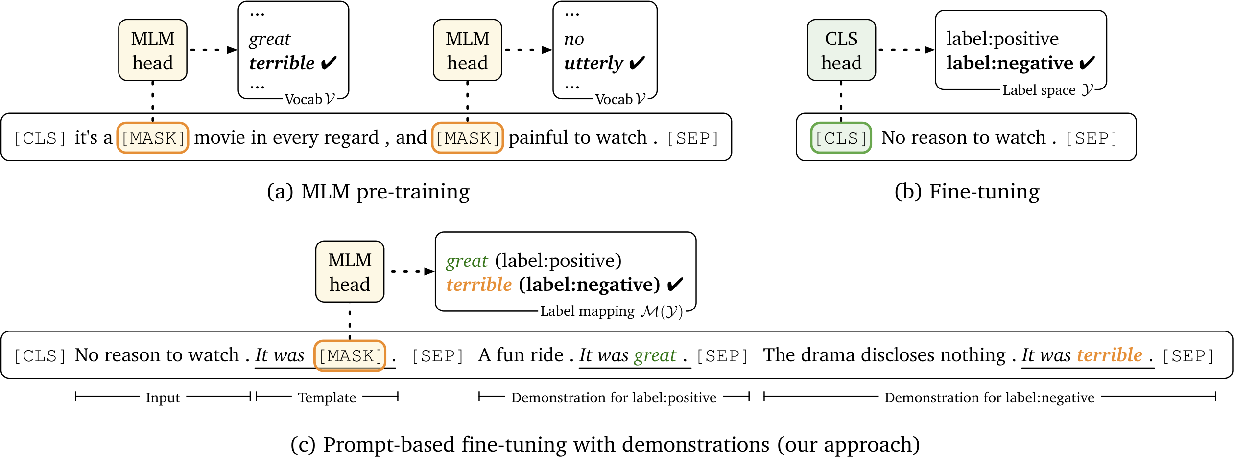
First, we follow the route of prompt-based prediction, first developed by the GPT series [4, 5, 1] for zero-shot prediction and recently studied by PET [6, 7] for fine-tuning. Prompt-based prediction treats the downstream task as a (masked) language modeling problem, where the model directly generates a textual response (referred to as a label word) to a given prompt defined by a task-specific template (see Figure 1(c)). Finding the right prompts, however, is an art—requiring both domain expertise and an understanding of the language model's inner workings. Even if significant effort is invested, manual prompts are likely to be suboptimal. We address this issue by introducing automatic prompt generation, including a pruned brute-force search to identify the best working label words, and a novel decoding objective to automatically generate templates using the generative T5 model [8]—all of which only require the few-shot training data. This allows us to cheaply obtain effective prompts that match or outperform our manually chosen ones.

Second, we adopt the idea of incorporating demonstrations as additional context. GPT-3's naive "in-context learning" paradigm picks up to 32 randomly sampled examples, and concatenates them with the input. This method is not guaranteed to prioritize the most informative demonstrations, and mixing random examples from different classes together creates long contexts which can be hard to learn from. Additionally, the number of usable demonstrations is bounded by the model's maximum input length. We develop a more refined strategy, where, for each input, we randomly sample a single example at a time from each class to create multiple, minimal demonstration sets. We also devise a novel sampling strategy that pairs inputs with similar examples, thereby providing the model with more discriminative comparisons.

We present a systematic evaluation for analyzing few-shot performance on 8 single-sentence and 7 sentence-pair NLP tasks. We observe that given a small number of training examples, (1) prompt-based fine-tuning largely outperforms standard fine-tuning; (2) our automatic prompt search method matches or outperforms manual prompts; and (3) incorporating demonstrations is effective for fine-tuning, and boosts few-shot performance. Together, these simple-yet-effective methods contribute towards a dramatic improvement across the tasks we evaluate on, and we obtain gains up to 30% absolute improvement (11% on average) compared to standard fine-tuning. For instance, we find that a RoBERTa-large model achieves around 90% accuracy on most binary sentence classification tasks, while only relying on 32 training examples. We refer to our approach as LM-BFF, better few-shot fine-tuning of language models: a strong, task-agnostic method for few-shot learning.

2. Related Work

Section Summary: This section reviews prior research on prompting techniques for language models, including work inspired by GPT and PET that uses limited labeled examples to guide predictions, as well as methods for automatically discovering effective prompts rather than relying on manual design. It also covers studies on stabilizing the fine-tuning process for these models and broader few-shot learning approaches such as semi-supervised or meta-learning methods. The authors distinguish their focus by emphasizing minimal assumptions, relying only on a handful of examples and a pre-trained model to advance prompt-based fine-tuning in extreme low-data settings.

Language model prompting. The GPT series ([4, 5, 1]) fueled the development of prompt-based learning, and we follow many of its core concepts. We are also greatly inspired by the recent PET work ([6, 7]), although they mainly focus on a semi-supervised setting where a large set of unlabeled examples are provided. We only use a few annotated examples as supervision, and also explore automatically generated prompts and fine-tuning with demonstrations. Furthermore, we deviate from their evaluation by providing a more rigorous framework, as we will discuss in § 3. Finally, there is a large body of work on prompting for mining knowledge from pre-trained models [9, 10, 11, 12]. Different from these works, we focus on leveraging prompting for fine-tuning on downstream tasks.

Automatic prompt search.

[6] and [13] explore ways of identifying label words automatically, however, none of these results lead to better performance compared to hand-picked ones. In contrast, our method searches over both templates and label words, and is able to match or outperform our manual prompts. Several other attempts have been made in addition—yet these approaches either operate in limited domains, such as finding patterns to express specific relations [14], or require a large number of examples for gradient-guided search [15, 16]. Our approach aims to develop general-purpose search methods that rely only on a few annotations.

Fine-tuning of language models.

A number of recent studies have focused on better methods for fine-tuning language models [17, 18, 19, 20]. These works mainly focus on optimization and regularization techniques to stabilize fine-tuning. Here we use standard optimization techniques, and instead mainly focus our efforts on better prompt-based fine-tuning in a more extreme few-shot setting. We anticipate that results of these studies are largely complementary to ours.

Few-shot learning.

Broadly speaking, our setting is also connected to other few-shot learning paradigms in NLP, including (1) semi-supervised learning [21, 22, 23], where a set of unlabeled examples are given; (2) meta-learning [24, 25, 26, 27, 28], where a set of auxiliary tasks are given; and (3) intermediate training [29, 30], where a related, intermediate task is given. We deviate from these settings by making minimal assumptions about available resources: we only assume a few annotated examples and a pre-trained language model. Our focus is on understanding how far we can push without any other advantages.

::: {caption="Table 1: Manual templates and label words that we used in our experiments. STS-B is a regression task (§ 4.2)."}

:::

3. Problem Setup

Section Summary: In this setup, the goal is to fine-tune a pre-trained language model on a classification task using only a small number of labeled examples—specifically 16 per class, for a total of a few dozen training instances—while relying on an equally small development set for tuning. Experiments cover a range of single-sentence and sentence-pair tasks drawn from GLUE and similar benchmarks, with model development deliberately limited to just two of them to preserve a realistic few-shot scenario on the rest. To handle the high variability that arises from tiny datasets, results are averaged across multiple random splits of the data, with hyper-parameters re-tuned for each split.

Task formulation.

In this work, we assume access to a pre-trained language model $\mathcal{L}$ that we wish to fine-tune on a task $\mathcal{D}$ with a label space $\mathcal{Y}$. For the task, we only assume $K$ training examples per class[^1] for the task's training set $\mathcal{D}{\text{train}}$, such that the total number of examples is $K{\text{tot}} = K \times | \mathcal{Y}|$, and $\mathcal{D}{\text{train}} = {({x}{\mathrm{in}}^i, y^i)}{i=1}^{K{\text{tot}}}$. Our goal is then to develop task-agnostic learning strategies that generalize well to an unseen test set $({x}{\mathrm{in}}^{\text{test}}, y^{\text{test}})\sim \mathcal{D}{\text{test}}$. For model selection and hyper-parameter tuning, we assume a development set $\mathcal{D}{\text{dev}}$, of the same size as the few-shot training set, i.e., $| \mathcal{D}{\text{dev}}| = | \mathcal{D}_{\text{train}}|$. This distinction is important: using a larger development set confers a significant advantage (see our experiments in Appendix A), and subverts our initial goal of learning from limited data.[^2] For all of the following experiments (unless specified otherwise), we take $\mathcal{L}=$ RoBERTa-large and $K=16$.

[^1]: For regression, we partition the data into two "classes" according to being above or below the median value.

[^2]: In contrast, [6, 7] do not use a development set, and adopt a set of hyper-parameters based on practical considerations. This is akin to "shooting in the dark" on a setting that we show can have unintuitive outcomes.

Evaluation datasets.

We conduct a systematic study across $8$ single-sentence and $7$ sentence-pair English tasks, including 8 tasks from the GLUE benchmark [31], SNLI [32], and 6 other popular sentence classification tasks (SST-5, MR, CR, MPQA, Subj, TREC). All of the dataset details are provided in Appendix B. For single-sentence tasks, the goal is to make a prediction based on an input sentence ${x}{\mathrm{in}} = x_1$, such as whether a movie review is positive or not. For sentence-pair tasks, the goal is to take a pair of input sentences ${x}{\mathrm{in}} = (x_1, x_2)$ and predict the relationship between them. We also interchangeably refer to the inputs as <$S_1$> or (<$S_1$>, <$S_2$>). Note that we mainly use SST-2 and SNLI for pilot experiments and model development, making it close to a true few-shot setting, at least for all the other datasets we evaluate on.

Evaluation protocol.

Systematically evaluating few-shot performance can be tricky. It is well-known that fine-tuning on small datasets can suffer from instability [18, 20], and results may change dramatically given a new split of data. To account for this, we measure average performance across 5 different randomly sampled $\mathcal{D}{\text{train}}$ and $\mathcal{D}{\text{dev}}$ splits. This issue has also been discussed in [7]—they suggest using a fixed set of training examples. We argue that sampling multiple splits gives a more robust measure of performance, and a better estimate of the variance. We also observe that hyper-parameters can make a significant difference, thus we sweep multiple hyper-parameters for each data sample, and take the best setting as measured on the $\mathcal{D}_{\text{dev}}$ of that sample (see Appendix C.1).

4. Prompt-based Fine-tuning

Section Summary: Prompt-based fine-tuning reframes classification or regression tasks as masked language modeling problems by wrapping each input in a natural-language template containing a [MASK] token. The model then predicts label words (such as “great” or “terrible”) at the mask position, reusing its already-trained output weights instead of adding a new classification layer on the [CLS] token. This approach narrows the gap between pre-training and fine-tuning, avoids thousands of randomly initialized parameters, and often yields stronger results when only a few dozen labeled examples are available, though performance still depends heavily on the choice of template and label words.

Given a masked language model $\mathcal{L}$, we first convert input ${x}{\mathrm{in}}$ to a token sequence $\tilde{x}$, and the language model $\mathcal{L}$ then maps $\tilde{x}$ to a sequence of hidden vectors ${\mathbf{h}k \in \mathbb{R}^d}$. During standard fine-tuning, we usually take $\tilde{x}{\text{single}} = \texttt{[CLS]} x_1 \texttt{[SEP]}$ or $\tilde{x}{\text{pair}} = \texttt{[CLS]} x_1 \texttt{[SEP]} x_2 \texttt{[SEP]}$. For downstream classification tasks with a label space $\mathcal{Y}$, we train a task-specific head, $\mathrm{softmax}(\mathbf{W}o \mathbf{h}{\texttt{[CLS]}})$, by maximizing the log-probability of the correct label, where $\mathbf{h}_{\texttt{[CLS]}}$ is the hidden vector of [CLS], and $\mathbf{W}_o \in \mathbb{R}^{\mathcal{| \mathcal{Y}|} \times d}$ is a set of randomly initialized parameters introduced at the start of fine-tuning. Similarly, for a regression task, we can introduce $\mathbf{w}_o \in \mathbb{R}^d$ and optimize the mean squared error between $\mathbf{w}o \cdot \mathbf{h}{\texttt{[CLS]}}$ and the gold label. In either case, the number of new parameters can be substantial—for example, a simple binary classification task will introduce 2,048 new parameters for a RoBERTa-large model—making it challenging to learn from a small amount of annotated data (e.g., 32 examples).

An alternative approach to solving this problem is prompt-based fine-tuning, in which $\mathcal{L}$ is directly tasked with "auto-completing" natural language prompts. For instance, we can formulate a binary sentiment classification task using a prompt with input $x_1$ (e.g., "No reason to watch it .") as:

$ x_{\mathrm{prompt}} = \text{\texttt{[CLS]}}x_1\text{{It was}~ \texttt{[MASK]}~. \texttt{[SEP]}} $

and let $\mathcal{L}$ decide whether it is more appropriate to fill in "great" (positive) or "terrible" (negative) for [MASK]. We now formalize this approach for classification and regression (§ 4.1 and § 4.2), and discuss the importance of prompt selection (§ 4.3).

4.1 Classification

Let $\mathcal{M} \colon \mathcal{Y} \rightarrow \mathcal{V}$ be a mapping from the task label space to individual words[^3] in the vocabulary $\mathcal{V}$ of $\mathcal{L}$. Then for each ${x}{\mathrm{in}}$, let the manipulation ${x}{\mathrm{prompt}} = \mathcal{T}({x}_{\mathrm{in}})$ be a masked language modeling (MLM) input which contains one [MASK] token. In this way, we can treat our task as an MLM, and model the probability of predicting class $y \in \mathcal{Y}$ as:

[^3]: More generally, we can consider a one-to-many mapping $\mathcal{M}\colon \mathcal{Y} \rightarrow 2^{| \mathcal{Y}|}$ in which we map labels to sets of words. However, we did not find significant gains in our experiments.

$ \begin{aligned} p(y \mid {x}{\mathrm{in}}) &= p\left(\texttt{[MASK]} = \mathcal{M}(y) \mid x{\mathrm{prompt}}\right) \ &=\frac{\exp\left(\mathbf{w}{\mathcal{M}(y)} \cdot \mathbf{h}{\texttt{[MASK]}}\right)}{\sum_{y' \in \mathcal{Y}} {\exp\left(\mathbf{w}{\mathcal{M}(y')} \cdot \mathbf{h}{\texttt{[MASK]}}\right)}}, \end{aligned} $

where $\mathbf{h}_{\texttt{[MASK]}}$ is the hidden vector of [MASK] and $\mathbf{w}v$ denotes the pre-softmax vector corresponding to $v \in \mathcal{V}$. When supervised examples ${({x}{\mathrm{in}}, y)}$ are available, $\mathcal{L}$ can be fine-tuned to minimize the cross-entropy loss. It is important to note that this approach re-uses the pre-trained weights $\mathbf{w}_v$ and does not introduce any new parameters. It also reduces the gap between pre-training and fine-tuning, making it more effective in few-shot scenarios.

4.2 Regression

We assume the same basic setup as in classification, but treat the label space $\mathcal{Y}$ as a bounded interval $[v_l, v_u]$. Inspired by [33], we model the problem as an interpolation between two opposing poles, ${y_l, y_u}$, with values $v_l$ and $v_u$ respectively. For instance, we can formulate our previous sentiment analysis task as a regression problem in the range $[0, 1]$, where we slide between "terrible" ($v_l = 0$) and "great" ($v_u = 1$). In this way, we can express $y$ as a mixture model:

$ y = v_l \cdot p(y_l \mid {x}{\mathrm{in}}) + v_u \cdot p(y_u \mid {x}{\mathrm{in}}), $

where $p(y_u \mid {x}{\mathrm{in}})$ is the probability of $y_u$, and $p(y_l \mid {x}{\mathrm{in}}) = 1 - p(y_u \mid {x}{\mathrm{in}})$. Then we define $\mathcal{M} \colon {y_l, y_u} \rightarrow \mathcal{V}$, and model $p(y_u \mid {x}{\mathrm{in}})$ the same as Eq. (1).

We fine-tune $\mathcal{L}$ to minimize the KL-divergence between the inferred $p(y_u \mid {x}_{\mathrm{in}})$ and the observed mixture weight, $(y - v_l) / (v_u - v_l)$.

::: {caption="Table 2: The impact of templates and label words on prompt-based fine-tuning ($K=16$)."}

{width=70%}

:::

4.3 Manual prompts: the good and the bad

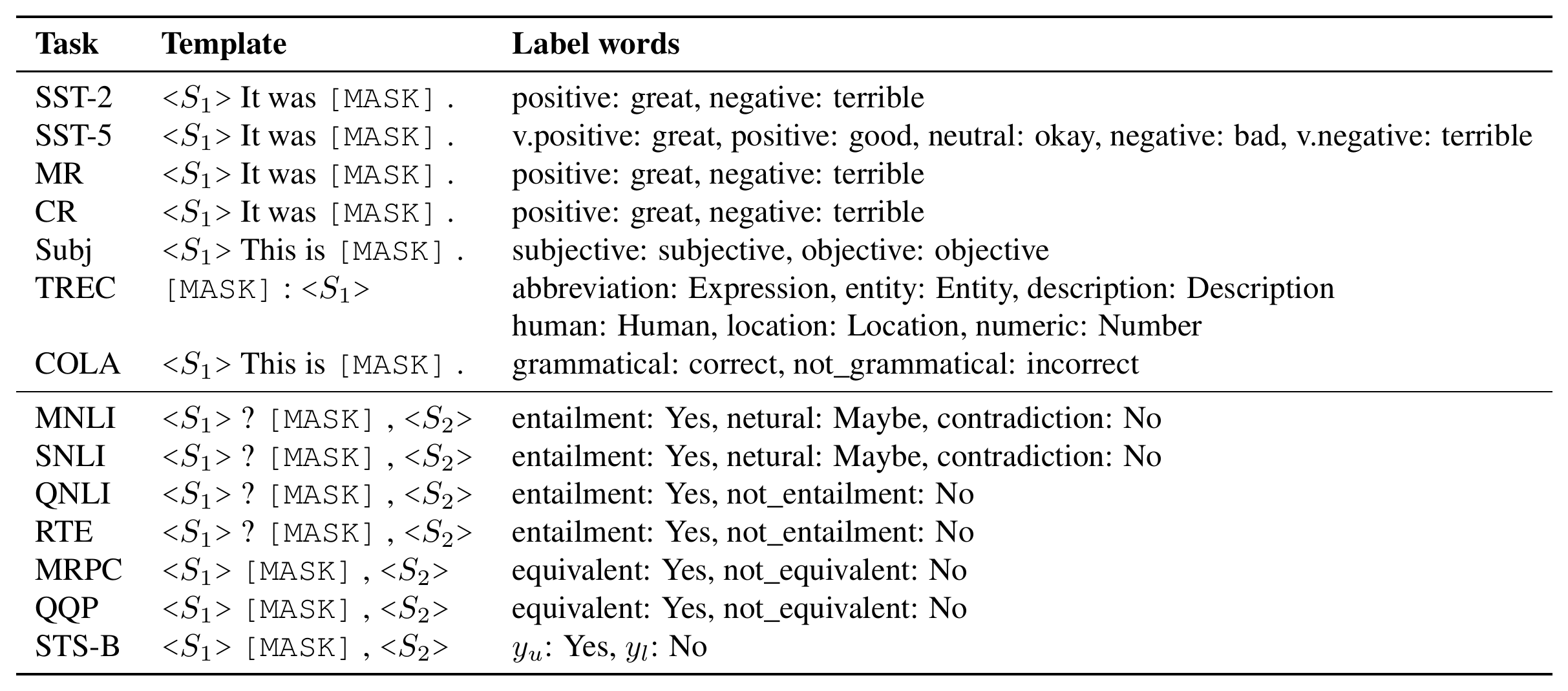
The key challenge is to construct the template $\mathcal{T}$ and label words $\mathcal{M}(\mathcal{Y})$—we refer to these two together as a prompt $\mathcal{P}$. Previous works [6, 7] hand-craft both the templates and label words, which usually requires domain expertise and trial-and-error. Table 1 summarizes manual templates and label words chosen for each dataset in our experiments. These templates and label words were designed by intuition, and by considering formats used in previous literature.

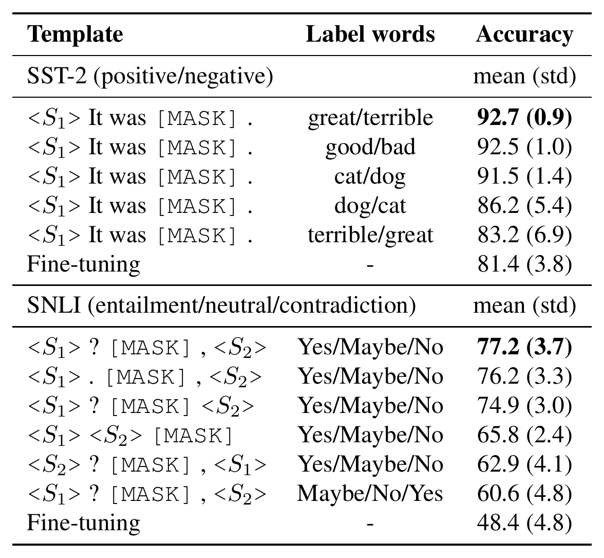
To better understand what constitutes a good template or label word, we conduct a pilot study on SST-2 and SNLI. Table 2 shows that different prompts can lead to substantial differences in final accuracy. Specifically, when a template is fixed, the better the label words match the "semantic classes", the better the final accuracy is (great/terrible

[^4]: It is unclear, however, why RoBERTa thinks that "cat" is more positive than "dog". The authors tend to disagree.

5. Automatic Prompt Generation

Section Summary: The section explores automated methods to reduce manual effort in designing prompts for classification tasks by searching for optimal label words and templates. For label words, it prunes the vocabulary to the most likely candidates per class based on a language model's predictions, then identifies and fine-tunes a small set of promising mappings before selecting the best performer on development data. For templates, it uses a T5 model to generate diverse candidates by filling in placeholders around training examples and label words, followed by beam search decoding, fine-tuning, and selection or ensembling based on development performance.

We now explore principled ways of automating the search process for label words (§ 5.1) and templates (§ 5.2). Our goals are to reduce the human involvement required to design prompts, and to find more optimal settings than those that we manually choose. Here, we assume a classification task, but the process for regression is analogous.

5.1 Automatic selection of label words

We first study how to construct a label word mapping $\mathcal{M}$ that maximizes accuracy on $\mathcal{D}{\text{dev}}$ after fine-tuning, given a fixed template $\mathcal{T}$. Naively searching all possible assignments, however, is (1) generally intractable, as the search space is exponential in the number of classes; and (2) prone to overfitting, as we will tend to uncover spurious correlations given only a few annotations. As a simple solution, for each class $c \in \mathcal{Y}$, we construct a pruned set $\mathcal{V}^c \subset \mathcal{V}$ of the top $k$ vocabulary words based on their conditional likelihood using the initial $\mathcal{L}$. That is, let $\mathcal{D}{\text{train}}^c \subset \mathcal{D}_{\text{train}}$ be the subset of all examples of class $c$. We take $\mathcal{V}^c$ as

$ \displaystyle \underset{v \in \mathcal{V}}{\mathrm{Top}\text{-}k} \left{\sum_{{x}{\mathrm{in}} \in \mathcal{D}{\text{train}}^c} \log P_{\mathcal{L}}\Big(\texttt{[MASK]} = v \mid \mathcal{T}({x}_{\mathrm{in}})\Big)\right}, $

where ${P}{\mathcal{L}}$ denotes the output probability distribution of $\mathcal{L}$. To further narrow down the search space, we find the top $n$ assignments over the pruned space that maximize zero-shot accuracy on $\mathcal{D}{\text{train}}$ (both $n$ and $k$ are hyper-parameters, see Appendix C.2). Then we fine-tune all top $n$ assignments, and re-rank to find the best one using $\mathcal{D}_{\text{dev}}$. This approach is similar to the automatic verbalizer search methods in [6, 13], except that we use a much simpler search process (brute-force) and also apply re-ranking—which we find to be quite helpful.

5.2 Automatic generation of templates

Next, we study how to generate a diverse set of templates ${\mathcal{T}}$ automatically from a fixed set of label words $\mathcal{M}(\mathcal{Y})$. To address this challenging problem, we propose to use T5 [8], a large pre-trained text-to-text Transformer. T5 is pre-trained to fill in missing spans (replaced by T5 mask tokens, e.g., <X> or <Y>) in its input. For example, given the input "Thank you <X> me to your party <Y> week", T5 is trained to generate "<X> for inviting <Y> last <Z>", meaning that "for inviting" is the replacement for <X> and "last" is the replacement for <Y>. This is well suited for prompt generation: we can simply take input sentences from $\mathcal{D}_{\text{train}}$ and let the T5 model construct the template $\mathcal{T}$, without having to specify a pre-defined number of tokens for it.

Given an input example $({x}{\mathrm{in}}, y) \in \mathcal{D}{\text{train}}$, we consider the following simple conversions, denoted as $\mathcal{T}{\mathrm{g}}({x}{\mathrm{in}}, y)$, for formulating the T5 model inputs:[^5]

[^5]: We consider putting the label word both before and after the input sentence for single-sentence tasks. However, we find that it is always better to put the label words in the middle (between the two sentences) for sentence-pair tasks.

$ \begin{aligned}\texttt{<}S_1\texttt{>} &\longrightarrow~ \texttt{\textless{}X\textgreater{}}~ \mathcal{M}(y)~ \texttt{\textless{}Y\textgreater{}}~ \texttt{<}S_1\texttt{>},\\texttt{<}S_1\texttt{>} &\longrightarrow~ \texttt{<}S_1\texttt{>}~ \texttt{\textless{}X\textgreater{}}~ \mathcal{M}(y)~ \texttt{\textless{}Y\textgreater{}},\\texttt{<}S_1\texttt{>}, \texttt{<}S_2\texttt{>} &\longrightarrow \texttt{<}S_1\texttt{>}~ \texttt{\textless{}X\textgreater{}}~ \mathcal{M}(y)~ \texttt{\textless{}Y\textgreater{}}~ \texttt{<}S_2\texttt{>}.\end{aligned} $

As shown in Figure 2, we rely on the T5 model to fill in the placeholders. When decoding, our goal here is to find an output that can work well for all examples in $\mathcal{D}{\text{train}}$, i.e., the output template $\mathcal{T}$ that maximizes $\sum{({x}{\mathrm{in}}, y) \in \mathcal{D}{\text{train}}}{\log P_{\text{T5}}(\mathcal{T} \mid \mathcal{T}{\mathrm{g}}({x}{\mathrm{in}}, y))}$, where $P_{\text{T5}}$ denotes the output probability distribution of T5. It can be decomposed according to:

$ \displaystyle \sum_{j = 1}^{| \mathcal{T}|}\sum_{\quad ; ({x}{\mathrm{in}}, y) \in \mathcal{D}{\text{train}}} {\log{P_{\text{T5}}\big(t_j \mid t_1,...,t_{j-1}, \mathcal{T}{\mathrm{g}}\big({x}{\mathrm{in}},y\big)\big)}}, $

where $(t_1, \ldots, t_{| \mathcal{T}|})$ are the template tokens.

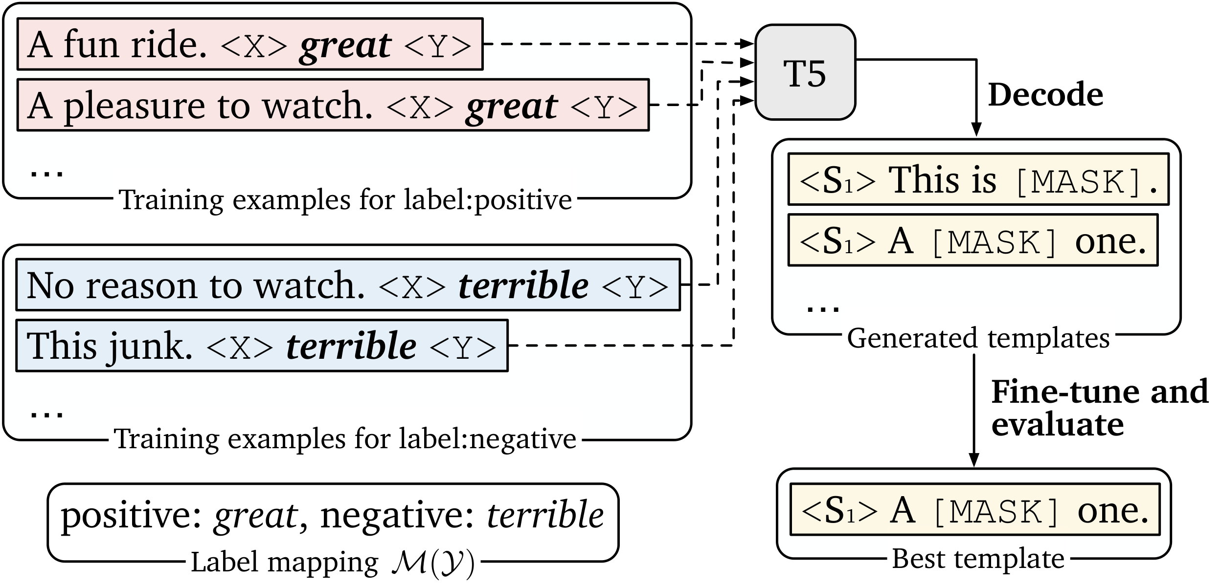
We use beam search to decode multiple template candidates. Concretely, we use a wide beam width (e.g., 100) to cheaply obtain a large set of diverse templates. We then fine-tune each generated template on $\mathcal{D}{\text{train}}$ and use $\mathcal{D}{\text{dev}}$ to either pick the single template with the best performance (Table 3), or the top $k$ templates to use as an ensemble (Table 4). Though it might appear to be expensive to fine-tune the model on each individual template, this is fast in practice due to the small size of $\mathcal{D}_{\text{train}}$, and is also fully automated: making it easy to use, compared to manually tuning prompts for each dataset.

6. Fine-tuning with Demonstrations

Section Summary: In this section the authors explore how to incorporate training examples as demonstrations when fine-tuning medium-sized language models, rather than relying on GPT-3-style in-context learning. Their approach samples one labeled example per class at each step, formats these examples with the task template, and concatenates them with the current input during both training and inference, allowing the model to see multiple such sets through ensembling. They further improve results by restricting the sampled demonstrations to those that are semantically closest to the input query, measured via sentence embeddings from a pretrained model.

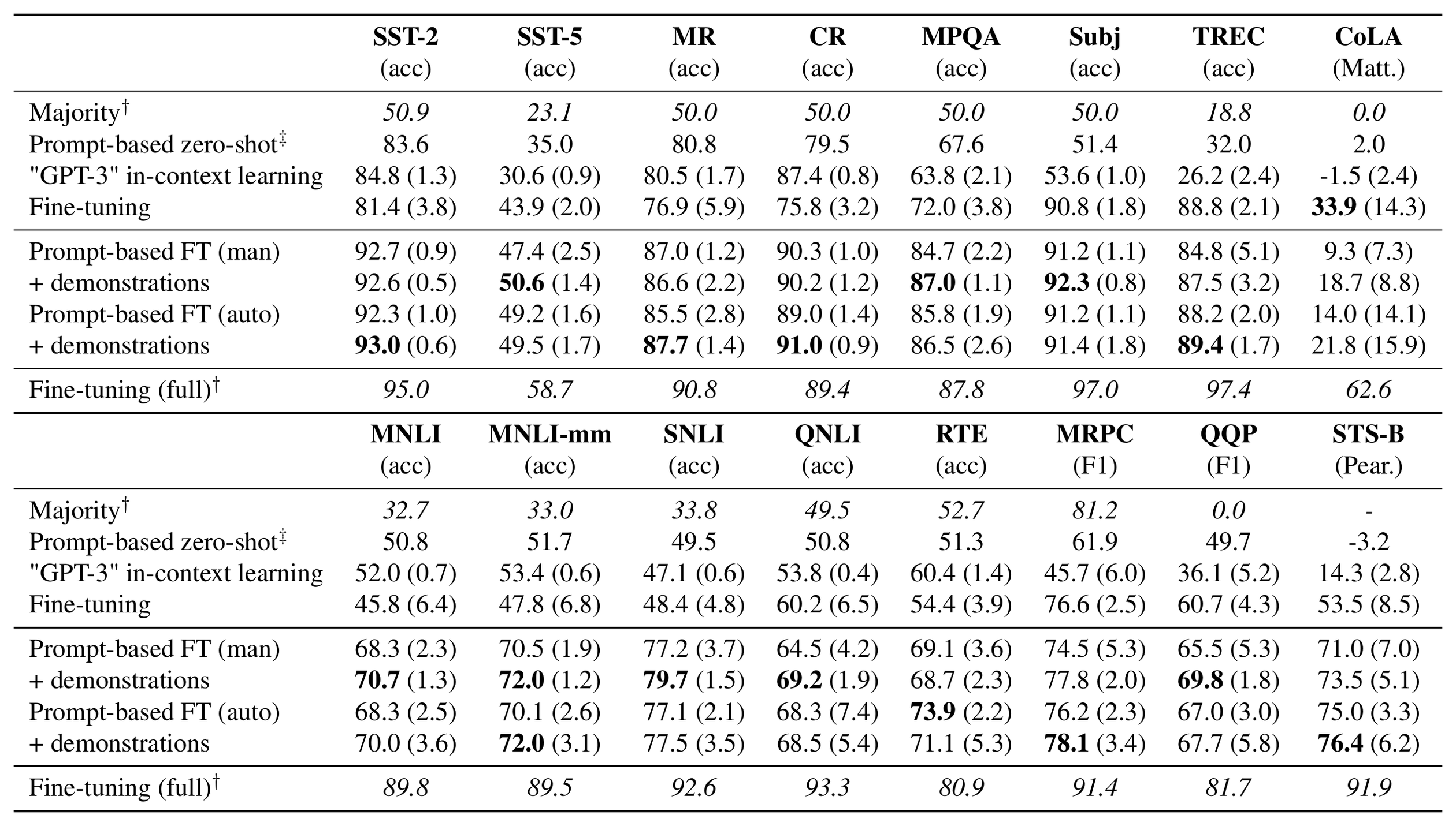
::: {caption="Table 3: Our main results using RoBERTa-large. $†$: full training set is used (see dataset sizes in Table 9); $‡$: no training examples are used; otherwise we use $K = 16$ (per class) for few-shot experiments. We report mean (and standard deviation) performance over 5 different splits (§ 3). Majority: majority class; FT: fine-tuning; man: manual prompt (Table 1); auto: automatically searched templates (§ 5.2); 'GPT-3' in-context learning: using the in-context learning proposed in [1] with RoBERTa-large (no parameter updates)."}

:::

In this section, we study whether we can leverage demonstrations when fine-tuning medium-sized LMs, and find better ways to exploit them.

6.1 Training examples as demonstrations

GPT-3's naive approach to in-context learning simply involves concatenating the input with up to 32 examples randomly drawn from the training set. This approach is suboptimal as (1) the number of available demonstrations is bounded by the model's maximum input length;[^6] and (2) mixing numerous random examples from different classes together creates extremely long contexts which can be hard to leverage, especially for a smaller model. To address these issues, we propose a simpler solution: at each training step, we randomly sample one[^7] example $\big({x}{\mathrm{in}}^{(c)}, y{\phantom{t}}^{(c)}\big)\in \mathcal{D}{\text{train}}$ from each class, convert it into $\mathcal{T}\big({x}{\mathrm{in}}^{(c)}\big)$ with [MASK] replaced by $\mathcal{M}(y_{\phantom{t}}^{(c)})$—we denote this as $\tilde{\mathcal{T}}\big({x}{\mathrm{in}}^{(c)}, y{\phantom{t}}^{(c)}\big)$—and then concatenate them with ${x}_{\mathrm{in}}$ (Figure 1(c)):

[^6]: GPT-3 uses a context size of 2,048 while most smaller language models (e.g., RoBERTa) have a context size of 512.

[^7]: We also explored sampling multiple examples per class, but did not observe any improvements.

$ \displaystyle \mathcal{T}\big({x}{\mathrm{in}}\big) \oplus \tilde{\mathcal{T}}\big({x}{\mathrm{in}}^{(1)}, y_{\phantom{t}}^{(1)}\big) \oplus \cdots \oplus \tilde{\mathcal{T}}\big({x}{\mathrm{in}}^{(| \mathcal{Y}|)}, y{\phantom{t}}^{(| \mathcal{Y}|)}\big). $

Here $\oplus$ denotes concatenation of input sequences. During both training and inference we sample multiple demonstration sets for each ${x}{\mathrm{in}}$. Note that both ${x}{\mathrm{in}}$ and demonstration examples are sampled from the same set $\mathcal{D}{\text{train}}$ during training. At testing time, we still sample demonstration sets from $\mathcal{D}{\text{train}}$ and ensemble predictions across all sets.

6.2 Sampling similar demonstrations

We observe that controlling the construction of the demonstration examples ${({x}{\mathrm{in}}^{(c)}, y{\phantom{t}}^{(c)})}$ is crucial for good final performance. For example, if the set of contrastive demonstrations ${x}{\mathrm{in}}^{(c)}$ are all dramatically different—from each other, or from the query ${x}{\mathrm{in}}$—then it becomes challenging for the language model to decipher meaningful patterns. As a result, the model may simply ignore the context, or even get confused by the additional examples. To address this issue, we devise a simple strategy in which we only sample examples that are semantically close to ${x}{\mathrm{in}}$. Specifically, we use a pre-trained SBERT [34] model to obtain embeddings for all input sentences (for sentence-pair tasks, we use the concatenation of the two sentences). Here we just feed the raw sentences without the templates into SBERT. For each query ${x}{\mathrm{in}}$ and each label $c\in \mathcal{Y}$, we sort all training instances with the label $x \in \mathcal{D}{\text{train}}^{c}$ by their similarity score to the query $\cos(\mathbf{e}({x}{\mathrm{in}}), \mathbf{e}(x))$, and only sample from the top $r = 50%$ instances for each class to use as demonstrations.

7. Experiments

Section Summary: The experiments evaluate the LM-BFF method on RoBERTa-large using only 16 training examples per class across several classification tasks. Prompt-based fine-tuning with either manually designed or automatically generated prompts substantially outperforms standard fine-tuning, and adding in-context demonstrations yields further gains that reach 30% on SNLI and 11% on average. Automatic template search produces prompts that match or exceed manual ones, ensembles of multiple such prompts improve results over single models, and selective sampling of demonstrations consistently beats random selection.

We present our main results, and address several research questions pertaining to our LM-BFF approach. Implementation details are in Appendix C.

7.1 Main results

We use a RoBERTa-large model and set $K = 16$ in our experiments. A comparison of using RoBERTa vs BERT can be found in Appendix D. For automatic prompt search, in our main table we report automatic template search only (which consistently performs the best, see Table 5). To put our results in perspective, we compare to a number of baselines, namely (1) standard fine-tuning in our few-shot setting; (2) standard fine-tuning using the full training set; (3) simply taking the most frequent class (measured on the full training set); (4) prompt-based zero-shot prediction where we take our manual prompts and use $\mathcal{L}$ "out-of-the-box" without using any training examples; and (5) "GPT-3" in-context learning, where we use the same prompt-based zero-shot setting, but augment the context with randomly sampled 32 demonstrations (and still use RoBERTa-large, not GPT-3).

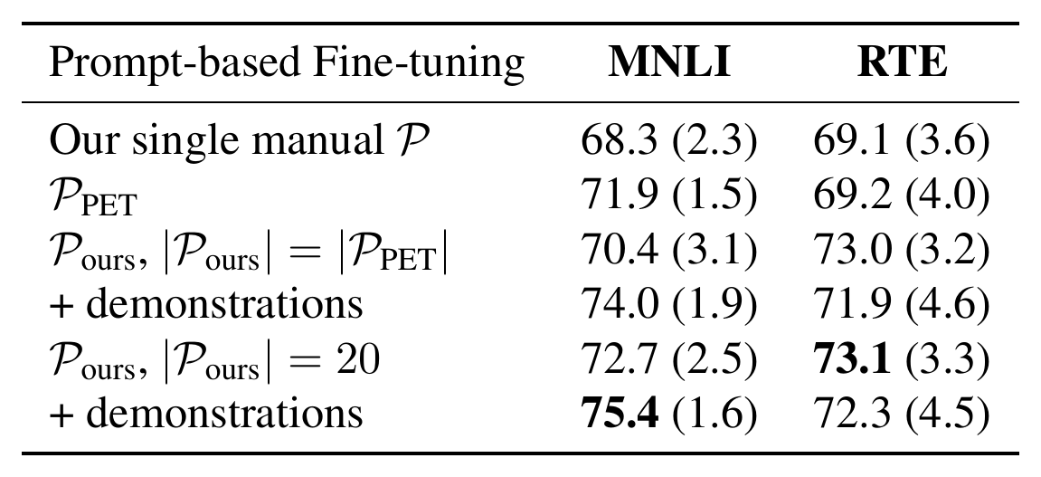
::: {caption="Table 4: Ensemble models using manual prompts from PET [6, 7] and our automatic templates. PET uses 4 prompts for MNLI and 5 for RTE. We also use an equal number of templates in $|\mathcal{P}{\text{ours}}| = |\mathcal{P}{\text{PET}}|$ for a fair comparison."}

{width=70%}

:::

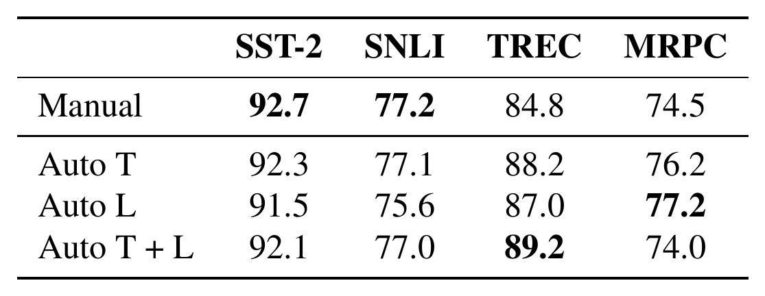
::: {caption="Table 5: Comparison between manual prompts and different automatic prompt generation methods: auto-generated templates (Auto T), auto-generated label words (Auto L), and their combination (Auto T + L)."}

{width=70%}

:::

Single-prompt results.

Table 3 shows our main results using a single prompt, either from our manually designed ones (Table 1), or the best generated ones. First, prompt-based zero-shot prediction achieves much better performance than the majority class, showing the pre-encoded knowledge in RoBERTa. Also, "GPT-3" in-context learning does not always improve over zero-shot prediction, likely because smaller language models are not expressive enough to use off-the-shelf like GPT-3.

Second, prompt-based fine-tuning can greatly outperform standard fine-tuning, both when using a manual prompt or a generated one. CoLA is one interesting exception, as the input may be a non-grammatical sentence which is out of the distribution of $\mathcal{L}$. Generally, our automatically searched templates can achieve comparable or even higher results than manual ones, especially for tasks in which constructing strong manual templates is less intuitive (e.g., TREC, QNLI and MRPC).

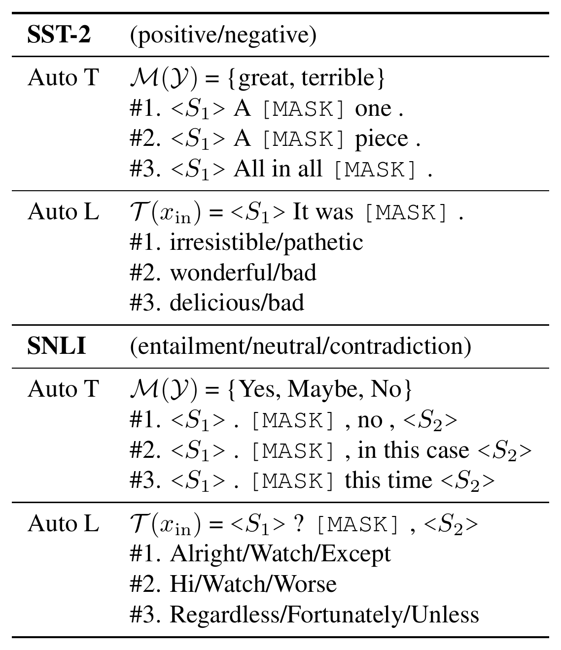
::: {caption="Table 6: Examples of our automatically generated templates (Auto T) and label words (Auto L)."}

{width=70%}

:::

Finally, using demonstrations in context leads to consistent gains in a majority of tasks. In summary, our combined solution—fine-tuning with automatically searched templates and sampled demonstration sets—achieves a $30%$ gain on SNLI compared to standard fine-tuning, and $11%$ gain on average.

Ensemble results.

An advantage of automatic prompt search is that we can generate as many prompts as we want, train individual models, and create large ensembles. PET [6, 7] also ensembles multiple models trained with manual prompts.[^8] In Table 4, we make a direct comparison of our searched prompts and PET's manual prompts on MNLI and RTE (two datasets that we evaluate in common).[^9] As the results show, an ensemble with multiple templates always improves performance. An ensemble of the same number of automatic templates achieves comparable or better performance than the ensemble of PET's manual prompts. Increasing the number of automatic templates brings further gains.

[^8]: They then use unlabeled data and distillation to get a single model, which is outside of our scope.

[^9]: In the PET NLI templates, the hypothesis is put before the premise, which we actually found to be suboptimal. In our experiments, we swap the two and get better results.

7.2 Analysis of generated prompts

Table 5 gives the results of using manual vs automatic prompts. For automatic prompts, we compare template search (Auto T), label word search (Auto L), and a joint variant (Auto T + L) in which we start from manual label words, apply Auto T, and then Auto L. In most cases, Auto T achieves comparable or higher performance than manual ones, and is consistently the best variant. Auto L outperforms manual prompts on TREC and MRPC—but is considerably worse on SNLI. Auto T + L is often better than Auto L, but only sometimes better than Auto T. Table 6 shows examples from Auto T and Auto L (A full list in Appendix E). Auto T templates generally fit the context and label words well, but can contain biased peculiarities (e.g., "Yes/No, no" in SNLI). For Auto L words, things are mixed: while most look intuitively reasonable, there are also some mysterious abnormalities (e.g., "Hi" for the "entailment" class in SNLI).

7.3 Analysis of demonstration sampling

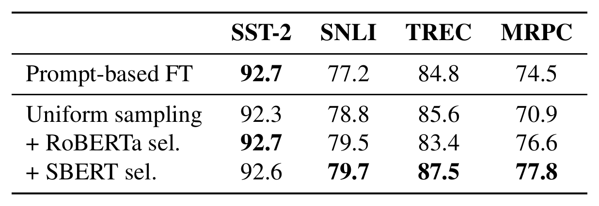
::: {caption="Table 7: Impact of demonstration sampling strategies. Uniform sampling randomly samples demonstrations, while selective (sel.) sampling only takes top sentences measured by the sentence encoders (§ 6)."}

{width=70%}

:::

Table 7 compares the performance of demonstrations using uniform sampling to selective sampling by SBERT. We acknowledge that SBERT is trained on SNLI and MNLI datasets, thus we also tried a simple sentence encoder using mean pooling of hidden representations from RoBERTa-large. We find that in either case, using selective sampling outperforms uniform sampling, highlighting the importance of sampling similar examples for incorporating demonstrations in context.

7.4 Sample efficiency

Figure 3 illustrates how standard fine-tuning and our LM-BFF compare as $K$ increases. For a simple task such as SST-2 (also see MR, CR and MPQA in Table 3), despite using only 32 total examples, LM-BFF has already nearly saturated its performance and is comparable to standard fine-tuning over the entire dataset. On the harder task of SNLI, LM-BFF continues to improve as $K$ increases while still maintaining a performance gap over standard fine-tuning, until the two converge around $K = 256$.

8. Discussion

Section Summary: The approach of recasting language tasks as fill-in-the-blank problems improves results when only a handful of examples are available, yet it still trails far behind standard training on thousands of examples and produces highly variable outcomes. Automatic prompt creation works reasonably well but depends on some human-designed starting points, making it difficult to explore a wider range of options or generalize reliably from roughly 32 examples. The method also works best for simple tasks that naturally fit a short completion format with few possible answers, while more complex problems such as structured prediction remain harder to handle.

Reformulating NLP tasks as MLM has exciting implications for few-shot learning, but also has limitations. First, while LM-BFF greatly outperforms standard fine-tuning, Table 3 shows that, overall, the performance still substantially lags behind fine-tuning with thousands of examples, especially for harder tasks. Additionally, just like standard fine-tuning, our results also suffer from high variance. As described in § 2, several recent studies have tried to counter instability in few-shot fine-tuning and we expect these methods to also help here.

With respect to automatic prompt generation, despite its effectiveness, we still find it practically challenging to expand the search space, or generalize well based on only approximately 32 examples. This is partly due to our lingering reliance on some manual design—either manual templates (for label word search) or manual label words (for template search), which allows us to get our search off the ground, but does also bias it towards areas of the search space that we might have already imagined.

Finally, it is important to clarify that LM-BFF favors certain tasks which (1) can be naturally posed as a "fill-in-the-blank" problem; (2) have relatively short input sequences; and (3) do not contain many output classes. Issues (2) and (3) might be ameliorated with longer-context language models [e.g., 35]. For tasks that are not straightforward to formulate in prompting, such as structured prediction, issue (1) is more fundamental. We leave it as an open question for future work.

:::: {.figure cols="2"}

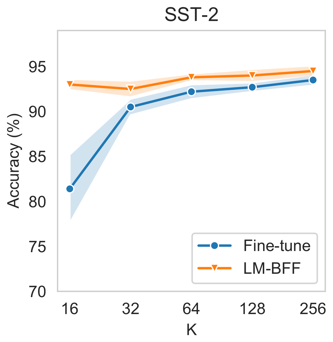
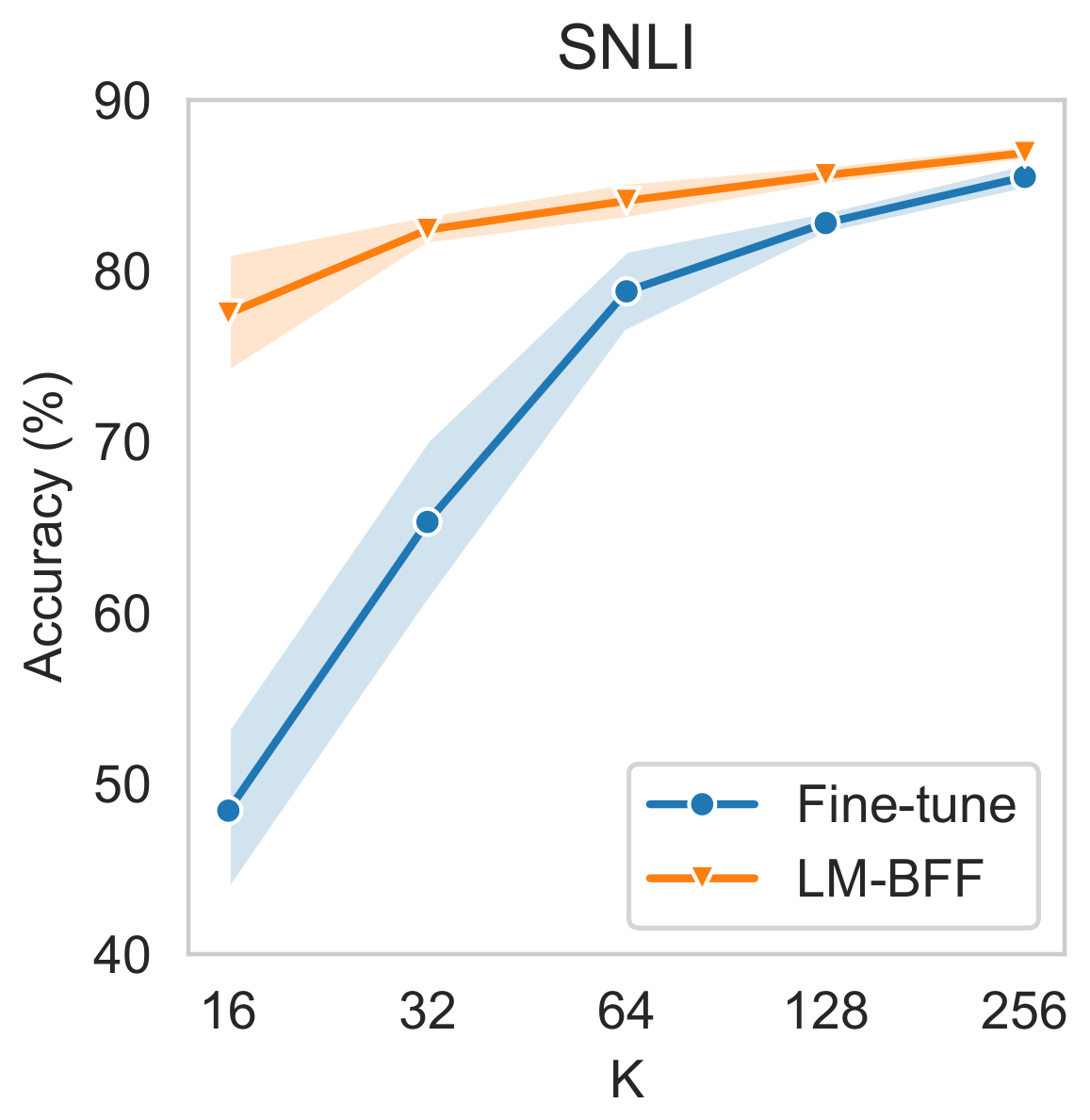
Figure 3: Standard fine-tuning vs our LM-BFF as a function of $K$ (# instances per class). For lower $K$, our method consistently outperforms standard fine-tuning. ::::

9. Conclusion

Section Summary: The paper introduces LM-BFF, a straightforward set of techniques for improving how language models learn from just a few examples. The method relies on automatically found prompts along with selected training examples placed directly in the input, which together produce much stronger results than standard fine-tuning. The authors also note the approach's current limits and outline open questions for future work.

In this paper we presented LM-BFF, a set of simple but effective techniques for fine-tuning language models using only a few examples. Our approach proposes to (1) use prompt-based fine-tuning with automatically searched prompts; and (2) include selected task demonstrations (training examples) as part of the input context. We show that our method outperforms vanilla fine-tuning by up to $30%$ (and $11$% on average). We concluded by discussing the limitations of our approach, and posed open questions for future study.

Acknowledgements

Section Summary: The authors thank colleagues from NLP research groups at Princeton, MIT, and Tsinghua, as well as anonymous reviewers, for their helpful comments on the work. Two of the researchers received personal support through graduate fellowships, one from Princeton University and the other from the National Science Foundation. The project also received partial funding from a Google Research Scholar Award.

We thank the members of Princeton, MIT, Tsinghua NLP groups and the anonymous reviewers for their valuable feedback. TG is supported by a Graduate Fellowship at Princeton University and AF is supported by an NSF Graduate Research Fellowship. This research is also partly supported by a Google Research Scholar Award.

Appendix

Section Summary: The appendix examines how varying development set sizes influence few-shot model performance, noting that larger sets yield better results and justifying the authors' choice to match training and development set sizes. It then describes the specific datasets used from GLUE, SNLI, and other sources, along with how test sets were constructed or sampled for evaluation. Finally, it details the hyper-parameter search process, implementation choices for prompt-based fine-tuning and demonstrations, and a comparison of BERT versus RoBERTa handling of input segments.

o̧unterwithin{figure}{section} o̧unterwithin{table}{section}

A. Impact of Development Sets

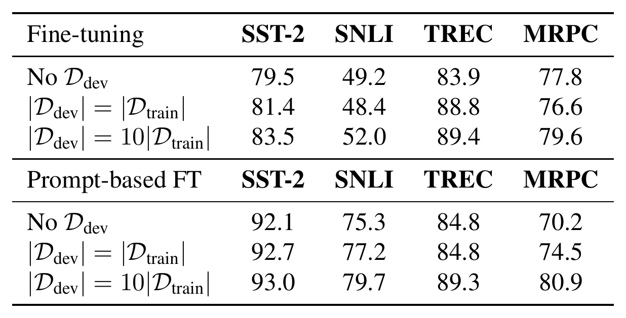
Table 8 shows how the size of the development sets can affect the final performance of the model. For "No $\mathcal{D}{\text{dev}}

::: {caption="Table 8: Impact of different sizes of development sets. Standard deviations are omitted here to save space. For No $| \mathcal{D}_{\text{dev}}|$, we use the same set of hyper-parameters as [6, 7]."}

{width=70%}

:::

B. Datasets

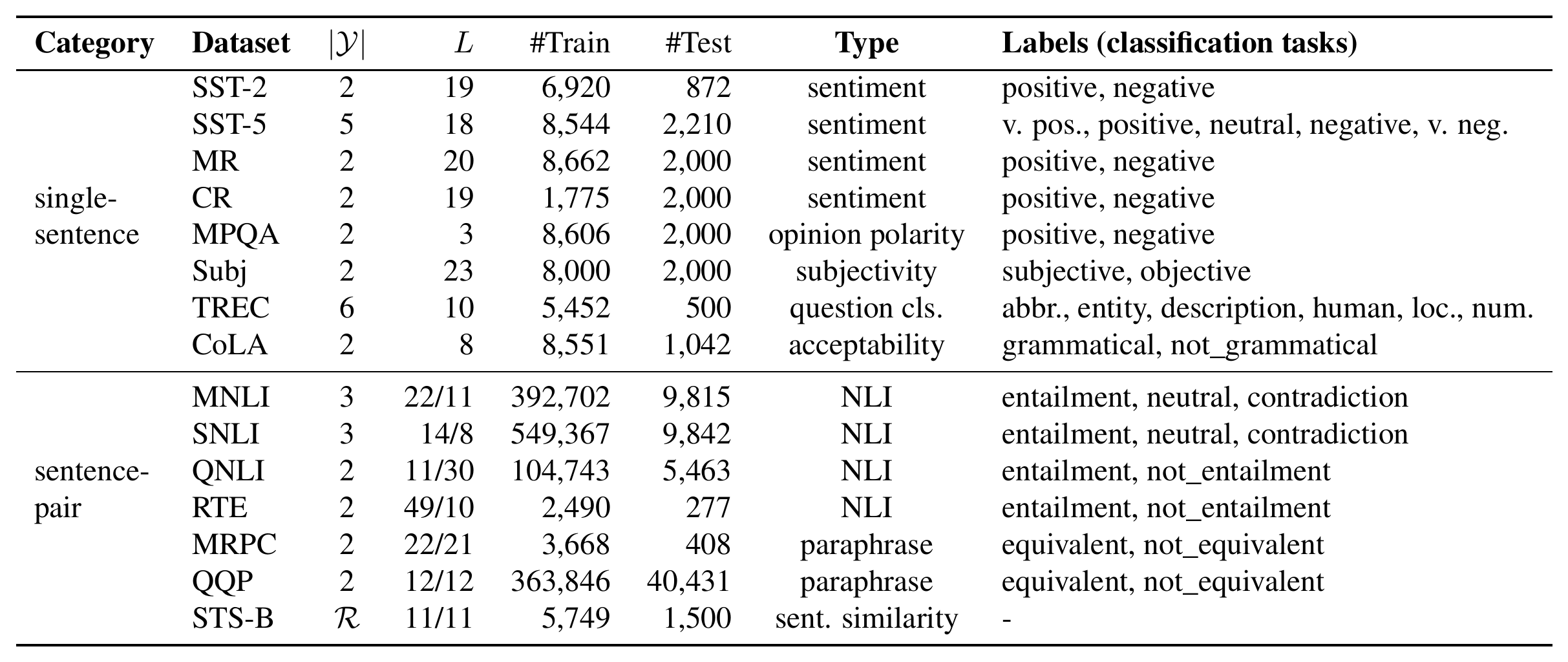
For SNLI [32] and datasets from GLUE [31], including SST-2 [36], CoLA [37], MNLI [38], QNLI [39], RTE [40, 41, 42, 43], MRPC [44], QQP^10 and STS-B [45], we follow [20] and use their original development sets for testing. For datasets which require a cross-validation evaluation—MR [46], CR [47], MPQA [48], Subj [49]—we simply randomly sample 2,000 examples as the testing set and leave them out from training. For SST-5 [36] and TREC [50], we use their official test sets. We show dataset statistics in Table 9.

::: {caption="Table 9: The datasets evaluated in this work. $|\mathcal{Y}|$: # of classes for classification tasks (with one exception: STS-B is a real-valued regression task over the interval $[0, 5]$). $L$: average # of words in input sentence(s). Note that we only sample $\mathcal{D}{\text{train}}$ and $\mathcal{D}{\text{dev}}$ of $K \times | \mathcal{Y}|$ examples from the original training set in our few-shot experiments (§ 3)."}

:::

C. Experimental Details

C.1 Hyper-parameter selection

For grid search, we take learning rates from {1e-5, 2e-5, 5e-5} and batch sizes from 2, 4, 8. These numbers are picked by pilot experiments on the SST-2 and SNLI datasets. We also use early stopping to avoid overfitting. For each trial, we train the model for 1,000 steps, validate the performance every 100 steps, and take the best checkpoint.

C.2 Prompt-based fine-tuning

Table 1 shows all the manual templates and label words we use in experiment. For automatically template generation, we take the T5-3B[^11] model, which is the largest publicly available one that can fit on a single GPU. For automatically searching label words, we set $k$ to 100 for all tasks except SST-5 and TREC. For SST-5 we set a smaller $k = 30$, as it is a 5-way classification task. For TREC, we observe that filtering $\mathcal{V}^c$ using conditional likelihood alone is still noisy, thus we set $k = 1000$, and then re-rank $\mathcal{V}^c$ by the nearest neighbors of the original manual label words and take the top 30 per class. We set $n$ to 100 in all experiments. Due to the large number of trials in automatic search, we take a fixed set of hyper-parameters in this part: batch size of 8 and learning rate of 1e-5.

[^11]: We take the T5 1.0 checkpoint, which is trained on both unsupervised and downstream task data. We compared it to T5 1.1 (without downstream task data) and did not find a significant difference in generated templates.

Since the idea of prompt-based fine-tuning is to make the input and output distribution close to the pre-training, the implementation details are crucial. For templates, we put extra space before sentences if it is not at the beginning of the input. Also, we lowercase the first letter of the sentence if it is concatenated with a prefix (e.g., <$S_2$> in Table 1). Also if one sentence is appended any punctuation (e.g., <$S_1$> in Table 1), then the last character of the original sentence is discarded. Finally, we prepend a space for label words in $\mathcal{M}(\mathcal{Y})$. For example, we use "great" instead of "great" in the RoBERTa vocabulary, where "" stands for space.

C.3 Fine-tuning with demonstrations

When using demonstrations, we sample $16$ different sets of demonstrations for each input and average the predicted log probability for each class during inference. We find that further increasing the number of samples does not bring substantial improvement. Additional, we have tried different aggregation methods like taking the result with the maximum confidence and we did not find a meaningful improvement. For selective demonstrations, we take roberta-large-nli-stsb- mean-tokens^12 from [34] as our sentence embedding model.

D. Comparisons of BERT vs RoBERTa

::: {caption="Table 10: A comparison of BERT-large vs RoBERTa-large. We use manual prompts in these experiments."}

{width=70%}

:::

Table 10 compares the results of BERT-large (uncased) and RoBERTa-large in our settings. Pre-trained BERT provides two segment embeddings (A/B) for different parts of input. The common practice, when fine-tuning BERT, is that using only segment A for single-sentence tasks, and using segment A/B for the two sentences in sentence-pair tasks. In our case of incorporating demonstrations, however, we have more than two sentences. Thus we explore the following different strategies for segments: (1) using the A segment for all sentences (1-seg); (2) using the A segment for the original input and the B segment for the demonstrations (2-seg); (3) using different segment embeddings for each sentence ($n$-seg), e.g., for SNLI, we use different segments for each premise and hypothesis in both the original input and the demonstrations, which leads to a total number of 8 segment embeddings. This introduces new segment embeddings (randomly initialized and learned during fine-tuning) as the pre-trained BERT only has two.

Table 10 shows that prompt-based fine-tuning with demonstrations also works for BERT, and 2-seg works the best when incorporating demonstrations. Still, we take RoBERTa-large as our main model, for RoBERTa performs much better than BERT and RoBERTa saves the trouble to tune the usage of segment embeddings.

E. Generated Prompts

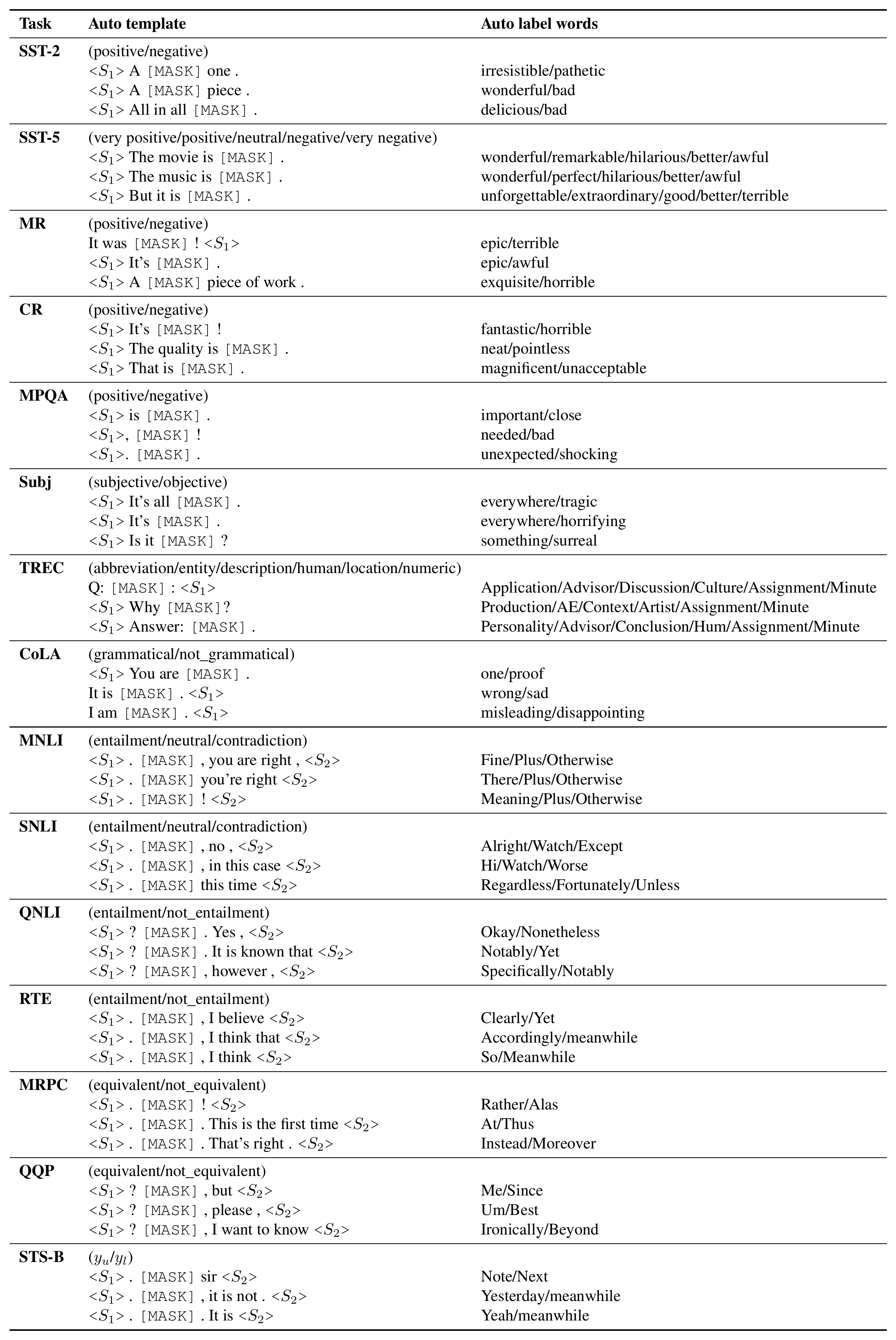
We demonstrate the top 3 automatically generated templates and label words for all tasks in Table 11. In general, most automatic templates are reasonable and grammatically correct. For the label words, the generated results look intuitive for most single sentence tasks. For other tasks, the automatic ones can be counterintuitive in some cases. It is still unclear why the language model picks these words and sometimes they actually work well. We leave this for future study.

::: {caption="Table 11: Top 3 automatically generated templates and label words for all tasks based on one split of $K=16$ training examples. Note that automatic template results are based on manual label words and automatic label word results are based on manual templates provided in Table 1."}

:::

References

Section Summary: This section compiles a bibliography of academic papers and technical reports focused on advances in natural language processing. The cited works examine large language models such as BERT and GPT variants, along with approaches for few-shot learning, prompt engineering, knowledge extraction, and efficient fine-tuning on limited data. Most entries reference publications from major venues like NeurIPS, ACL, EMNLP, and NAACL between 2017 and 2021.

[1] Tom B Brown, Benjamin Mann, Nick Ryder, Melanie Subbiah, Jared Kaplan, Prafulla Dhariwal, Arvind Neelakantan, Pranav Shyam, Girish Sastry, Amanda Askell, et al. 2020. Language models are few-shot learners. In Advances in Neural Information Processing Systems (NeurIPS).

[2] Jacob Devlin, Ming-Wei Chang, Kenton Lee, and Kristina Toutanova. 2019. BERT: Pre-training of deep bidirectional Transformers for language understanding. In North American Chapter of the Association for Computational Linguistics (NAACL).

[3] Yinhan Liu, Myle Ott, Naman Goyal, Jingfei Du, Mandar Joshi, Danqi Chen, Omer Levy, Mike Lewis, Luke Zettlemoyer, and Veselin Stoyanov. 2019. RoBERTa: A robustly optimized BERT pretraining approach. arXiv preprint arXiv:1907.11692.

[4] Alec Radford, Karthik Narasimhan, Tim Salimans, and Ilya Sutskever. 2018. Improving language understanding by generative pre-training. Technical report, OpenAI.

[5] Alec Radford, Jeff Wu, Rewon Child, David Luan, Dario Amodei, and Ilya Sutskever. 2019. Language models are unsupervised multitask learners. Technical report, OpenAI.

[6] Timo Schick and Hinrich Schütze. 2021a. Exploiting cloze questions for few-shot text classification and natural language inference. In European Chapter of the Association for Computational Linguistics (EACL).

[7] Timo Schick and Hinrich Schütze. 2021b. It's not just size that matters: Small language models are also few-shot learners. In North American Chapter of the Association for Computational Linguistics (NAACL).

[8] Colin Raffel, Noam Shazeer, Adam Roberts, Katherine Lee, Sharan Narang, Michael Matena, Yanqi Zhou, Wei Li, and Peter J Liu. 2020. Exploring the limits of transfer learning with a unified text-to-text Transformer. The Journal of Machine Learning Research (JMLR), 21(140).

[9] Trieu H Trinh and Quoc V Le. 2018. A simple method for commonsense reasoning. arXiv preprint arXiv:1806.02847.

[10] Fabio Petroni, Tim Rocktäschel, Sebastian Riedel, Patrick Lewis, Anton Bakhtin, Yuxiang Wu, and Alexander Miller. 2019. Language models as knowledge bases? In Empirical Methods in Natural Language Processing (EMNLP).

[11] Joe Davison, Joshua Feldman, and Alexander M Rush. 2019. Commonsense knowledge mining from pretrained models. In Empirical Methods in Natural Language Processing (EMNLP).

[12] Bibliography entry for citation key "talmor2020olmpics inter alia" was not supplied with the source.

[13] Timo Schick, Helmut Schmid, and Hinrich Schütze. 2020. Automatically identifying words that can serve as labels for few-shot text classification. In International Conference on Computational Linguistics (COLING).

[14] Zhengbao Jiang, Frank F Xu, Jun Araki, and Graham Neubig. 2020. How can we know what language models know? Transactions of the Association of Computational Linguistics (TACL).

[15] Taylor Shin, Yasaman Razeghi, Robert L. Logan IV, Eric Wallace, and Sameer Singh. 2020. AutoPrompt: Automatic prompt construction for masked language models. In Empirical Methods in Natural Language Processing (EMNLP).

[16] Zexuan Zhong, Dan Friedman, and Danqi Chen. 2021. Factual probing is [MASK]: Learning vs. learning to recall. In North American Association for Computational Linguistics (NAACL).

[17] Jeremy Howard and Sebastian Ruder. 2018. Universal language model fine-tuning for text classification. In Association for Computational Linguistics (ACL).

[18] Jesse Dodge, Gabriel Ilharco, Roy Schwartz, Ali Farhadi, Hannaneh Hajishirzi, and Noah Smith. 2020. Fine-tuning pretrained language models: Weight initializations, data orders, and early stopping. arXiv preprint arXiv:2002.06305.

[19] Cheolhyoung Lee, Kyunghyun Cho, and Wanmo Kang. 2020. Mixout: Effective regularization to finetune large-scale pretrained language models. In International Conference on Learning Representations (ICLR).

[20] Tianyi Zhang, Felix Wu, Arzoo Katiyar, Kilian Q Weinberger, and Yoav Artzi. 2021. Revisiting few-sample BERT fine-tuning. In International Conference on Learning Representations (ICLR).

[21] Takeru Miyato, Andrew M Dai, and Ian Goodfellow. 2017. Adversarial training methods for semi-supervised text classification. In International Conference on Learning Representations (ICLR).

[22] Qizhe Xie, Zihang Dai, Eduard Hovy, Thang Luong, and Quoc Le. 2020. Unsupervised data augmentation for consistency training. Advances in Neural Information Processing Systems (NeurIPS), 33.

[23] Jiaao Chen, Zichao Yang, and Diyi Yang. 2020. MixText: Linguistically-informed interpolation of hidden space for semi-supervised text classification. In Association for Computational Linguistics (ACL).

[24] Mo Yu, Xiaoxiao Guo, Jinfeng Yi, Shiyu Chang, Saloni Potdar, Yu Cheng, Gerald Tesauro, Haoyu Wang, and Bowen Zhou. 2018. Diverse few-shot text classification with multiple metrics. In North American Chapter of the Association for Computational Linguistics (NAACL).

[25] Xu Han, Hao Zhu, Pengfei Yu, Ziyun Wang, Yuan Yao, Zhiyuan Liu, and Maosong Sun. 2018. Fewrel: A large-scale supervised few-shot relation classification dataset with state-of-the-art evaluation. In Empirical Methods in Natural Language Processing (EMNLP).

[26] Trapit Bansal, Rishikesh Jha, and Andrew McCallum. 2020a. Learning to few-shot learn across diverse natural language classification tasks. In International Conference on Computational Linguistics (COLING).

[27] Trapit Bansal, Rishikesh Jha, Tsendsuren Munkhdalai, and Andrew McCallum. 2020b. Self-supervised meta-learning for few-shot natural language classification tasks. In Empirical Methods in Natural Language Processing (EMNLP).

[28] Yujia Bao, Menghua Wu, Shiyu Chang, and Regina Barzilay. 2020. Few-shot text classification with distributional signatures. In International Conference on Learning Representations (ICLR).

[29] Jason Phang, Thibault Févry, and Samuel R Bowman. 2018. Sentence encoders on STILTs: Supplementary training on intermediate labeled-data tasks. arXiv preprint arXiv:1811.01088.

[30] Wenpeng Yin, Nazneen Fatema Rajani, Dragomir Radev, Richard Socher, and Caiming Xiong. 2020. Universal natural language processing with limited annotations: Try few-shot textual entailment as a start. In Empirical Methods in Natural Language Processing (EMNLP).

[31] Alex Wang, Amanpreet Singh, Julian Michael, Felix Hill, Omer Levy, and Samuel R Bowman. 2019. GLUE: A multi-task benchmark and analysis platform for natural language understanding. In International Conference on Learning Representations (ICLR).

[32] Samuel Bowman, Gabor Angeli, Christopher Potts, and Christopher D Manning. 2015. A large annotated corpus for learning natural language inference. In Empirical Methods in Natural Language Processing (EMNLP).

[33] Pascal Mettes, Elise van der Pol, and Cees Snoek. 2019. Hyperspherical prototype networks. In Advances in Neural Information Processing Systems (NeurIPS).

[34] Nils Reimers and Iryna Gurevych. 2019. Sentence-BERT: Sentence embeddings using Siamese BERT-networks. In Empirical Methods in Natural Language Processing and International Joint Conference on Natural Language Processing (EMNLP-IJCNLP).

[35] Iz Beltagy, Matthew E. Peters, and Arman Cohan. 2020. Longformer: The long-document Transformer. arXiv:2004.05150.

[36] Richard Socher, Alex Perelygin, Jean Wu, Jason Chuang, Christopher D. Manning, Andrew Ng, and Christopher Potts. 2013. Recursive deep models for semantic compositionality over a sentiment treebank. In Empirical Methods in Natural Language Processing (EMNLP).

[37] Alex Warstadt, Amanpreet Singh, and Samuel R. Bowman. 2019. Neural network acceptability judgments. Transactions of the Association of Computational Linguistics (TACL), 7.

[38] Adina Williams, Nikita Nangia, and Samuel Bowman. 2018. A broad-coverage challenge corpus for sentence understanding through inference. In North American Chapter of the Association for Computational Linguistics: Human Language Technologies (NAACL-HLT).

[39] Pranav Rajpurkar, Jian Zhang, Konstantin Lopyrev, and Percy Liang. 2016. SQuAD: 100,000+ questions for machine comprehension of text. In Empirical Methods in Natural Language Processing (EMNLP).

[40] Ido Dagan, Oren Glickman, and Bernardo Magnini. 2005. The PASCAL recognising textual entailment challenge. In the First International Conference on Machine Learning Challenges: Evaluating Predictive Uncertainty Visual Object Classification, and Recognizing Textual Entailment.

[41] Roy Bar Haim, Ido Dagan, Bill Dolan, Lisa Ferro, Danilo Giampiccolo, Bernardo Magnini, and Idan Szpektor. 2006. The second PASCAL recognising textual entailment challenge.

[42] Danilo Giampiccolo, Bernardo Magnini, Ido Dagan, and Bill Dolan. 2007. The third PASCAL recognizing textual entailment challenge. In the ACL-PASCAL Workshop on Textual Entailment and Paraphrasing.

[43] Luisa Bentivogli, Peter Clark, Ido Dagan, and Danilo Giampiccolo. 2009. The fifth PASCAL recognizing textual entailment challenge. In TAC.

[44] William B. Dolan and Chris Brockett. 2005. Automatically constructing a corpus of sentential paraphrases. In the Third International Workshop on Paraphrasing (IWP2005).

[45] Daniel Cer, Mona Diab, Eneko Agirre, Iñigo Lopez-Gazpio, and Lucia Specia. 2017. SemEval-2017 task 1: Semantic textual similarity multilingual and crosslingual focused evaluation. In the 11th International Workshop on Semantic Evaluation (SemEval-2017).

[46] Bo Pang and Lillian Lee. 2005. Seeing stars: Exploiting class relationships for sentiment categorization with respect to rating scales. In Association for Computational Linguistics (ACL).

[47] Minqing Hu and Bing Liu. 2004. Mining and summarizing customer reviews. In ACM SIGKDD international conference on Knowledge discovery and data mining.

[48] Janyce Wiebe, Theresa Wilson, and Claire Cardie. 2005. Annotating expressions of opinions and emotions in language. Language resources and evaluation, 39(2-3).

[49] Bo Pang and Lillian Lee. 2004. A sentimental education: Sentiment analysis using subjectivity summarization based on minimum cuts. In Association for Computational Linguistics (ACL).

[50] Ellen M Voorhees and Dawn M Tice. 2000. Building a question answering test collection. In the 23rd annual international ACM SIGIR conference on Research and development in information retrieval.