
FitNets: Hints for Thin Deep Nets
Adriana Romero$^{1}$, Nicolas Ballas$^{2}$, Samira Ebrahimi Kahou$^{3}$, Antoine Chassang$^{2}$, Carlo Gatta$^{4}$ & Yoshua Bengio$^{2}$ $^{\dagger}$
$^{1}$Universitat de Barcelona, Barcelona, Spain.
$^{2}$Université de Montréal, Montréal, Québec, Canada. $^{\dagger}$CIFAR Senior Fellow.
$^{3}$École Polytechnique de Montréal, Montréal, Québec, Canada.
$^{4}$Centre de Visió per Computador, Bellaterra, Spain.
Abstract
While depth tends to improve network performances, it also makes gradient-based training more difficult since deeper networks tend to be more non-linear. The recently proposed knowledge distillation approach is aimed at obtaining small and fast-to-execute models, and it has shown that a student network could imitate the soft output of a larger teacher network or ensemble of networks. In this paper, we extend this idea to allow the training of a student that is deeper and thinner than the teacher, using not only the outputs but also the intermediate representations learned by the teacher as hints to improve the training process and final performance of the student. Because the student intermediate hidden layer will generally be smaller than the teacher's intermediate hidden layer, additional parameters are introduced to map the student hidden layer to the prediction of the teacher hidden layer. This allows one to train deeper students that can generalize better or run faster, a trade-off that is controlled by the chosen student capacity. For example, on CIFAR-10, a deep student network with almost 10.4 times less parameters outperforms a larger, state-of-the-art teacher network.
Executive Summary: The paper addresses the challenge of deploying high-accuracy deep neural networks under tight constraints on memory, computation, or inference speed. Wide, deep models that currently lead on vision benchmarks require too many parameters and multiplications for many real-world applications, yet simply shrinking or shallowing them typically harms performance. Existing compression techniques based on knowledge distillation had so far produced students of similar or reduced depth, leaving the benefits of greater depth unexplored.
The work sets out to demonstrate that a thinner but substantially deeper student network can match or surpass a wider teacher when trained with both softened output targets and intermediate-layer hints from the teacher. The authors extend the knowledge-distillation framework by introducing an additional regression step that aligns a chosen middle hidden layer of the student with the corresponding layer of the teacher, then continue training the full student with the usual softened teacher outputs. They evaluate the approach on MNIST, CIFAR-10, CIFAR-100, SVHN, and AFLW, comparing networks that differ in depth and width while holding computational budget roughly constant.
The central empirical results are that (1) hint-based pre-training enables successful optimization of networks up to roughly twice as deep as those trainable by standard back-propagation or distillation alone; (2) on CIFAR-10 a 19-layer FitNet using one-third the parameters of a strong max-out teacher reaches 91.61 % accuracy versus the teacher’s 90.18 %; (3) across data sets the same approach yields students with 3- to 36-fold fewer parameters that run 1.5- to 13-fold faster while equaling or exceeding teacher accuracy; (4) for a fixed multiplication budget, deeper thin models consistently outperform their shallower wide counterparts; and (5) the performance gap widens as depth increases, confirming that hints act both as an optimizer aid and as a regularizer.
These outcomes imply that the dominant cost–accuracy trade-off in deployed vision systems can be shifted in favor of speed and memory without sacrificing, and sometimes while improving, generalization. Because the method re-uses an already-trained teacher and requires only modest additional hyperparameters, it offers a practical route to compressing existing high-capacity models.
Practitioners facing latency or memory limits should therefore consider training a deeper, narrower student with the two-stage hint-plus-distillation procedure described. When further gains are needed, the resulting FitNet can be combined with complementary techniques such as filter factorization or quantization. The main limitations are that the optimal placement of the hint layer must still be chosen empirically to avoid over-regularization, and that success presupposes a reasonably accurate teacher; performance under noisy or weak teachers remains untested. Overall the evidence from five standard benchmarks supports confident adoption of the method for typical image-classification workloads.
1. Introduction
Section Summary: Recent deep neural networks achieve strong results on vision tasks but require many parameters, leading to high memory use and slow inference. Prior compression techniques, such as knowledge distillation, reduce model size yet keep the student network roughly as deep as the teacher and therefore leave computational costs high. This paper introduces FitNets, thinner yet deeper student models that receive hints from the teacher’s intermediate layers, allowing them to match or exceed the teacher’s accuracy on standard benchmarks while using far fewer parameters and multiplications.
Deep networks have recently exhibited state-of-the-art performance in computer vision tasks such as image classification and object detection ([1, 2]). However, top-performing systems usually involve very wide and deep networks, with numerous parameters. Once learned, a major drawback of such wide and deep models is that they result in very time consuming systems at inference time, since they need to perform a huge number of multiplications. Moreover, having large amounts of parameters makes the models high memory demanding. For these reasons, wide and deep top-performing networks are not well suited for applications with memory or time limitations.
There have been several attempts in the literature to tackle the problem of model compression to reduce the computational burden at inference time. In [3], authors propose to train a neural network to mimic the output of a complex and large ensemble. The method uses the ensemble to label unlabeled data and trains the neural network with the data labeled by the ensemble, thus mimicking the function learned by the ensemble and achieving similar accuracy. The idea has been recently adopted in [4] to compress deep and wide networks into shallower but even wider ones, where the compressed model mimics the function learned by the complex model, in this case, by using data labeled by a deep (or an ensemble of deep) networks. More recently, Knowledge Distillation (KD) ([5]) was introduced as a model compression framework, which eases the training of deep networks by following a student-teacher paradigm, in which the student is penalized according to a softened version of the teacher's output. The framework compresses an ensemble of deep networks (teacher) into a student network of similar depth. To do so, the student is trained to predict the output of the teacher, as well as the true classification labels. All previous works related to Convolutional Neural Networks focus on compressing a teacher network or an ensemble of networks into either networks of similar width and depth or into shallower and wider ones; not taking advantage of depth.
Depth is a fundamental aspect of representation learning, since it encourages the re-use of features, and leads to more abstract and invariant representations at higher layers ([6]). The importance of depth has been verified (1) theoretically: deep representations are exponentially more expressive than shallow ones for some families of functions ([7]); and (2) empirically: the two top-performers of ImageNet use deep convolutional networks with 19 and 22 layers, respectively ([1]) and ([2]).
Nevertheless, training deep architectures has proven to be challenging ([8, 9]), since they are composed of successive non-linearities and, thus result in highly non-convex and non-linear functions. Significant effort has been devoted to alleviate this optimization problem. On the one hand, pre-training strategies, whether unsupervised ([10, 11]) or supervised ([11]) train the network parameters in a greedy layerwise fashion in order to initialize the network parameters in a potentially good basin of attraction. The layers are trained one after the other according to an intermediate target. Similarly, semi-supervised embedding ([12]) provides guidance to an intermediate layer to help learn very deep networks. Along this line of reasoning, ([13]) ease the optimization problem of DBM by borrowing the activations of another model every second layer in a purely unsupervised scenario. More recently, ([14, 2, 15]) showed that adding supervision to intermediate layers of deep architectures assists the training of deep networks. Supervision is introduced by stacking a supervised MLP with a softmax layer on top of intermediate hidden layers to ensure their discriminability w.r.t. labels. Alternatively, Curriculum Learning strategies (CL) ([16]) tackle the optimization problem by modifying the training distribution, such that the learner network gradually receives examples of increasing and appropriate difficulty w.r.t. the already learned concepts. As a result, curriculum learning acts like a continuation method, speeds up the convergence of the training process and finds potentially better local minima of highly non-convex cost functions.
In this paper, we aim to address the network compression problem by taking advantage of depth. We propose a novel approach to train thin and deep networks, called FitNets, to compress wide and shallower (but still deep) networks. The method is rooted in the recently proposed Knowledge Distillation (KD) ([5]) and extends the idea to allow for thinner and deeper student models. We introduce intermediate-level hints from the teacher hidden layers to guide the training process of the student, i.e., we want the student network (FitNet) to learn an intermediate representation that is predictive of the intermediate representations of the teacher network. Hints allow the training of thinner and deeper networks. Results confirm that having deeper models allow us to generalize better, whereas making these models thin help us reduce the computational burden significantly. We validate the proposed method on MNIST, CIFAR-10, CIFAR-100, SVHN and AFLW benchmark datasets and provide evidence that our method matches or outperforms the teacher's performance, while requiring notably fewer parameters and multiplications.
2. Method
Section Summary: The section outlines a student-teacher framework for training compact yet deeper “FitNet” models by transferring knowledge from wider, shallower teacher networks. It first reviews knowledge distillation, in which the student is trained to match both ground-truth labels and the teacher’s softened output probabilities. It then introduces an additional hint-based loss that aligns a chosen intermediate layer of the student (via a small regressor) with the corresponding hidden layer of the teacher, thereby guiding early training of deeper architectures before full end-to-end optimization.
In this section, we detail the proposed student-teacher framework to train FitNets from shallower and wider nets. First, we review the recently proposed KD. Second, we highlight the proposed hints algorithm to guide the FitNet throughout the training process. Finally, we describe how the FitNet is trained in a stage-wise fashion.
2.1 Review of Knowledge Distillation
In order to obtain a faster inference, we explore the recently proposed compression framework ([5]), which trains a student network, from the softened output of an ensemble of wider networks, teacher network. The idea is to allow the student network to capture not only the information provided by the true labels, but also the finer structure learned by the teacher network. The framework can be summarized as follows.
Let $\mathrm{T}$ be a teacher network with an output softmax $\mathrm{P_T}={softmax}(\mathbf{a}_T)$ where $\mathbf{a}_T$ is the vector of teacher pre-softmax activations, for some example. In the case where the teacher model is a single network, $\mathbf{a}_T$ represents the weighted sums of the output layer, whereas if the teacher model is the result of an ensemble either $\mathrm{P_T}$ or $\mathbf{a}_T$ are obtained by averaging outputs from different networks (respectively for arithmetic or geometric averaging). Let $\mathrm{S}$ be a student network with parameters $\mathbf{W_S}$ and output probability $\mathrm{P_S} = \mathrm{softmax}(\mathbf{a}_S)$, where $\mathbf{a}S$ is the student's pre-softmax output. The student network will be trained such that its output $\mathrm{P_S}$ is similar to the teacher's output $\mathrm{P_T}$, as well as to the true labels $\mathbf{y{true}}$. Since $\mathrm{P_T}$ might be very close to the one hot code representation of the sample's true label, a relaxation $\tau > 1$ is introduced to soften the signal arising from the output of the teacher network, and thus, provide more information during training[^1]. The same relaxation is applied to the output of the student network ($\mathrm{P_S^\tau}$), when it is compared to the teacher's softened output ($\mathrm{P_T^\tau}$):
[^1]: For example, as argued by [5], with softened outputs, more information is provided about the relative similarity of the input to classes other than the one with the highest probability.
$ \mathrm{P_T^\tau} = \mathrm{softmax}\left(\frac{\mathbf{a}_T}{\tau}\right), \quad \mathrm{P_S^\tau} = \mathrm{softmax}\left(\frac{\mathbf{a}_S}{\tau}\right).\tag{1} $
The student network is then trained to optimize the following loss function:
$ \mathcal{L}{KD}(\mathbf{W_S}) = \mathcal{H}(\mathbf{y{true}}, \mathrm{P_S}) + \lambda \mathcal{H}(\mathrm{P_T^\tau}, \mathrm{P_S^\tau}),\tag{2} $
where $\mathcal{H}$ refers to the cross-entropy and $\lambda$ is a tunable parameter to balance both cross-entropies. Note that the first term in Eq. (2) corresponds to the traditional cross-entropy between the output of a (student) network and labels, whereas the second term enforces the student network to learn from the softened output of the teacher network.
To the best of our knowledge, KD is designed such that student networks mimic teacher architectures of similar depth. Although we found the KD framework to achieve encouraging results even when student networks have slightly deeper architectures, as we increase the depth of the student network, KD training still suffers from the difficulty of optimizing deep nets (see Section 4.1).
2.2 Hint-based Training
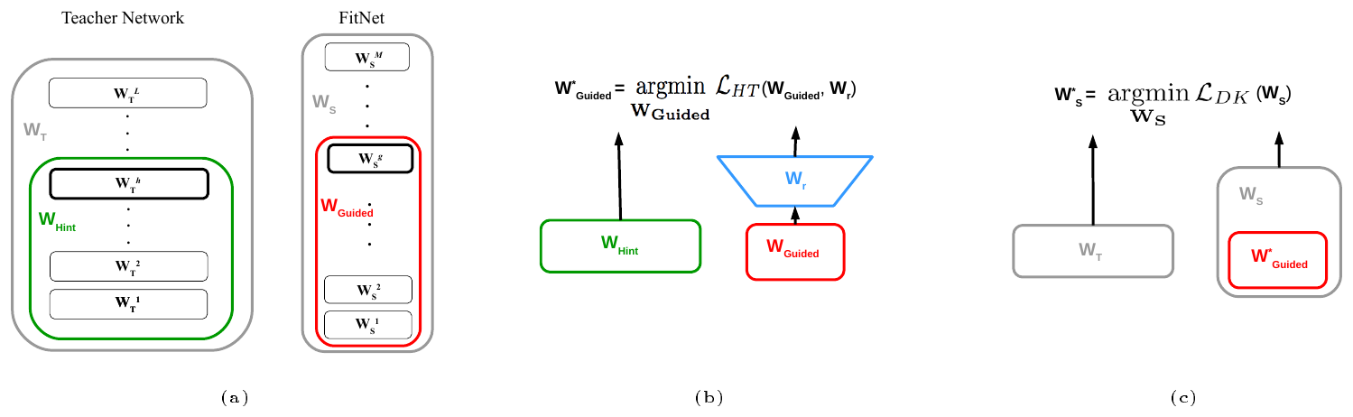
In order to help the training of deep FitNets (deeper than their teacher), we introduce hints from the teacher network. A hint is defined as the output of a teacher's hidden layer responsible for guiding the student's learning process. Analogously, we choose a hidden layer of the FitNet, the guided layer, to learn from the teacher's hint layer. We want the guided layer to be able to predict the output of the hint layer. Note that having hints is a form of regularization and thus, the pair hint/guided layer has to be chosen such that the student network is not over-regularized. The deeper we set the guided layer, the less flexibility we give to the network and, therefore, FitNets are more likely to suffer from over-regularization. In our case, we choose the hint to be the middle layer of the teacher network. Similarly, we choose the guided layer to be the middle layer of the student network.
Given that the teacher network will usually be wider than the FitNet, the selected hint layer may have more outputs than the guided layer. For that reason, we add a regressor to the guided layer, whose output matches the size of the hint layer. Then, we train the FitNet parameters from the first layer up to the guided layer as well as the regressor parameters by minimizing the following loss function:
$ \mathcal{L}{HT}(\mathbf{W{Guided}}, \mathbf{W_r}) = \frac{1}{2} || u_{h}(\mathbf{x};\mathbf{W_{Hint}}) - r(v_{g}(\mathbf{x};\mathbf{W_{Guided}});\mathbf{W_r}) ||^2,\tag{3} $
where $u_{h}$ and $v_{g}$ are the teacher/student deep nested functions up to their respective hint/guided layers with parameters $\mathbf{W_{Hint}}$ and $\mathbf{W_{Guided}}$, $r$ is the regressor function on top of the guided layer with parameters $\mathbf{W_r}$. Note that the outputs of $u_{h}$ and $r$ have to be comparable, i.e., $u_{h}$ and $r$ must be the same non-linearity.
Nevertheless, using a fully-connected regressor increases the number of parameters and the memory consumption dramatically in the case where the guided and hint layers are convolutional. Let $\mathrm{N}{h, 1} \times \mathrm{N}{h, 2}$ and $\mathrm{O}{h}$ be the teacher hint's spatial size and number of channels, respectively. Similarity, let $\mathrm{N}{g, 1} \times \mathrm{N}{g, 2}$ and $\mathrm{O}{g}$ be the FitNet guided layer's spatial size and number of channels. The number of parameters in the weight matrix of a fully connected regressor is $\mathrm{N}{h, 1} \times \mathrm{N}{h, 2} \times \mathrm{O}{h} \times \mathrm{N}{g, 1} \times \mathrm{N}{g, 2} \times \mathrm{O}{g}$. To mitigate this limitation, we use a convolutional regressor instead. The convolutional regressor is designed such that it considers approximately the same spatial region of the input image as the teacher hint. Therefore, the output of the regressor has the same spatial size as the teacher hint. Given a teacher hint of spatial size $\mathrm{N}{h, 1} \times \mathrm{N}{h, 2}$, the regressor takes the output of the Fitnet's guided layer of size $\mathrm{N}{g, 1} \times \mathrm{N}{g, 2}$ and adapts its kernel shape $\mathrm{k_1} \times \mathrm{k_2}$ such that $\mathrm{N}{g, i} - \mathrm{k}i + 1 = \mathrm{N}{h, i}$, where $i \in {1, 2}$. The number of parameters in the weight matrix of a the convolutional regressor is $\mathrm{k_1} \times \mathrm{k_2} \times \mathrm{O}{h} \times \mathrm{O}{g}$, where $\mathrm{k_1} \times \mathrm{k_2}$ is significantly lower than $\mathrm{N}{h, 1} \times \mathrm{N}{h, 2} \times \mathrm{N}{g, 1} \times \mathrm{N}_{g, 2}$.
2.3 FitNet Stage-wise Training
We train the FitNet in a stage-wise fashion following the student/teacher paradigm. Figure 1 summarizes the training pipeline. Starting from a trained teacher network and a randomly initialized FitNet (Figure 1 (a)), we add a regressor parameterized by $\mathbf{W_{r}}$ on top of the FitNet guided layer and train the FitNet parameters $\mathbf{W_{Guided}}$ up to the guided layer to minimize Eq. (3) (see Figure 1 (b)). Finally, from the pre-trained parameters, we train the parameters of whole FitNet $\mathbf{W_{S}}$ to minimize Eq. (2) (see Figure 1 (c)). Algorithm 1 details the FitNet training process.
**Input:** W(S), W(T), g, h
**Output:** W(S)*
W(Hint) ← (W(T)(1), …, W(T)(h))
W(Guided) ← (W(S)(1), …, W(S)(g))
Intialize W(r) to small random values
W(Guided)* ← argmin over W(Guided) L(HT)(W(Guided),W(r))
(W(S)(1), …, W(S)(g)) ← (W(Guided)*1, …, W(Guided)*g)
W(S)* ← argmin over W(S) L(KD)(W(S))
2.4 Relation to Curriculum Learning
In this section, we argue that our hint-based training with KD can be seen as a particular form of Curriculum Learning ([16]). Curriculum learning has proven to accelerate the training convergence as well as potentially improve the model generalization by properly choosing a sequence of training distributions seen by the learner: from simple examples to more complex ones. A curriculum learning extension ([15]) has also shown that by using guidance hints on an intermediate layer during the training, one could considerably ease training. However, [16] uses hand-defined heuristics to measure the "simplicity" of an example in a sequence and [15]'s guidance hints require some prior knowledge of the end-task. Both of these curriculum learning strategies tend to be problem-specific.
Our approach alleviates this issue by using a teacher model. Indeed, intermediate representations learned by the teacher are used as hints to guide the FitNet optimization procedure. In addition, the teacher confidence provides a measure of example "simplicity" by means of teacher cross-entropy term in Eq. (2). This term ensures that examples with a high teacher confidence have a stronger impact than examples with low teacher confidence: the latter correspond to probabilities closer to the uniform distribution, which exert less of a push on the student parameters. In other words, the teacher penalizes the training examples according to its confidence. Note that parameter $\lambda$ in Eq. (2) controls the weight given to the teacher cross-entropy, and thus, the importance given to each example. In order to promote the learning of more complex examples (examples with lower teacher confidence), we gradually anneal $\lambda$ during the training with a linear decay. The curriculum can be seen as composed of two stages: first learn intermediate concepts via the hint/guided layer transfer, then train the whole student network jointly, annealing $\lambda$, which allows easier examples (on which the teacher is very confident) to initially have a stronger effect, but progressively decreasing their importance as $\lambda$ decays. Therefore, the hint-based training introduced in the paper is a generic curriculum learning approach, where prior information about the task-at-hand is deduced purely from the teacher model.
\begin{tabular}{|c|c|c|}
 \hline
 \textbf{Algorithm} & $#$ params & \textbf{Accuracy}\\ \hline
\hline
\multicolumn{3}{|l|}{\emph{Compression}} \\ \hline
FitNet & $\sim$ 2.5M& $\mathbf{91.61\%}$ \\ \hline
Teacher & $\sim$ 9M& $90.18\%$ \\ \hline
Mimic single & $\sim$ 54M & $84.6\%$ \\ \hline
Mimic single & $\sim$ 70M & $84.9\%$ \\ \hline
Mimic ensemble & $\sim$ 70M & $85.8\%$ \\ \hline \hline
\multicolumn{3}{|l|}{\emph{State-of-the-art methods}} \\ \hline
\multicolumn{2}{|l|}{Maxout} & $90.65\%$ \\ \hline
\multicolumn{2}{|l|}{Network in Network} & $91.2\%$ \\ \hline
\multicolumn{2}{|l|}{Deeply-Supervised Networks} & $\mathbf{91.78\%}$ \\ \hline
\multicolumn{2}{|l|}{Deeply-Supervised Networks (19)} & $88.2\%$ \\ \hline
\end{tabular}
\begin{tabular}{|c|c|c|}
\hline
\textbf{Algorithm} & $#$ params & \textbf{Accuracy}\\ \hline
\hline
\multicolumn{3}{|l|}{\emph{Compression}} \\ \hline
FitNet & $\sim$ 2.5M& $\mathbf{64.96\%}$ \\ \hline
Teacher & $\sim$ 9M& $63.54\%$ \\ \hline \hline
\multicolumn{3}{|l|}{\emph{State-of-the-art methods}} \\ \hline
\multicolumn{2}{|l|}{Maxout} & $61.43\%$ \\ \hline
\multicolumn{2}{|l|}{Network in Network} & $64.32\%$ \\ \hline
\multicolumn{2}{|l|}{Deeply-Supervised Networks} & $\mathbf{65.43\%}$ \\ \hline
\end{tabular}
3. Results on Benchmark Datasets
Section Summary: The section reports experimental results showing that FitNet student models, trained with hints from larger teacher networks, achieve strong accuracy on image classification benchmarks including CIFAR-10, CIFAR-100, and SVHN. These compact students consistently match or exceed their teachers' performance while using roughly one-third as many parameters, and they outperform prior network compression techniques. The authors also demonstrate through ablations that the proposed hint-based guidance enables effective training of thin, deep architectures where direct supervision or other stage-wise methods fail.
In this section, we show the results on several benchmark datasets[^2]. The architectures of all networks as well as the training details are reported in the supplementary material.
[^2]: Code to reproduce the experiments publicly available: https://github.com/adri-romsor/FitNets
3.1 CIFAR-10 and CIFAR-100
The CIFAR-10 and CIFAR-100 datasets ([17]) are composed of 32x32 pixel RGB images belonging to 10 and 100 different classes, respectively. They both contain 50K training images and 10K test images. CIFAR-10 has 1000 samples per class, whereas CIFAR-100 has 100 samples per class. Like [18], we normalized the datasets for contrast normalization and applied ZCA whitening.
CIFAR-10: To validate our approach, we trained a teacher network of maxout convolutional layers as reported in [18] and designed a FitNet with 17 maxout convolutional layers, followed by a maxout fully-connected layer and a top softmax layer, with roughly $1/3$ of the parameters. The 11th layer of the student network was trained to mimic the 2nd layer of the teacher network. Like in [18, 14], we augmented the data with random flipping during training. Table 1 summarizes the obtained results. Our student model outperforms the teacher model, while requiring notably fewer parameters, suggesting that depth is crucial to achieve better representations. When compared to network compression methods, our algorithm achieves outstanding results; i.e., the student network achieves an accuracy of $91.61%$, which is significantly higher than the top-performer $85.8%$ of [4], while requiring roughly 28 times fewer parameters. When compared to state-of-the-art methods, our algorithm matches the best performers.
One could argue the choice of hinting the inner layers with the hidden state of a wide teacher network. A straightforward alternative would be to hint them with the desired output. This could be addressed in a few different ways: (1) Stage-wise training, where stage 1 optimizes the 1st half of the network w.r.t. classification targets and stage 2 optimizes the whole network w.r.t. classification targets. In this case, stage 1 set the network parameters in a good local minima but such initialization did not seem to help stage 2 sufficiently, which failed to learn. To further assist the training of the thin and deep student network, we could add extra hints with the desired output at different hidden layers. Nevertheless, as observed in ([11]), with supervised pre-training the guided layer may discard some factors from the input, which require more layers and non-linearity before they can be exploited to predict the classes. (2) Stage-wise training with KD, where stage 1 optimizes the 1st half of the net w.r.t. classification targets and stage 2 optimizes the whole network w.r.t. Eq. (2). As in the previous case, stage 1 set the network parameters in a good local minima but such initialization did not seem to help stage 2 sufficiently, which failed to learn. (3) Jointly optimizing both stages w.r.t. the sum of the supervised hint for the guided layer and classification target for the output layer. We performed this experiment, tried different initializations and learning rates with RMSprop ([19]) but we could not find any combination to make the network learn. Note that we could ease the training by adding hints to each layer and optimizing jointly as in Deeply Supervised Networks (DSN). Therefore, we built the above-mentioned 19-layer architecture and trained it by means of DSN, achieving a test performance of $88.2%$, which is significantly lower than the performance obtained by the FitNets hint-based training ($91.61%$). Such result suggests that using a very discriminative hint w.r.t. classification at intermediate layers might be too aggressive; using a smoother hint (such as the guidance from a teacher network) offers better generalization. (4) Jointly optimizing both stages w.r.t. the sum of supervised hint for the guided layer and Eq. (2) for the output layer. Adding supervised hints to the middle layer of the network did not ease the training of such a thin and deep network, which failed to learn.
CIFAR-100: To validate our approach, we trained a teacher network of maxout convolutional layers as reported in [18] and used the same FitNet architecture as in CIFAR-10. As in [14], we augmented the data with random flipping during training. Table 2 summarizes the obtained results. As in the previous case, our FitNet outperforms the teacher model, reducing the number of parameters by a factor of 3 and, when compared to state-of-the-art methods, the FitNet provides near state-of-the-art performance.
3.2 SVHN
The SVHN dataset ([20]) is composed by $32 \times 32$ color images of house numbers collected by GoogleStreet View. There are 73, 257 images in the training set, 26, 032 images in the test set and 531, 131 less difficult examples. We follow the evaluation procedure of [18] and use their maxout network as teacher. We trained a 13-layer FitNet composed of 11 maxout convolutional layers, a fully-connected layer and a softmax layer.
\begin{tabular}{|c|c|c|}
\hline
\textbf{Algorithm} & $#$ params & \textbf{Misclass}\\ \hline
\hline
\multicolumn{3}{|l|}{\emph{Compression}} \\ \hline
FitNet & $\sim$ 1.5M & $2.42\%$ \\ \hline
Teacher & $\sim$ 4.9M & $\mathbf{2.38\%}$ \\ \hline \hline
\multicolumn{3}{|l|}{\emph{State-of-the-art methods}} \\ \hline
\multicolumn{2}{|l|}{Maxout} & $2.47\%$ \\ \hline
\multicolumn{2}{|l|}{Network in Network} & $2.35\%$ \\ \hline
\multicolumn{2}{|l|}{Deeply-Supervised Networks} & $\mathbf{1.92\%}$ \\ \hline
\end{tabular}
\begin{tabular}{|c|c|c|}
\hline
\textbf{Algorithm} & $#$ params & \textbf{Misclass}\\ \hline
\hline
\multicolumn{3}{|l|}{\emph{Compression}} \\ \hline
Teacher & $\sim$ 361K & $0.55\%$ \\ \hline
Standard backprop & $\sim$ 30K & $1.9\%$ \\ \hline
KD & $\sim$ 30K & $0.65\%$ \\ \hline
FitNet & $\sim$ 30K & $\mathbf{0.51\%}$ \\ \hline
\multicolumn{3}{|l|}{\emph{State-of-the-art methods}} \\ \hline \hline
\multicolumn{2}{|l|}{Maxout} & $0.45\%$ \\ \hline
\multicolumn{2}{|l|}{Network in Network} & $0.47\%$ \\ \hline
\multicolumn{2}{|l|}{Deeply-Supervised Networks} & $\mathbf{0.39\%}$ \\ \hline
\end{tabular}
Table 3 shows that our FitNet achieves comparable accuracy than the teacher despite using only $32%$ of teacher capacity. Our FitNet is comparable in terms of performance to other state-of-art methods, such as Maxout and Network in Network.
3.3 MNIST
As a sanity check for the training procedure, we evaluated the proposed method on the MNIST dataset ([21]). MNIST is a dataset of handwritten digits (from 0 to 9) composed of 28x28 pixel greyscale images, with 60K training images and 10K test images. We trained a teacher network of maxout convolutional layers as reported in [18] and designed a FitNet twice as deep as the teacher network and with roughly $8%$ of the parameters. The 4th layer of the student network was trained to mimic the 2nd layer of the teacher network.
Table 4 reports the obtained results. To verify the influence of using hints, we trained the FitNet architecture using either (1) standard backprop (w.r.t. classification labels), (2) KD or (3) Hint-based Training (HT). When training the FitNet with standard backprop from the softmax layer, the deep and thin architecture achieves $1.9%$ misclassification error. Using KD, the very same network achieves $0.65%$, which confirms the potential of the teacher network; and when adding hints, the error still decreases to $0.51%$. Furthermore, the student network achieves slightly better results than the teacher network, while requiring 12 times less parameters.
3.4 AFLW
AFLW ([22]) is a real-world face database, containing 25K annotated images. In order to evaluate the proposed framework in a face recognition setting, we extracted positive samples by re-sizing the annotated regions of the images to fit 16x16 pixels patches. Similarly, we extracted 25K 16x16 pixels patches not containing faces from ImageNet ([23]) dataset, as negative samples. We used $90%$ of the extracted patches to train the network.
In this experiment, we aimed to evaluate the method on a different kind of architecture. Therefore, we trained a teacher network of 3 ReLU convolutional layers and a sigmoid output layer. We designed a first FitNet (FitNet 1) with 15 times fewer multiplications than the teacher network, and a second FitNet (FitNet 2) with 2.5 times fewer multiplications than the teacher network. Both FitNets have 7 ReLU convolutional layers and a sigmoid output layer.
The teacher network achieved $4.21%$ misclassification error on the validation set. We trained both FitNets by means of KD and HT. On the one hand, we report a misclassification error of $4.58%$ when training FitNet 1 with KD and a misclassification error of when $2.55%$ when training it with HT. On the other hand, we report a missclassifation error of $1.95%$ when training FitNet 2 with KD and a misclassification error of $1.85%$ when training it with HT. These results show how the method is extensible to different kind of architectures and highlight the benefits of using hints, especially when dealing with thinner architectures.
4. Analysis of empirical results
Section Summary: The experiments compare networks of varying depths trained on CIFAR-10 under fixed computational budgets using standard backpropagation, knowledge distillation, and hint-based training. Results show that hint-based training allows successful optimization of much deeper networks than the other methods, yielding better accuracy for a given capacity while also acting as a stronger regularizer. Overall, the resulting FitNets achieve substantial speed-ups and parameter compression relative to the teacher model, often matching or exceeding its accuracy despite far lower computational cost.
We empirically investigate the benefits of our approach by comparing various networks trained using standard backpropagation (cross-entropy w.r.t. labels), KD or Hint-based Training (HT). Experiments are performed on CIFAR-10 dataset ([17]).
We compare networks of increasing depth given a fixed computational budget. Each network is composed of successive convolutional layers of kernel size $3 \times 3$, followed by a maxout non-linearity and a non-overlapping $2 \times 2$ max-pooling. The last max-pooling takes the maximum over all remaining spatial dimensions leading to a $1 \times 1$ vector representation. We only change the depth and the number of channels per convolution between different networks, i.e. the number of channels per convolutional layer decreases as a network depth increases to respect a given computational budget.
4.1 Assisting the training of deep networks
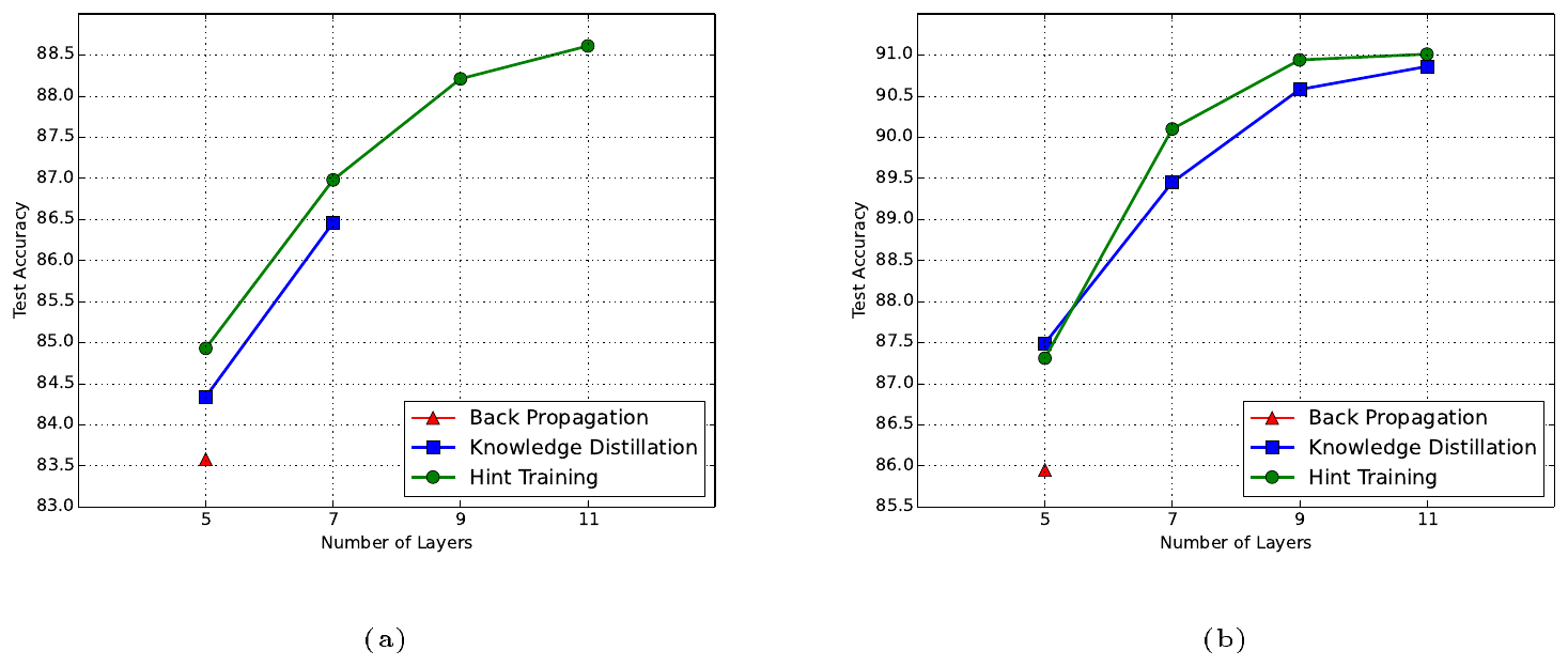
In this section, we investigate the impact of HT. We consider two computational budgets of approximately 30M and 107M operations, corresponding to the multiplications needed in an image forward propagation. For each computational budget, we train networks composed of 3, 5, 7 and 9 convolutional layers, followed by a fully-connected layer and a softmax layer. We compare their performances when they are trained with standard backpropagation, KD and HT. Figure 2 reports test on CIFAR-10 using early stopping on the validation set, i.e. we do not retrain our models on the training plus validation sets.
Due to their depth and small capacity, FitNets are hard to train. As shown in Figure 2a, we could not train 30M multiplications networks with more than 5 layers with standard backprop. When using KD, we succesfully trained networks up to 7 layers. Adding KD's teacher cross-entropy to the training objective (Eq. (2)) gives more importance to easier examples, i.e. samples for which the teacher network is confident and, can lead to a smoother version of the training cost ([16]). Despite some optimization benefits, it is worth noticing that KD training still suffers from the increasing depth and reaches its limits for 7-layer networks. HT tends to ease these optimization issues and is able to train 13-layer networks of 30M multiplications. The only difference between HT and KD is the starting point in the parameter space: either random or obtained by means of the teacher's hint. On the one hand, the proliferation of local minima and especially saddle points in highly non-linear functions such as very deep networks highlights the difficulty of finding a good starting point in the parameter space at random ([24]). On the other hand, results in Figure 2a indicate that HT can guide the student to a better initial position in the parameter space, from which we can minimize the cost through stochastic gradient descent. Therefore, HT provides benefits from an optimization point of view. Networks trained with HT also tend to yield better test performances than the other training methods when we fix the capacity and number of layers. For instance, in Figure 2b, the 7-layers network, trained with hints, obtains a $+0.7%$ performance gain on the test set compared to the model that does not use any hints (the accuracy increases from $89.45%$ to $90.1%$). As pointed by [9], pre-training strategies can act as regularizers. These results suggest that HT is a stronger regularizer than KD, since it leads to better generalization performance on the test set. Finally, Figure 2 highlights that deep models have better performances than shallower ones given a fixed computational budget. Indeed, considering networks that are trained with hints, an 11-layer network outperforms a 5-layer network by an absolute improvement of $4.11%$ for 107M multiplications and of $3.4%$ for 30M multiplications. Therefore, the experiments validate our hypothesis that given a fixed number of computations, we leverage depth in a model to achieve faster computation and better generalization.
In summary, this experiment shows that (1) using HT, we are able to train deeper models than with standard back-propagation and KD; and (2) given a fixed capacity, deeper models performed better than shallower ones.
4.2 Trade-off Between Model Performance and Efficiency
\begin{tabular}{|c|c|c|c|c|c|c|}
 \hline
 \textbf{Network} & $#$ layers & $#$ params & $#$ mult & \textbf{Acc} & \textbf{Speed-up} & \textbf{Compression rate}\\ \hline
\hline
Teacher & 5 & $\sim$ 9M & $\sim$ 725M & $90.18\%$ & 1 & 1\\ \hline
FitNet 1 & 11 & $\sim$ 250K & $\sim$ 30M & $89.01\%$ & \textbf{13.36} & \textbf{36}\\ \hline
FitNet 2 & 11 & $\sim$ 862K & $\sim$ 108M & $91.06\%$ & 4.64 & 10.44\\ \hline
FitNet 3 & 13 & $\sim$ 1.6M & $\sim$ 392M & $91.10\%$ & 1.37 & 5.62\\ \hline
FitNet 4 & 19 & $\sim$ 2.5M & $\sim$ 382M & $\mathbf{91.61\%}$ & 1.52 & 3.60\\ \hline
\end{tabular}
To evaluate FitNets efficiency, we measure their total inference times required for processing CIFAR-10 test examples on a GPU as well as their parameter compression. Table 5 reports both the speed-up and compression rate obtained by various FitNets w.r.t. the teacher model along with their number of layers, capacity and accuracies. In this experiment, we retrain our FitNets on training plus validation sets as in [18], for fair comparison with the teacher.
FitNet 1, our smallest network, with $36\times$ less capacity than the teacher, is one order of magnitude faster than the teacher and only witnesses a minor performance decrease of $1.3%$. FitNet 2, slightly increasing the capacity, outperforms the teacher by $0.9%$, while still being faster by a strong $4.64$ factor. By further increasing network capacity and depth in FitNets 3 and 4, we improve the performance gain, up to $1.6%$, and still remain faster than the teacher. Although a trade-off between speed and accuracy is introduced by the compression rate, FitNets tend to be significantly faster, matching or outperforming their teacher, even when having low capacity.
A few works such as matrix factorization ([25, 26]) focus on speeding-up deep networks'convolutional layers at the expense of slightly deteriorating their performance. Such approaches are complementary to FitNets and could be used to further speed-up the FitNet's convolutional layers.
Other works related to quantization schemes ([27, 28, 29]) aim at reducing storage requirements. Unlike FitNets, such approaches witness a little decrease in performance when compressing the network parameters. Exploiting depth allows FitNets to obtain performance improvements w.r.t. their teachers, even when reducing the number of parameters $10\times$. However, we believe that quantization approaches are also complementary to FitNets and could be used to further reduce the storage requirements. It would be interesting to compare how much redundancy is present in the filters of the teacher networks w.r.t. the filters of the FitNet and, therefore, how much FitNets filters could be compressed without witnessing significant performance drop. This analysis is out of the scope of the paper and is left as future work.
5. Conclusion
Section Summary: Researchers introduced a new method to simplify large neural networks by turning wide, high-capacity models into thinner but deeper ones, using internal guidance signals from the original network’s hidden layers to train the student model. This produces compact networks with far fewer parameters that often match or exceed the teacher’s accuracy and speed while learning strong internal features. The work suggests that future gains will come from smarter training strategies rather than simply scaling up model size.
We proposed a novel framework to compress wide and deep networks into thin and deeper ones, by introducing intermediate-level hints from the teacher hidden layers to guide the training process of the student. We are able to use these hints to train very deep student models with less parameters, which can generalize better and/or run faster than their teachers. We provided empirical evidence that hinting the inner layers of a thin and deep network with the hidden state of a teacher network generalizes better than hinting them with the classification targets. Our experiments on benchmark datasets emphasize that deep networks with low capacity are able to extract feature representations that are comparable or even better than networks with as much as 10 times more parameters. The hint-based training suggests that more efforts should be devoted to explore new training strategies to leverage the power of deep networks.
Acknowledgments
We thank the developers of Theano ([30]) and Pylearn2 ([31]) and the computational resources provided by Compute Canada and Calcul Québec. This work has been partially supported by NSERC, CIFAR, and Canada Research Chairs, Project TIN2013-41751, grant 2014-SGR-221 and Spanish MINECO grant TIN2012-38187-C03.
Appendix
Section Summary: The appendix provides supplementary details on the neural network designs and training setups used in the paper's experiments. It outlines the teacher models, which rely on maxout convolutional layers with pooling, along with the smaller FitNet student architectures built from sequences of 3x3 convolutions, maxout nonlinearities, and a few pooling stages. The text also covers initialization values, optimization via RMSProp with staged hint-based training, learning rates, epoch counts, and specific layer configurations for CIFAR and MNIST datasets that vary in depth and computational cost.
A. Supplementary Material: Network Architectures and Training Procedures
In the supplementary material, we describe all network architectures and hyper-parameters used throughout the paper.
A.1 CIFAR-10/CIFAR-100
In this section, we describe the teacher and FitNet architectures as well as hyper-parameters used in both CIFAR-10/CIFAR-100 experiments.
A.1.1 Teachers
We used the CIFAR-10/CIFAR-100 maxout convolutional networks reported in [18] as teachers. Both teachers have the same architecture, composed of 3 convolutional hidden layers of 96-192-192 units, respectively. Each convolutional layer is followed by a maxout non-linearity (with 2 linear pieces) and a max-pooling operator with respective windows sizes of 4x4, 4x4 and 2x2 pixels. All max-pooling units have an overlap of 2x2 pixels. The third convolutional layer is followed by a fully-connected maxout layer of 500 units (with 5 linear pieces) and a top softmax layer. The CIFAR-10/CIFAR-100 teachers are trained using stochastic gradient descent and momentum. Please refer to [18] for more details.
A.1.2 FitNets
Here, we describe the FitNet architectures used in the Section 3 and Section 4. Each FitNet is composed of successive zero-padded convolutional layers of kernel size $3 \times 3$, followed by a maxout non-linearity with two linear pieces. A non-overlapping $2 \times 2$ max-pooling follows some of the convolutional layers; each network has a total of 3 max-pooling units. The last max-pooling takes the maximum over all remaining spatial dimensions, leading to a $1 \times 1$ vector representation. The last convolutional layer is followed by a fully-connected and a softmax layer, as the ones on CIFAR-10/100 teachers.
Table 6 describes the architectures used for the depth experiment in Figure 2. Table 7 describes the architectures for the efficiency-performance trade-off experiment in Table 5. The results reported in Table 1, Table 2 and Table 3 correspond to the FitNet 4 architecture.
All FitNet parameters were initialized randomly in U(-0.005, 0.005). We used stochastic gradient descent with RMSProp ([19]) to train the FitNets, with an initial learning rate $0.005$ and a mini-batch size of 128. Parameter $\lambda$ in Eq. (2) was initialized to $4$ and decayed linearly during $500$ epochs reaching $\lambda = 1$. The relaxation term $\tau$ was set to 3.
On CIFAR-10, we divided the training set into 40K training examples and 10K validation examples. We trained stage 1 by minimizing Eq. (3) and stopped the training after 100 epochs of no validation error improvement, performing a maximum of 500 epochs. After that, we trained stage 2 by minimizing Eq. (2) using RMSprop, the same stopping criterion and the same hyper-parameters as stage 1. We picked the optimal number of epochs according to the above-mentioned stopping criterion and retrained the FitNet on the whole 50K training examples (training + validation sets).
On CIFAR-100, we trained directly on the whole training set using stochastic gradient descent with RMSprop, the same hyper-parameters as CIFAR-10 FitNets and the number of epochs determined by CIFAR-10 stopping criterion.
\begin{tabular}{|c|c|c|c|}
\hline
 5 Layer & 7 Layer & 9 Layer & 11 Layer\\
\hline
\hline
 conv 3x3x64 (3x3x128) & conv 3x3x16 (3x3x32) & conv 3x3x16 (3x3x32) & conv 3x3x16 (3x3x16)\\
 pool 2x2 & conv 3x3x32 (3x3x64) & conv 3x3x32 (3x3x32) & conv 3x3x16 (3x3x32)\\
  & pool 2x2 & pool 2x2 & conv 3x3x16 (3x3x32)\\
  & & & pool 2x2\\
\hline
 conv 3x3x64 (3x3x128) & conv 3x3x32 (3x3x80) & conv 3x3x32 (3x3x64) & conv 3x3x32 (3x3x48)\\
 pool 2x2 & conv 3x3x64 (3x3x80) & conv 3x3x32 (3x3x80) & conv 3x3x32 (3x3x64)\\
  & pool 2x2 & conv 3x3x32 (3x3x80) & conv 3x3x32 (3x3x80)\\
  & & pool 2x2 & pool 2x2\\
\hline
 conv 3x3x64 (3x3x128) & conv 3x3x64 (3x3x128) & conv 3x3x48 (3x3x96) & conv 3x3x48 (3x3x96)\\
 pool 8x8 & pool 8x8 & conv 3x3x64 (3x3x128) & conv 3x3x48 (3x3x96)\\
  & & pool 8x8 & conv 3x3x64 (3x3x128)\\
  & & & pool 8x8\\
\hline
 fc & fc & fc & fc \\
 softmax & softmax & softmax & softmax\\
\hline
hint: 2 $\leftarrow$ 2 & hint: 4 $\leftarrow$ 2 & hint: 5 $\leftarrow$ 2 & hint: 7 $\leftarrow$ 2\\
\hline
\end{tabular}
\begin{tabular}{|c|c|c|c|}
\hline
 FitNet 1 & FitNet 2 & FitNet 3 & FitNet 4\\
\hline
\hline
 conv 3x3x16 & conv 3x3x16 & conv 3x3x32 & conv 3x3x32\\
 conv 3x3x16 & conv 3x3x32 & conv 3x3x48 & conv 3x3x32\\
 conv 3x3x16 & conv 3x3x32 & conv 3x3x64 & conv 3x3x32\\
 pool 2x2 & pool 2x2 & conv 3x3x64 & conv 3x3x48\\
  & & pool 2x2 & conv 3x3x48\\
  & & & pool 2x2\\
\hline
 conv 3x3x32 & conv 3x3x48 & conv 3x3x80 & conv 3x3x80\\
 conv 3x3x32 & conv 3x3x64 & conv 3x3x80 & conv 3x3x80\\
 conv 3x3x32 & conv 3x3x80 & conv 3x3x80 & conv 3x3x80\\
 pool 2x2 & pool 2x2 & conv 3x3x80 & conv 3x3x80\\
  & & pool 2x2 & conv 3x3x80\\
  & & & conv 3x3x80\\
  & & & pool 2x2\\
\hline
 conv 3x3x48 & conv 3x3x96 & conv 3x3x128 & conv 3x3x128\\
 conv 3x3x48 & conv 3x3x96 & conv 3x3x128 & conv 3x3x128\\
 conv 3x3x64 & conv 3x3x128 & conv 3x3x128 & conv 3x3x128\\
 pool 8x8 & pool 8x8 & pool 8x8 & conv 3x3x128\\
  & & & conv 3x3x128\\
  & & & conv 3x3x128\\
  & & & pool 8x8\\
\hline
 fc & fc & fc & fc\\
 softmax & softmax & softmax & softmax\\
\hline
hint: 6 $\leftarrow$ 2 & hint: 6 $\leftarrow$ 2 & hint: 8 $\leftarrow$ 2 & hint: 11 $\leftarrow$ 2\\
\hline
\end{tabular}
A.2 MNIST
In this section, we describe the teacher and FitNet architectures as well as the hyper-parameters used in the MNIST experiments.
We trained a teacher network of maxout convolutional layers as reported in [18]. The teacher architecture has three convolutional maxout hidden layers (with 2 linear pieces each) of 48-48-24 units, respectively, followed by a spatial max-pooling of 4x4-4x4-2x2 pixels, with an overlap of 2x2 pixels. The 3rd hidden layer is followed by a fully-connected softmax layer. As is [18], we added zero padding to the second convolutional layer.
We designed a FitNet twice as deep as the teacher network and with roughly $8%$ of the parameters. The student architecture has 6 maxout convolutional hidden layers (with 2 linear pieces each) of 16-16-16-16-12-12 units, respectively. Max-pooling is only applied every second layer in regions of 4x4-4x4-2x2 pixels, with an overlap of 2x2 pixels. The 6th convolutional hidden layer is followed by a fully-connected softmax layer.
The teacher network was trained as described in [18]. The FitNet was trained in a stage-wise fashion as described in Section 2. We divided the training set into a training set of 50K samples and a validation set of 10K samples.
All network parameters where initialized randomly in U(-0.005, 0.005). In the first stage, the 4th layer of the FitNet was trained to mimic the 2nd layer of the teacher network, by minimizing Eq. (3) through stochastic gradient descent. We used a mini-batch size of 128 samples and fixed the learning rate to 0.0005. We initialized $\lambda$ to 4 and decayed it for the first 150 epochs until it reached 1. The training was stopped according to the following criterion: after 100 epochs of no validation error improvement and performning a maximum of 500 epochs. We used the same mini-batch size, learning rate and stopping criterion to train the second stage. The relaxation term $\tau$ was set to 3.
A.3 SVHN
In this section, we describe the teacher and FitNet architectures as well as the hyper-parameters used in the SVHN experiments.
We used SVHN maxout convolutional network described in as [18] teacher. The network is composed of 3 convolutional hidden layers of 64-128-128 units, respectively, followed by a fully-connected maxout layer of 400 units and a top softmax layer. The teacher training was carried out as in [18].
We used the FitNet 4 architecture outlined in Table 7, initializing the network parameters randomly in U(-0.005, 0.005) and training with the same hyper-parameters as in CIFAR-10. In this case, we used the same early stopping as in CIFAR-10, but we did not retrain the FitNet on the whole training set (training + validation). The same hyper-parameters where used for both stages.
A.4 AFLW
In this section, we describe the teacher and FitNet architectures as well as the hyper-parameters used in the AFLW experiments.
We trained a teacher network of 3 ReLU convolutional layers of 128-512-512 units, respectively, followed by a sigmoid layer. Non-overlapping max-pooling of size $2 \times 2$ was performed after the first convolutional layer. We used receptive fields of 3-2-5 for each layer, respectively.
We designed two FitNets of 7 ReLU convolutional layers. Fitnet 1's layers have 16-32-32-32-32-32-32-32 units, respectively, followed by a sigmoid layer. Fitnet 2's layers have 32-64-64-64-64-64-64-64 units, respectively, followed by a sigmoid layer. In both cases, we used receptive fields of $3 \times 3$ and, due to the really small image resolution, we did not perform any max-pooling.
All network parameters of both FitNets where initialized randomly in U(-0.05, 0.05). Both FitNets were trained in the stage-wise fashion described in Section 2. We used $90%$ of the data for training. In the first stage, the 5th layer of the FitNets were trained to mimic the 3rd layer of the teacher network, by minimizing Eq. (3) through stochastic gradient descent. We used a mini-batch size of 128 samples and initialized the learning rate to 0.001 and decayed it for the first 100 epochs until reaching 0.01. We also used momentum. We initialized momentum to 0.1 and saturated it to 0.9 at epoch 100. We picked the best validation value after a 500 epochs. We used the same mini-batch size, learning rate and stopping criterion to train the second stage. The relaxation term $\tau$ was set to 3.
References
Section Summary: This section compiles a list of academic papers, theses, and technical resources that the authors cite as foundational or related work. The references center on deep neural networks and convolutional architectures for image recognition tasks, along with techniques for model compression, knowledge distillation, and efficient training of large models. They also cover supporting topics such as representation learning, optimization challenges, benchmark datasets like ImageNet and CIFAR, and open-source tools for machine learning experiments.
[1] Simonyan, K. and Zisserman, A. Very deep convolutional networks for large-scale image recognition. CoRR, abs/1409.1556, 2014.
[2] Szegedy, C., Liu, W., Jia, Y., Sermanet, P., Reed, S., D.A., Erhan, D., Vanhoucke, V., and Rabinovich, A. Going deeper with convolutions. CoRR, abs/1409.4842, 2014.
[3] Bucila, C., Caruana, R., and Niculescu-Mizil, A. Model compression. In KDD, pp. 535–541, 2006.
[4] Ba, J. and Caruana, R. Do deep nets really need to be deep? In NIPS, pp. 2654–2662. 2014.
[5] Hinton, G. Vinyals, O. and Dean, J. Distilling knowledge in a neural network. In Deep Learning and Representation Learning Workshop, NIPS, 2014.
[6] Bengio, Y., Courville, A., and Vincent, P. Representation learning: A review and new perspectives. TPAMI, 2013.
[7] Montufar, G.F., Pascanu, R., Cho, K., and Bengio, Y. On the number of linear regions of deep neural networks. In NIPS. 2014.
[8] Larochelle, H., Erhan, D., Courville, A., Bergstra, J., and Bengio, Y. An empirical evaluation of deep architectures on problems with many factors of variation. In ICML, pp. 473–480, 2007.
[9] Erhan, D., Manzagol, P.A., Bengio, Y., Bengio, S., and Vincent, P. The difficulty of training deep architectures and the effect of unsupervised pre-training. In AISTATS, pp. 153–160, 2009.
[10] Hinton, G. E., Osindero, S., and Teh, Y.-W. A fast learning algorithm for deep belief nets. Neural Computation, 18(7):1527–1554, 2006.
[11] Bengio, Y., Lamblin, P., Popovici, D., and Larochelle, H. Greedy layer-wise training of deep networks. In NIPS, pp. 153–160, 2007.
[12] Weston, J., Ratle, F., and Collobert, R. Deep learning via semi-supervised embedding. In ICML, 2008.
[13] Cho, Kyunghyun, Raiko, Tapani, Ilin, Alexander, and Karhunen, Juha. A two-stage pretraining algorithm for deep Boltzmann machines. In NIPS Workshop on Deep Learning and Unsupervised Feature Learning, 2012.
[14] Chen-Yu, L., Saining, X., Patrick, G., Zhengyou, Z., and Zhuowen, T. Deeply-supervised nets. CoRR, abs/1409.5185, 2014.
[15] Gulcehre, C. and Bengio, Y. Knowledge matters: Importance of prior information for optimization. In ICLR, 2013.
[16] Bengio, Y. Learning deep architectures for AI. Foundations and trends in Machine Learning, 2009.
[17] Krizhevsky, A. and Hinton, G. Learning multiple layers of features from tiny images. Master's thesis, Department of Computer Science, University of Toronto, 2009.
[18] Goodfellow, I.J., Warde-Farley, D., Mirza, M., Courville, A., and Bengio, Y. Maxout networks. In ICML, 2013b.
[19] Tieleman, T. and Hinton, G. Lecture 6.5—RmsProp: Divide the gradient by a running average of its recent magnitude. COURSERA: Neural Networks for Machine Learning, 2012.
[20] Netzer, Y., Wang, T., Coates, A., Bissacco, A., Wu, B., and Ng, A. Reading digits in natural images with unsupervised feature learning. In Deep Learning & Unsupervised Feature Learning Workshop, NIPS, 2011.
[21] LeCun, Y., Bottou, L., Bengio, Y., and Haffner, P. Gradient-based learning applied to document recognition. Proceedings of the IEEE, 86(11):2278–2324, November 1998.
[22] Koestinger, M., Wohlhart, P., Roth, P.M., and Bischof, H. Annotated facial landmarks in the wild: A large-scale, real-world database for facial landmark localization. In First IEEE International Workshop on Benchmarking Facial Image Analysis Technologies, 2011.
[23] Russakovsky, O., Deng, J., Su, H., Krause, J., Satheesh, S., Ma, S., Huang, Z., Karpathy, A., Khosla, A., Bernstein, M., Berg, A. C., and Fei-Fei, L. ImageNet Large Scale Visual Recognition Challenge, 2014.
[24] Dauphin, Y., Pascanu, R., Gulcehre, C., Cho, K., Ganguli, S., and Bengio, Y. Identifying and attacking the saddle point problem in high-dimensional non-convex optimization. In NIPS, 2014.
[25] Jaderberg, M., Vedaldi, A., and Zisserman, A. Speeding up convolutional neural networks with low rank expansions. In BMVC, 2014.
[26] Denton, Emily L, Zaremba, Wojciech, Bruna, Joan, LeCun, Yann, and Fergus, Rob. Exploiting linear structure within convolutional networks for efficient evaluation. In NIPS, pp. 1269–1277. 2014.
[27] Chen, Yongjian, Guan, Tao, and Wang, Cheng. Approximate nearest neighbor search by residual vector quantization. Sensors, 10(12):11259–11273, 2010.
[28] Jégou, Hervé, Douze, Matthijs, and Schmid, Cordelia. Product quantization for nearest neighbor search. IEEE TPAMI, 33(1):117–128, 2011.
[29] Gong, Yunchao, Liu, Liu, Yang, Min, and Bourdev, Lubomir. Compressing deep convolutional networks using vector quantization. CoRR, abs/1412.6115, 2014.
[30] Bastien, F., Lamblin, P., Pascanu, R., Bergstra, J., Goodfellow, I., Bergeron, A., Bouchard, N., Warde-Farley, D., and Bengio, Y. Theano: new features and speed improvements. Deep Learning & Unsupervised Feature Learning Workshop, NIPS, 2012.
[31] Goodfellow, I. J., Warde-Farley, D., Lamblin, P., Dumoulin, V., Mirza, M., Pascanu, R., Bergstra, J., Bastien, F., and Bengio, Y. Pylearn2: a machine learning research library. arXiv preprint arXiv:1308.4214, 2013a.