Can You Trust Your Model's Uncertainty? Evaluating Predictive Uncertainty Under Dataset Shift

Yaniv Ovadia$^{*}$
Google Research
[email protected]

Emily Fertig$^{*\dagger}$
Google Research
[email protected]

Jie Ren$^{\dagger}$
Google Research
[email protected]

Zachary Nado
Google Research
[email protected]

D Sculley
Google Research
[email protected]

Sebastian Nowozin
Google Research
[email protected]

Joshua V. Dillon
Google Research
[email protected]

Balaji Lakshminarayanan$^{\ddagger}$
DeepMind
[email protected]

Jasper Snoek$^{\ddagger}$
Google Research
[email protected]

Abstract

Modern machine learning methods including deep learning have achieved great success in predictive accuracy for supervised learning tasks, but may still fall short in giving useful estimates of their predictive uncertainty. Quantifying uncertainty is especially critical in real-world settings, which often involve input distributions that are shifted from the training distribution due to a variety of factors including sample bias and non-stationarity. In such settings, well calibrated uncertainty estimates convey information about when a model's output should (or should not) be trusted. Many probabilistic deep learning methods, including Bayesian-and non-Bayesian methods, have been proposed in the literature for quantifying predictive uncertainty, but to our knowledge there has not previously been a rigorous large-scale empirical comparison of these methods under dataset shift. We present a large-scale benchmark of existing state-of-the-art methods on classification problems and investigate the effect of dataset shift on accuracy and calibration. We find that traditional post-hoc calibration does indeed fall short, as do several other previous methods. However, some methods that marginalize over models give surprisingly strong results across a broad spectrum of tasks.

Executive Summary: Machine learning models, particularly deep neural networks, power critical applications like medical diagnostics and self-driving cars. However, these models often face dataset shift in real life—when incoming data differs from training data due to factors like changing trends or biases. This shift can degrade predictions and make confidence scores unreliable, increasing risks in high-stakes decisions. Reliable uncertainty estimates help users know when to trust or ignore a model's output, preventing errors in safety-sensitive areas where data distributions are rarely stable.

This document evaluates how well various methods quantify predictive uncertainty in deep learning models under dataset shift. It compares established techniques to determine which provide trustworthy confidence levels when data changes.

The authors conducted a large-scale benchmark, testing methods on classification tasks across image (CIFAR-10, ImageNet, MNIST), text (20 Newsgroups), and categorical (Criteo ad-click) datasets. They trained models following standard protocols, then assessed performance on shifted data—such as rotated or blurred images, reassigned text categories, or randomized features—and fully out-of-distribution (OOD) sets like unrelated images or text corpora. Key methods included basic softmax predictions, post-hoc temperature scaling for calibration, Monte Carlo dropout, deep ensembles of multiple models, and variational inference approximations. Metrics focused on accuracy, calibration (how well confidence matches actual error rates), Brier score (balancing sharpness and calibration), and entropy (uncertainty levels). Experiments covered thousands of examples, with hyperparameters tuned via optimization, emphasizing practical scalability without deep technical tweaks.

The most important findings reveal stark differences in method robustness. First, deep ensembles—training 5 to 10 independent models and averaging predictions—consistently outperformed others, maintaining 20-40% better calibration and accuracy under moderate to high shift compared to single models, across all datasets. Second, post-hoc temperature scaling calibrated well on matching test data (reducing expected calibration error by up to 50%) but failed dramatically under shift, worsening Brier scores by 10-30% as data diverged. Third, dropout methods improved uncertainty over basic models, yielding higher entropy on OOD data (about 20% more than vanilla approaches), but last-layer variants underperformed, often being more overconfident on shifts. Fourth, stochastic variational inference showed promise on simple datasets like MNIST (best Brier score under heavy shift) but scaled poorly, degrading on complex ones like ImageNet. Finally, no method perfectly detected OOD inputs; most remained overconfident, with ensembles producing the highest but still imperfect entropy separation (only 30-50% better than baselines).

These results mean that standard calibration techniques, tuned on training-like data, cannot ensure reliable uncertainty in deployed systems where shifts are common, potentially leading to undetected errors in costs, safety, or compliance—such as misdiagnoses rising 2-3 times under mild perturbations. Ensembles capture epistemic uncertainty (model ignorance) effectively, enabling better risk assessment and selective use of predictions, but they differ from prior i.i.d.-focused studies, which overstated simpler methods' value. This highlights a gap: models may seem trustworthy in labs but falter in dynamic real-world settings.

Decision-makers should prioritize deep ensembles for new projects, as they offer the best trade-off in performance with modest added compute (5-10 models suffice for most gains). Avoid relying solely on post-hoc scaling for shift-prone applications. Next steps include piloting ensembles on domain-specific data to confirm benefits, then investing in research to reduce their computational costs (2-10 times higher than single models) while improving OOD detection. Further benchmarks on emerging shifts, like adversarial inputs, would strengthen guidance.

Limitations include the focus on scalable methods only, excluding some generative or OOD-specific techniques, and challenges scaling variational inference on large datasets, which may bias comparisons. Assumptions like fixed shift types limit generality, and results vary by architecture (e.g., convolutional vs. recurrent). Overall confidence is high for ensembles' superiority on tested tasks, but caution is needed for unexamined domains; more real-world validation is essential before broad adoption.

1. Introduction

Section Summary: Deep neural networks are now commonly used in critical areas like medical imaging and self-driving cars, where they not only predict outcomes but also need to provide reliable confidence levels to handle risks. However, real-world data often changes from what the models were trained on, making it essential to evaluate how well these confidence estimates hold up under such shifts, as traditional calibration methods can fail in these scenarios. This paper introduces a comprehensive benchmark that tests popular uncertainty quantification techniques across image, text, and other data types, both in standard settings and under data shifts, while sharing open-source code for further research.

Recent successes across a variety of domains have led to the widespread deployment of deep neural networks (DNNs) in practice. Consequently, the predictive distributions of these models are increasingly being used to make decisions in important applications ranging from machine-learning aided medical diagnoses from imaging ([1]) to self-driving cars ([2]). Such high-stakes applications require not only point predictions but also accurate quantification of predictive uncertainty, i.e. meaningful confidence values in addition to class predictions. With sufficient independent labeled samples from a target data distribution, one can estimate how well a model's confidence aligns with its accuracy and adjust the predictions accordingly. However, in practice, once a model is deployed the distribution over observed data may shift and eventually be very different from the original training data distribution. Consider, e.g., online services for which the data distribution may change with the time of day, seasonality or popular trends. Indeed, robustness under conditions of distributional shift and out-of-distribution (OOD) inputs is necessary for the safe deployment of machine learning ([3]). For such settings, calibrated predictive uncertainty is important because it enables accurate assessment of risk, allows practitioners to know how accuracy may degrade, and allows a system to abstain from decisions due to low confidence.

A variety of methods have been developed for quantifying predictive uncertainty in DNNs. Probabilistic neural networks such as mixture density networks ([4]) capture the inherent ambiguity in outputs for a given input, also referred to as aleatoric uncertainty ([5]). Bayesian neural networks learn a posterior distribution over parameters that quantifies parameter uncertainty, a type of epistemic uncertainty that can be reduced through the collection of additional data. Popular approximate Bayesian approaches include Laplace approximation ([6]), variational inference ([7, 8]), dropout-based variational inference ([9, 10]), expectation propagation [11] and stochastic gradient MCMC ([12]). Non-Bayesian methods include training multiple probabilistic neural networks with bootstrap or ensembling ([13, 14]). Another popular non-Bayesian approach involves re-calibration of probabilities on a held-out validation set through temperature scaling ([15]), which was shown by [16] to lead to well-calibrated predictions on the i.i.d. test set.

Using Distributional Shift to Evaluate Predictive Uncertainty While previous work has evaluated the quality of predictive uncertainty on OOD inputs ([14]), there has not to our knowledge been a comprehensive evaluation of uncertainty estimates from different methods under dataset shift. Indeed, we suggest that effective evaluation of predictive uncertainty is most meaningful under conditions of distributional shift. One reason for this is that post-hoc calibration gives good results in independent and identically distributed (i.i.d.) regimes, but can fail under even a mild shift in the input data. And in real world applications, as described above, distributional shift is widely prevalent. Understanding questions of risk, uncertainty, and trust in a model's output becomes increasingly critical as shift from the original training data grows larger.

Contributions In the spirit of calls for more rigorous understanding of existing methods ([17, 18, 19]), this paper provides a benchmark for evaluating uncertainty that focuses not only on the i.i.d. setting but also uncertainty under distributional shift. We present a large-scale evaluation of popular approaches in probabilistic deep learning, focusing on methods that operate well in large-scale settings, and evaluate them on a diverse range of classification benchmarks across image, text, and categorical modalities. We use these experiments to evaluate the following questions:

• How trustworthy are the uncertainty estimates of different methods under dataset shift?
• Does calibration in the i.i.d. setting translate to calibration under dataset shift?
• How do uncertainty and accuracy of different methods co-vary under dataset shift? Are there methods that consistently do well in this regime?

In addition to answering the questions above, our code is made available open-source along with our model predictions such that researchers can easily evaluate their approaches on these benchmarks ^1.

2. Background

Section Summary: This section explains the basic setup for a classification problem using neural networks, where features and labels from a training dataset help the model learn to predict labels from the true underlying data distribution, which is unknown and observed only through samples. At testing, the model is evaluated on similar data but also on out-of-distribution (OOD) inputs, including slightly altered versions of the original data that should increase prediction uncertainty, and entirely new data with unfamiliar labels, where the goal is to detect higher uncertainty without needing true labels. It overviews existing methods for better uncertainty estimation and OOD detection, such as those focusing solely on label predictions given features, joint modeling of features and labels, or adding OOD-specific components, but emphasizes comparing methods with similar assumptions about the data to ensure fairness.

Notation and Problem Setup Let ${\bm{x}}\in \mathbb{R}^d$ represent a set of $d$-dimensional features and $y\in{1, \ldots, k}$ denote corresponding labels (targets) for $k$-class classification. We assume that a training dataset $\mathcal{D}$ consists of $N$ i.i.d. samples $\mathcal{D}={({\bm{x}}n, y_n)}{n=1}^N$.

Let $p^*({\bm{x}}, y)$ denote the true distribution (unknown, observed only through the samples $\mathcal{D}$), also referred to as the data generating process. We focus on classification problems, in which the true distribution is assumed to be a discrete distribution over $k$ classes, and the observed $y\in{1, \ldots, k}$ is a sample from the conditional distribution $p^*(y| {\bm{x}})$. We use a neural network to model $p_{\bm{\theta}}(y| {\bm{x}})$ and estimate the parameters ${\bm{\theta}}$ using the training dataset. At test time, we evaluate the model predictions against a test set, sampled from the same distribution as the training dataset. However, here we also evaluate the model against OOD inputs sampled from $q({\bm{x}}, y) \neq p^*({\bm{x}}, y) $. In particular, we consider two kinds of shifts:

• shifted versions of the test inputs where the ground truth label belongs to one of the $k$ classes. We use shifts such as corruptions and perturbations proposed by [20], and ideally would like the model predictions to become more uncertain with increased shift, assuming shift degrades accuracy. This is also referred to as covariate shift ([21]).
• a completely different OOD dataset, where the ground truth label is not one of the $k$ classes. Here we check if the model exhibits higher predictive uncertainty for those new instances and to this end report diagnostics that rely only on predictions and not ground truth labels.

High-level overview of existing methods A large variety of methods have been developed to either provide higher quality uncertainty estimates or perform OOD detection to inform model confidence. These can roughly be divided into:

1. Methods which deal with $p(y| {\bm{x}})$ only, we discuss these in more detail in Section 3.
2. Methods which model the joint distribution $p(y, {\bm{x}})$, e.g. deep hybrid models ([22, 23, 24, 25]).
3. Methods with an OOD-detection component in addition to $p(y| {\bm{x}})$ ([26, 27, 28]), and related work on selective classification ([29]). }

We refer to [30] for a recent summary of these methods. Due to the differences in modeling assumptions, a fair comparison between these different classes of methods is challenging; for instance, some OOD detection methods rely on knowledge of a known OOD set, or train using a none-of-the-above class, and it may not always be meaningful to compare predictions from these methods with those obtained from a Bayesian DNN. We focus on methods described by (1) above, as this allows us to focus on methods which make the same modeling assumptions about data and differ only in how they quantify predictive uncertainty.

3. Methods and Metrics

Section Summary: This section outlines several common methods from probabilistic deep learning, such as maximum softmax probability, temperature scaling, Monte-Carlo dropout, neural network ensembles, and variational inference approaches, chosen for their widespread use, ability to handle large datasets, and practical value in estimating prediction uncertainty. It also describes key evaluation metrics beyond basic accuracy, including negative log-likelihood and Brier score, which are reliable ways to assess how well a model's predicted probabilities match real outcomes, though they have limitations like over-focusing on rare events; expected calibration error checks if confidence levels align with actual accuracy using data bins. For out-of-distribution inputs without true labels, the section uses visualizations like confidence histograms, entropy measures, and accuracy plots filtered by confidence thresholds to gauge model reliability.

We select a subset of methods from the probabilistic deep learning literature for their prevalence, scalability and practical applicability[^2]. These include (see also references within):

[^2]: The methods used scale well for training and prediction (see in Appendix A.9.). We also explored methods such as scalable extensions of Gaussian Processes ([31]), but they were challenging to train on the 37M example Criteo dataset or the 1000 classes of ImageNet.

• (Vanilla) Maximum softmax probability ([32])

• (Temp Scaling) Post-hoc calibration by temperature scaling using a validation set ([16])

• (Dropout) Monte-Carlo Dropout ([9, 33]) with rate $p$

• (Ensembles) Ensembles of $M$ networks trained independently on the entire dataset using random initialization ([14]) (we set $M=10$ in experiments below)

• (SVI) Stochastic Variational Bayesian Inference for deep learning ([8, 7, 34, 35, 36]). We refer to Appendix A.6 for details of our SVI implementation.

• (LL) Approx. Bayesian inference for the parameters of the last layer only ([37])

  • (LL SVI) Mean field stochastic variational inference on the last layer only
  • (LL Dropout) Dropout only on the activations before the last layer

In addition to metrics (we use arrows to indicate which direction is better) that do not depend on predictive uncertainty, such as classification accuracy $\uparrow$, the following metrics are commonly used:

Negative Log-Likelihood (NLL) $\downarrow$ Commonly used to evaluate the quality of model uncertainty on some held out set. Drawbacks: Although a proper scoring rule ([38]), it can over-emphasize tail probabilities ([39]).

Brier Score $\downarrow$ ([40]) Proper scoring rule for measuring the accuracy of predicted probabilities. It is computed as the squared error of a predicted probability vector, $p(y|x_n, {\bm{\theta}})$, and the one-hot encoded true response, $y_n$. That is,

$ \mathrm{BS} = |\mathcal{Y}|^{-1} \sum_{y\in\mathcal{Y}} (p(y| {\bm{x}}_n, {\bm{\theta}}) - \delta(y-y_n))^2 = |\mathcal{Y}|^{-1}\Big(1- 2 p(y_n| {\bm{x}}n, {\bm{\theta}})+\sum{y\in\mathcal{Y}} p(y| {\bm{x}}_n, {\bm{\theta}})^2\Big). $

The Brier score has a convenient interpretation as $BS = \mathrm{uncertainty} - \mathrm{resolution} + \mathrm{reliability}$, where $\mathrm{uncertainty}$ is the marginal uncertainty over labels, $\mathrm{resolution}$ measures the deviation of individual predictions against the marginal, and $\mathrm{reliability}$ measures calibration as the average violation of long-term true label frequencies. We refer to [41] for the decomposition of Brier score into calibration and refinement for classification and to ([42]) for the general decomposition for any proper scoring rule. Drawbacks: Brier score is insensitive to predicted probabilities associated with in/frequent events.

Both the Brier score and the negative log-likelihood are proper scoring rules and therefore the optimum score corresponds to a perfect prediction. In addition to these two metrics, we also evaluate two metrics—expected calibration error and entropy. Neither of these is a proper scoring rule, and thus there exist trivial solutions which yield optimal scores; for example, returning the marginal probability $p(y)$ for every instance will yield perfectly calibrated but uninformative predictions. Each proper scoring rule induces a calibration measure ([42]). However, ECE is not the result of such decomposition and has no corresponding proper scoring rule; we instead include ECE because it is popularly used and intuitive. Each proper scoring rule is also associated with a corresponding entropy function and Shannon entropy is that for log probability ([38]).

Expected Calibration Error (ECE) $\downarrow$ Measures the correspondence between predicted probabilities and empirical accuracy ([43]). It is computed as the average gap between within bucket accuracy and within bucket predicted probability for $S$ buckets $B_s = {n \in 1\ldots N : p(y_n| {\bm{x}}n, {\bm{\theta}}) \in (\rho_s, \rho{s+1}]}$. That is, $\mathrm{ECE} = \sum_{s=1}^S \frac{|B_s|}{N} |\operatorname{acc}(B_s) - \operatorname{conf}(B_s)|, $ where $\operatorname{acc}(B_s) = |B_s|^{-1}\sum_{n\in B_s} [y_n = \hat{y}n]$, $\operatorname{conf}(B_s)=|B_s|^{-1}\sum{n\in B_s} p(\hat{y}_n| {\bm{x}}_n, {\bm{\theta}})$, and $\hat{y}_n=\arg\max_y p(y| {\bm{x}}_n, {\bm{\theta}})$ is the $n$-th prediction. When bins ${\rho_s : s\in 1\ldots S}$ are quantiles of the held-out predicted probabilities, $|B_s|\approx|B_k|$ and the estimation error is approximately constant. Drawbacks: Due to binning, ECE does not monotonically increase as predictions approach ground truth. If $|B_s|\ne |B_k|$, the estimation error varies across bins.

There is no ground truth label for fully OOD inputs. Thus we report histograms of confidence and predictive entropy on known and OOD inputs and accuracy versus confidence plots ([14]): Given the prediction $p(y=k| {\bm{x}}_n, {\bm{\theta}})$, we define the predicted label as $\hat{y}_n=\arg\max_y p(y| {\bm{x}}_n, {\bm{\theta}})$, and the confidence as $p(y=\hat{y}| {\bm{x}}, {\bm{\theta}}) = \max_k p(y=k| {\bm{x}}_n, {\bm{\theta}})$. We filter out test examples corresponding to a particular confidence threshold $\tau\in[0, 1]$ and compute the accuracy on this set.

4. Experiments and Results

Section Summary: Researchers tested how well deep learning models handle uncertainty in predictions across image, text, and ad data, using standard training methods plus versions of data that were altered or completely different to simulate real-world changes. On the simple MNIST handwriting dataset, they found that while all models lost accuracy on altered data, a method called SVI stayed more reliable by showing higher uncertainty and avoiding overconfident wrong answers, unlike others that seemed too sure even on unfamiliar inputs. For larger image sets like CIFAR-10 and ImageNet, similar patterns emerged with distorted images, where most models struggled to adapt their confidence levels under shifts, highlighting the need for better uncertainty awareness.

We evaluate the behavior of the predictive uncertainty of deep learning models on a variety of datasets across three different modalities: images, text and categorical (online ad) data. For each we follow standard training, validation and testing protocols, but we additionally evaluate results on increasingly shifted data and an OOD dataset. We detail the models and implementations used in Appendix A. Hyperparameters were tuned for all methods using Bayesian optimization ([44]) (except on ImageNet) as detailed in Appendix A.8.

4.1 An illustrative example - MNIST

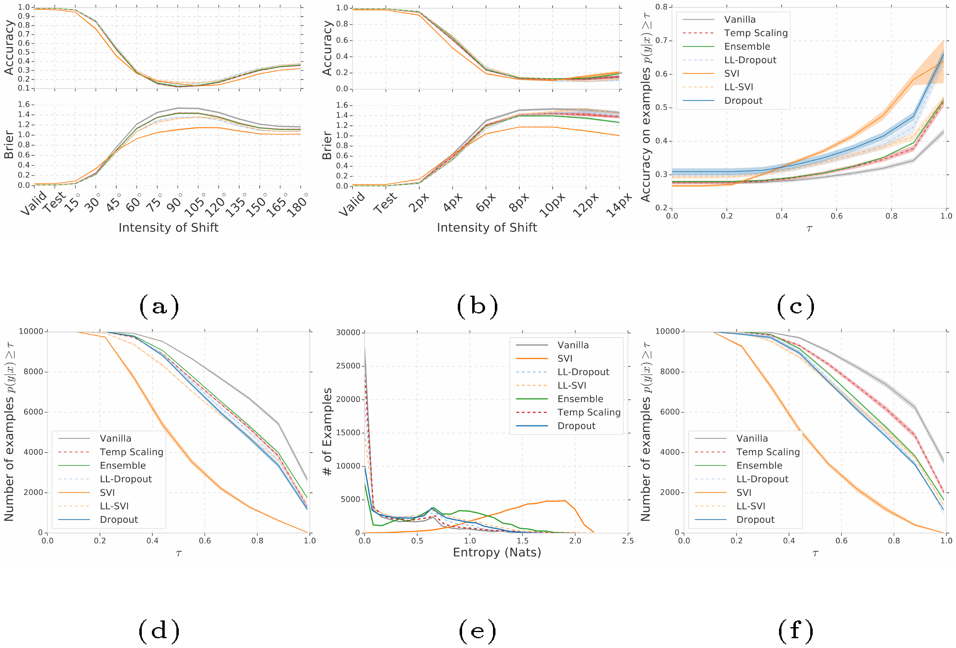
We first illustrate the problem setup and experiments using the MNIST dataset. We used the LeNet ([45]) architecture, and, as with all our experiments, we follow standard training, validation, testing and hyperparameter tuning protocols. However, we also compute predictions on increasingly shifted data (in this case increasingly rotated or horizontally translated images) and study the behavior of the predictive distributions of the models. In addition, we predict on a completely OOD dataset, Not-MNIST ([46]), and observe the entropy of the model's predictions. We summarize some of our findings in Figure 1 and discuss below.

What we would like to see: Naturally, we expect the accuracy of a model to degrade as it predicts on increasingly shifted data, and ideally this reduction in accuracy would coincide with increased forecaster entropy. A model that was well-calibrated on the training and validation distributions would ideally remain so on shifted data. If calibration (ECE or Brier reliability) remained as consistent as possible, practitioners and downstream tasks could take into account that a model is becoming increasingly uncertain. On the completely OOD data, one would expect the predictive distributions to be of high entropy. Essentially, we would like the predictions to indicate that a model "knows what it does not know" due to the inputs straying away from the training data distribution.

What we observe: We see in Figure 1a and Figure 1b that accuracy certainly degrades as a function of shift for all methods tested, and they are difficult to disambiguate on that metric. However, the Brier score paints a clearer picture and we see a significant difference between methods, i.e. prediction quality degrades more significantly for some methods than others. An important observation is that while calibrating on the validation set leads to well-calibrated predictions on the test set, it does not guarantee calibration on shifted data. In fact, nearly all other methods (except vanilla) perform better than the state-of-the-art post-hoc calibration (Temperature scaling) in terms of Brier score under shift. While SVI achieves the worst accuracy on the test set, it actually outperforms all other methods by a much larger margin when exposed to significant shift. In Figure 1c and Figure 1d we look at the distribution of confidences for each method to understand the discrepancy between metrics. We see in Figure 1d that SVI has the lowest confidence in general but in Figure 1c we observe that SVI gives the highest accuracy at high confidence (or conversely is much less frequently confidently wrong), which can be important for high-stakes applications. Most methods demonstrate very low entropy (Figure 1e) and give high confidence predictions (Figure 1f) on data that is entirely OOD, i.e. they are confidently wrong about completely OOD data.

4.2 Image Models: CIFAR-10 and ImageNet

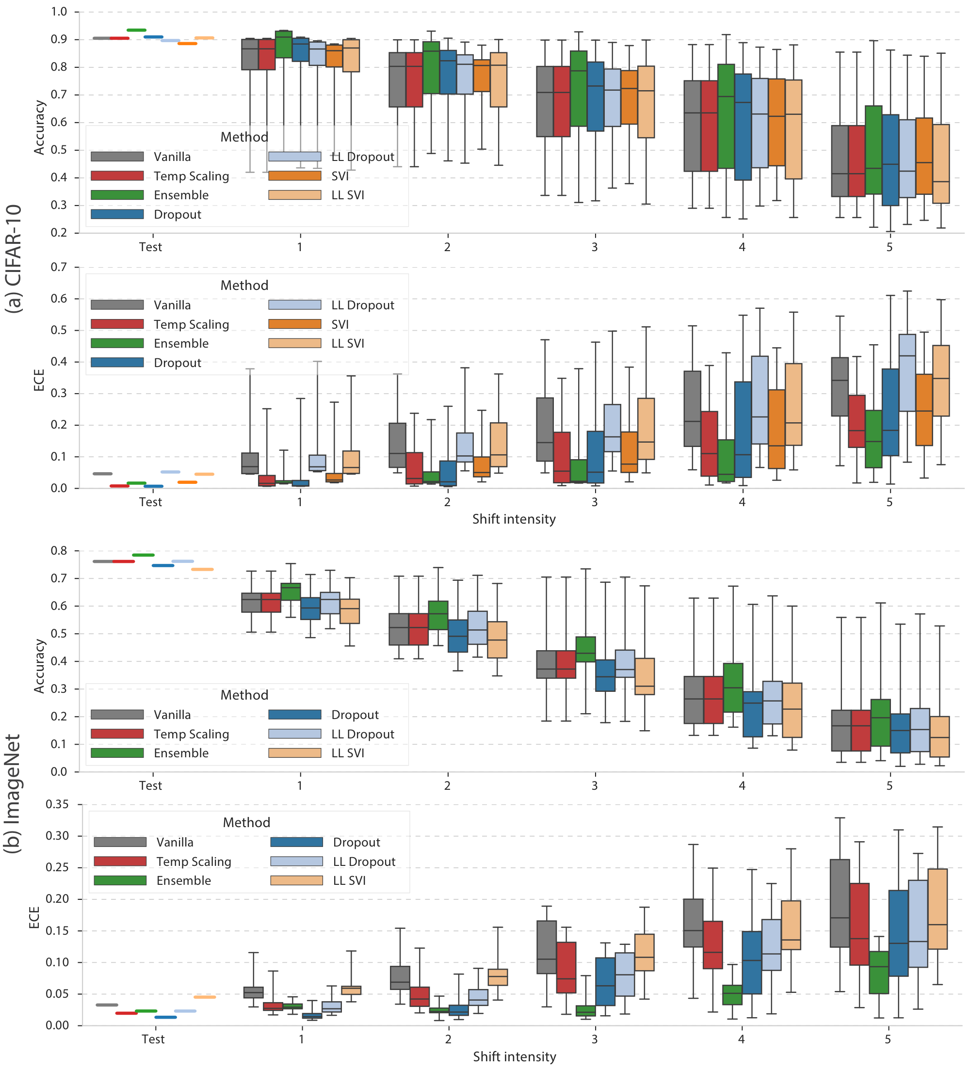
We now study the predictive distributions of residual networks ([47]) trained on two benchmark image datasets, CIFAR-10 ([48]) and ImageNet ([49]), under distributional shift. We use 20-layer and 50-layer ResNets for CIFAR-10 and ImageNet respectively. For shifted data we use 80 different distortions (16 different types with 5 levels of intensity each, see Appendix B for illustrations) introduced by [20]. To evaluate predictions of CIFAR-10 models on entirely OOD data, we use the SVHN dataset ([50]).

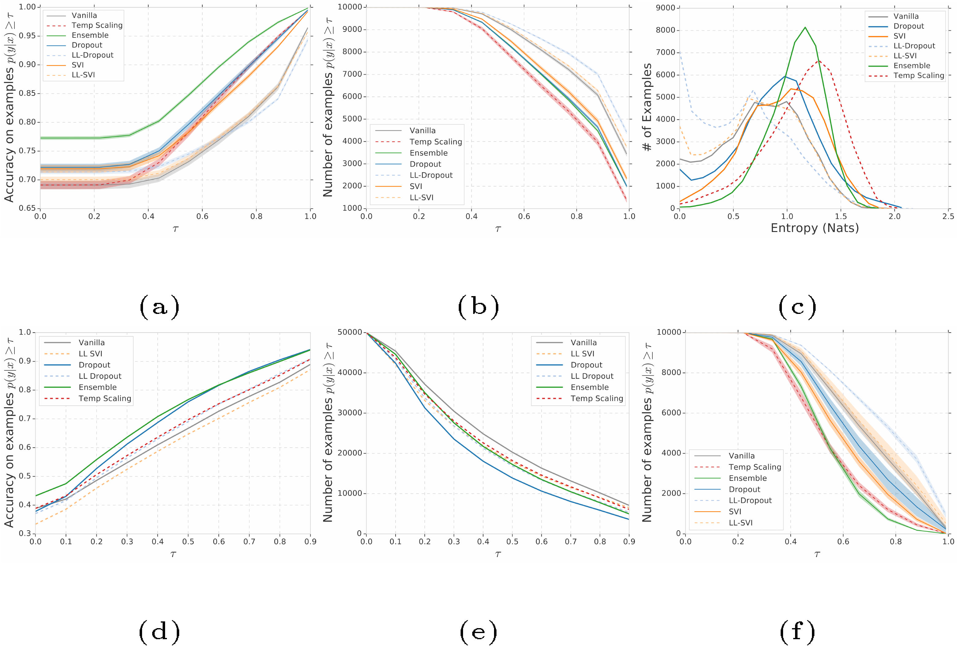
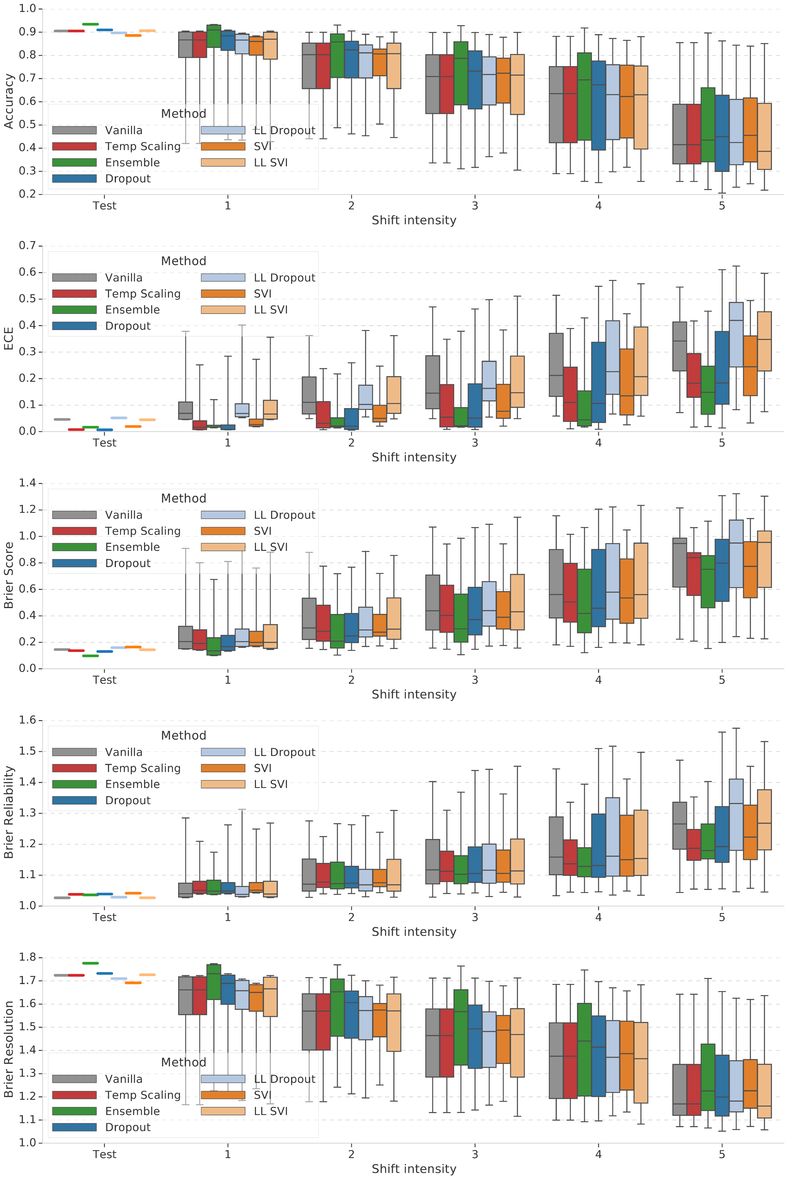
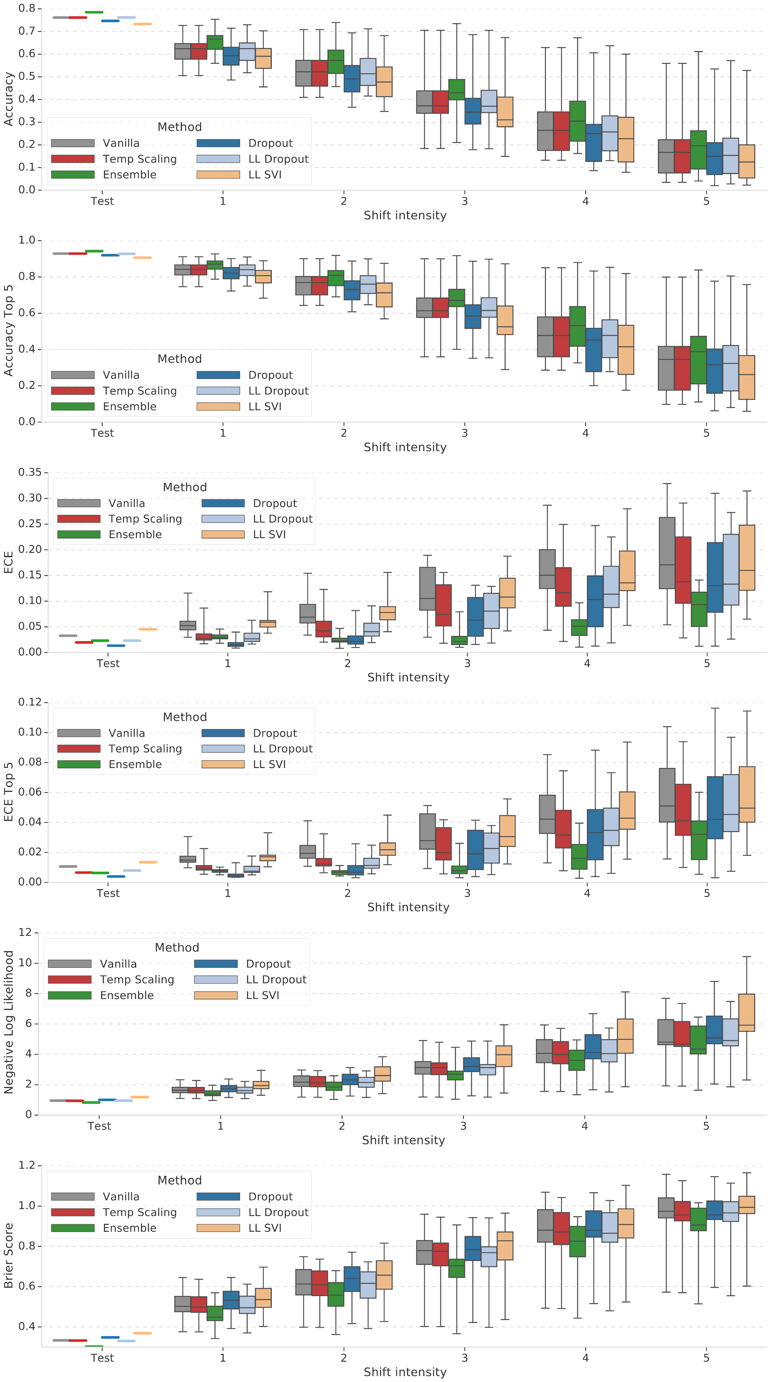
Figure 2 summarizes the accuracy and ECE for CIFAR-10 (top) and ImageNet (bottom) across all 80 combinations of corruptions and intensities from ([20]). Figure 3 inspects the predictive distributions of the models on CIFAR-10 (top) and ImageNet (bottom) for shifted (Gaussian blur) and OOD data. Classifiers on both datasets show poorer accuracy and calibration with increasing shift. Comparing accuracy for different methods, we see that ensembles achieve highest accuracy under distributional shift. Comparing the ECE for different methods, we observe that while the methods achieve comparable low values of ECE for small values of shift, ensembles outperform the other methods for larger values of shift. To test whether this result is due simply to the larger aggregate capacity of the ensemble, we trained models with double the number of filters for the Vanilla and Dropout methods. The higher-capacity models showed no better accuracy or calibration for medium- to high-shift than the corresponding lower-capacity models (see Appendix C). In Figure 19 and Figure 20 we also explore the effect of the number of samples used in dropout, SVI and last layer methods and size of the ensemble, on CIFAR-10. We found that while increasing ensemble size up to 50 did help, most of the gains of ensembling could be achieved with only 5 models. Interestingly, while temperature scaling achieves low ECE for low values of shift, the ECE increases significantly as the shift increases, which indicates that calibration on the i.i.d. validation dataset does not guarantee calibration under distributional shift. (Note that for ImageNet, we found similar trends considering just the top-5 predicted classes, See Figure 13.) Furthermore, the results show that while temperature scaling helps significantly over the vanilla method, ensembles and dropout tend to be better. In Figure 3, we see that ensembles and dropout are more accurate at higher confidence. However, in Figure 3c we see that temperature scaling gives the highest entropy on OOD data. Ensembles consistently have high accuracy but also high entropy on OOD data. We refer to Appendix C for additional results; Figure 12 and Figure 13 report additional metrics on CIFAR-10 and ImageNet, such as Brier score (and its component terms), as well as top-5 error for increasing values of shift.

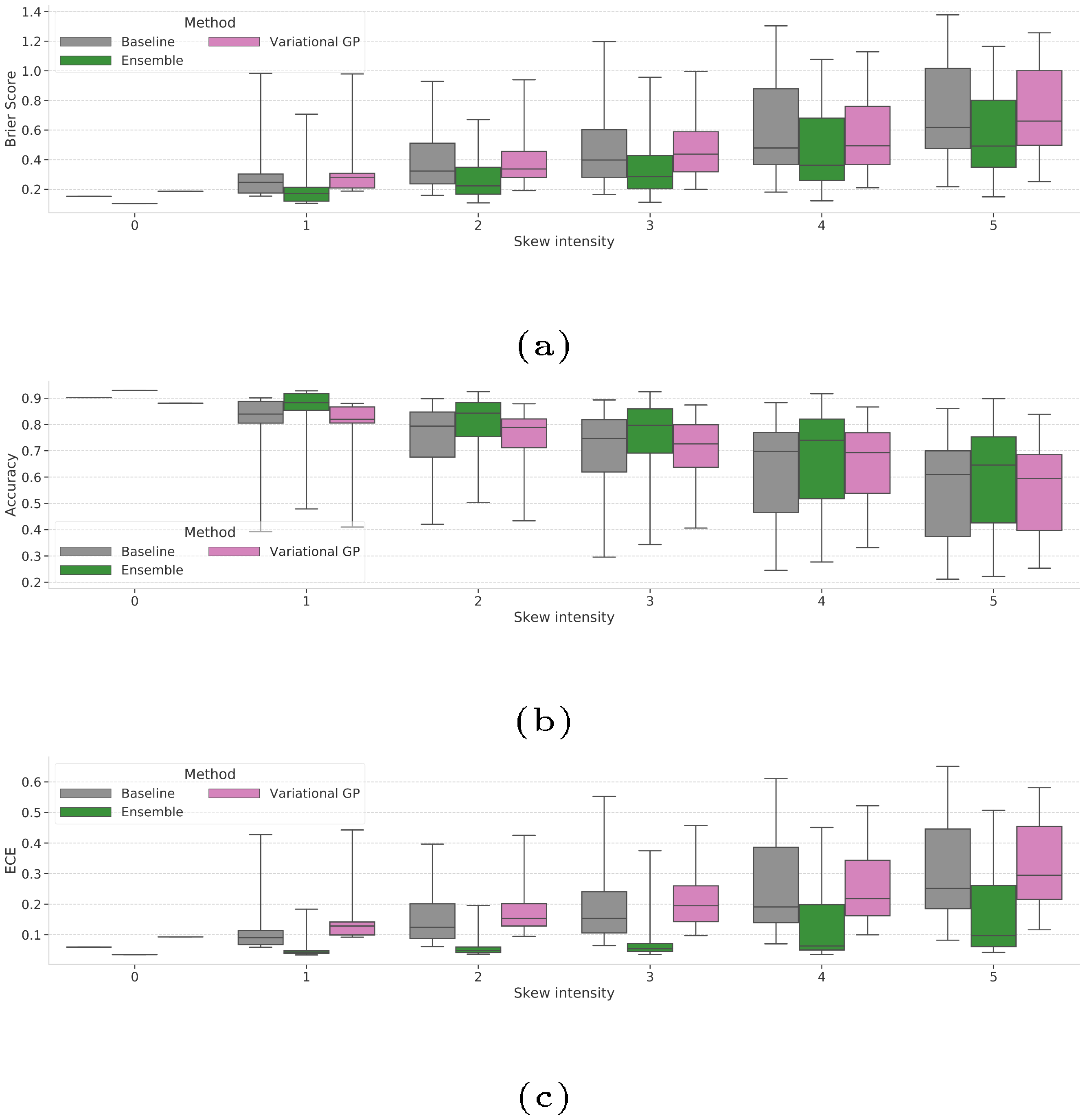
Overall, ensembles consistently perform best across metrics and dropout consistently performed better than temperature scaling and last layer methods. While the relative ordering of methods is consistent on both CIFAR-10 and ImageNet (ensembles perform best), the ordering is quite different from that on MNIST where SVI performs best. Interestingly, LL-SVI and LL-Dropout perform worse than the vanilla method on shifted datasets as well as SVHN. We also evaluate a variational Gaussian process as a last layer method in Appendix E but it did not outperform LL-SVI and LL-Dropout.

4.3 Text Models

Following [32], we train an LSTM ([51]) on the 20newsgroups dataset ([52]) and assess the model's robustness under distributional shift and OOD text. We use the even-numbered classes (10 classes out of 20) as in-distribution and the 10 odd-numbered classes as shifted data. We provide additional details in Appendix A.4.

We look at confidence vs accuracy when the test data consists of a mix of in-distribution and either shifted or completely OOD data, in this case the One Billion Word Benchmark (LM1B) ([53]). Figure 4 (bottom row) shows the results. Ensembles significantly outperform all other methods, and achieve better trade-off between accuracy versus confidence. Surprisingly, LL-Dropout and LL-SVI perform worse than the vanilla method, giving higher confidence incorrect predictions, especially when tested on fully OOD data.

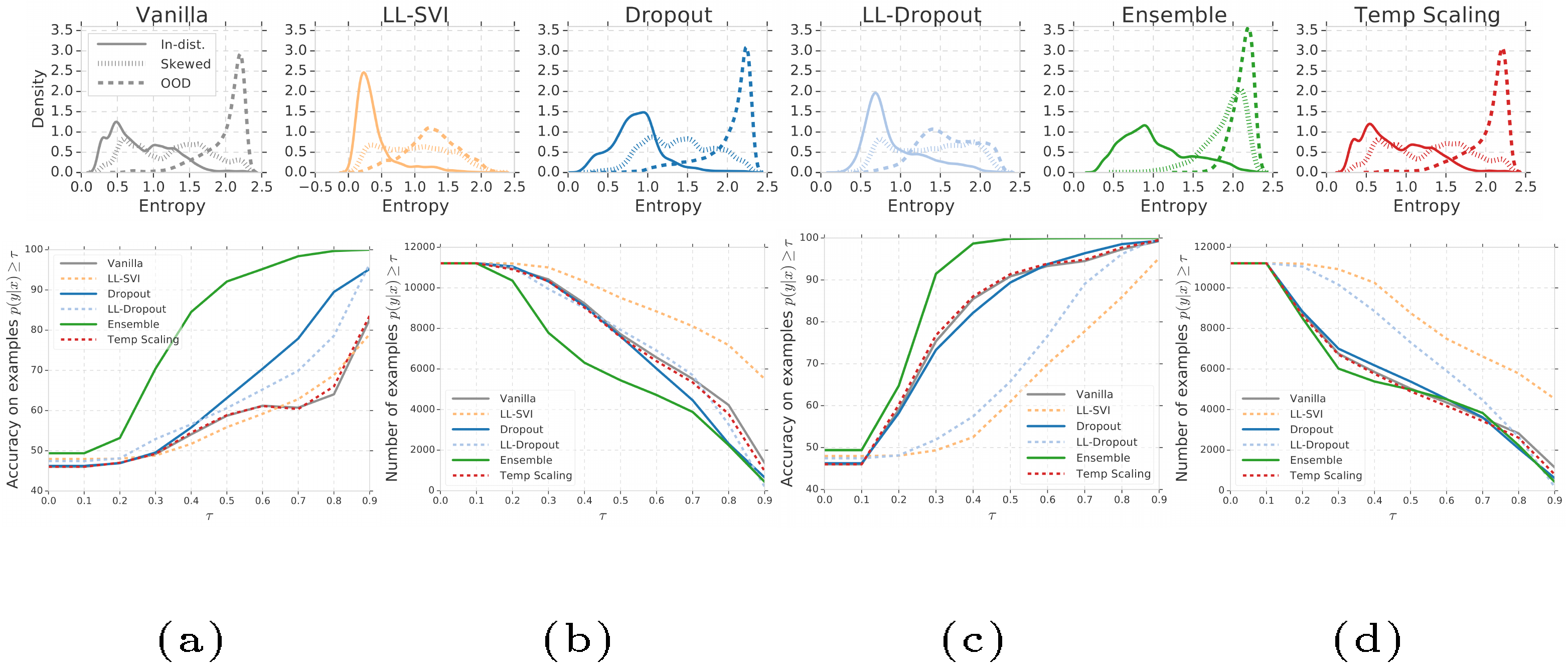
Figure 4 reports histograms of predictive entropy on in-distribution data and compares them to those for the shifted and OOD datasets. This reflects how amenable each method is to abstaining from prediction by applying a threshold on the entropy. As expected, most methods achieve the highest predictive entropy on the completely OOD dataset, followed by the shifted dataset and then the in-distribution test dataset. Only ensembles have consistently higher entropy on the shifted data, which explains why they perform best on the confidence vs accuracy curves in the second row of Figure 4. Compared with the vanilla model, Dropout and LL-SVI have more a distinct separation between in-distribution and shifted or OOD data. While Dropout and LL-Dropout perform similarly on in-distribution, LL-Dropout exhibits less uncertainty than Dropout on shifted and OOD data. Temperature scaling does not appear to increase uncertainty significantly on the shifted data.

4.4 Ad-Click Model with Categorical Features

Finally, we evaluate the performance of different methods on the Criteo Display Advertising Challenge^3 dataset, a binary classification task consisting of 37M examples with 13 numerical and 26 categorical features per example. We introduce shift by reassigning each categorical feature to a random new token with some fixed probability that controls the intensity of shift. This coarsely simulates a type of shift observed in non-stationary categorical features as category tokens appear and disappear over time, for example due to hash collisions. The model consists of a 3-hidden-layer multi-layer-perceptron (MLP) with hashed and embedded categorical features and achieves a negative log-likelihood of approximately 0.5 (contest winners achieved 0.44). Due to class imbalance ($\sim25%$ of examples are positive), we report AUC instead of classification accuracy.

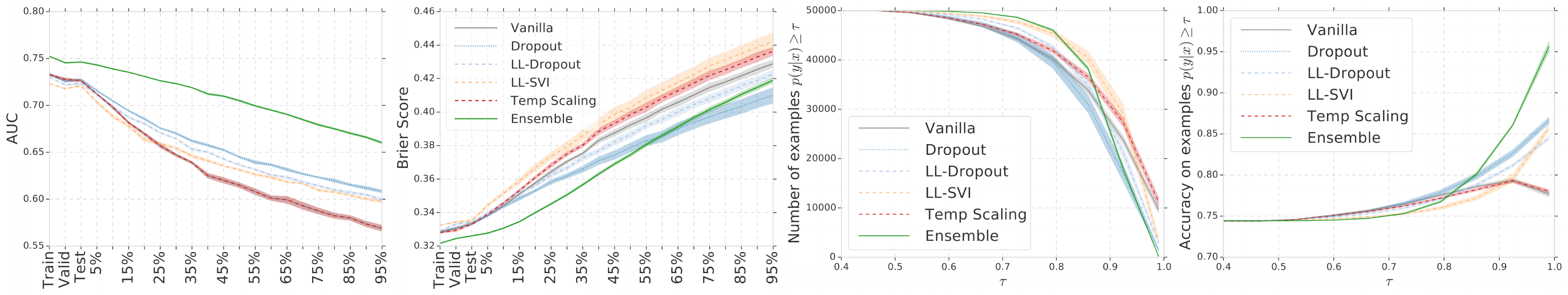
Results from these experiments are depicted in Figure 5. (Figure 18 in Appendix C shows additional results including ECE and Brier score decomposition.) We observe that ensembles are superior in terms of both AUC and Brier score for most of the values of shift, with the performance gap between ensembles and other methods generally increasing as the shift increases. Both Dropout model variants yielded improved AUC on shifted data, and Dropout surpassed ensembles in Brier score at shift-randomization values above 60%. SVI proved challenging to train, and the resulting model uniformly performed poorly; LL-SVI fared better but generally did not improve upon the vanilla model. Strikingly, temperature scaling has a worse Brier score than Vanilla indicating that post-hoc calibration on the validation set actually harms calibration under dataset shift.

5. Takeaways and Recommendations

Section Summary: This study evaluated various ways to measure predictive uncertainty when data changes, finding that uncertainty quality drops sharply with increasing data shifts across different data types and models, even if methods work well on standard data. Deep ensembles stood out as the top performer, handling shifts robustly with small group sizes, while other approaches like post-hoc calibration faltered on larger shifts and methods like stochastic variational inference showed promise only on smaller datasets. The results held up on a real-world genomics task, but all methods have room for improvement, and future work should tackle their high computational costs to make them more practical.

We presented a large-scale evaluation of different methods for quantifying predictive uncertainty under dataset shift, across different data modalities and architectures. Our take-home messages are the following:

• Along with accuracy, the quality of uncertainty consistently degrades with increasing dataset shift regardless of method.
• Better calibration and accuracy on the i.i.d. test dataset does not usually translate to better calibration under dataset shift (shifted versions as well as completely different OOD data).
• Post-hoc calibration (on i.i.d validation) with temperature scaling leads to well-calibrated uncertainty on the i.i.d. test set and small values of shift, but is significantly outperformed by methods that take epistemic uncertainty into account as the shift increases.
• Last layer Dropout exhibits less uncertainty on shifted and OOD datasets than Dropout.
• SVI is very promising on MNIST/CIFAR but it is difficult to get to work on larger datasets such as ImageNet and other architectures such as LSTMs.
• The relative ordering of methods is mostly consistent (except for MNIST) across our experiments. The relative ordering of methods on MNIST is not reflective of their ordering on other datasets.
• Deep ensembles seem to perform the best across most metrics and be more robust to dataset shift. We found that relatively small ensemble size (e.g. $M=5$) may be sufficient (Appendix D).
• We also compared the set of methods on a real-world challenging genomics problem from [54]. Our observations were consistent with the other experiments in the paper. Deep ensembles performed best, but there remains significant room for improvement, as with the other experiments in the paper. See Appendix F for details.

We hope that this benchmark is useful to the community and inspires more research on uncertainty under dataset shift, which seems challenging for existing methods. While we focused only on the quality of predictive uncertainty, applications may also need to consider computational and memory costs of the methods; Table 1 in Appendix A.9 discusses these costs, and the best performing methods tend to be more expensive. Reducing the computational and memory costs, while retaining the same performance under dataset shift, would also be a key research challenge.

Acknowledgements

We thank Alexander D'Amour, Jakub Świątkowski and our reviewers for helpful feedback that improved the manuscript.

Appendix

Section Summary: The appendix outlines the technical details of the models and training processes used in the study across various datasets. For image-based datasets like MNIST, CIFAR-10, and ImageNet, it describes architectures such as LeNet and ResNet, along with training setups involving optimizers like Adam or SGD, data augmentations like random flips and crops, and hyperparameter tuning for things like learning rates and dropout. It also explains text preprocessing for 20 Newsgroups using LSTM models and feature encoding for the Criteo dataset with multilayer perceptrons, plus specifics on uncertainty methods like ensembles, stochastic sampling, and variational inference.

Can You Trust Your Model's Uncertainty? Evaluating Predictive Uncertainty Under Dataset Shift: Appendix

A. Model Details

A.1 MNIST

We evaluated both LeNet and a fully-connected neural network (MLP) under shift on MNIST. We observed similar trends across metrics for both models, so we report results only for LeNet in Figure 1. LeNet and MLP were trained for 20 epochs using the Adam optimizer ([55]) and used ReLU activation functions. For stochastic methods, we averaged 300 sample predictions to yield a predictive distribution, and the ensemble model used 10 instances trained from independent random initializations. The MLP architecture consists of two hidden layers of 200 units each with dropout applied before every dense layer. The LeNet architecture ([45]) applies two convolutional layers 3x3 kernels of 32 and 64 filters respectively) followed by two fully-connected layers with one hidden layer of 128 activations; dropout was applied before each fully-connected layer. We employed hyperparameter tuning (See Appendix A.8) to select the training batch size, learning rate, and dropout rate.

A.2 CIFAR-10

Our CIFAR model used the ResNet-20 V1 architecture with ReLU activations. Model parameters were trained for 200 epochs using the Adam optimizer and employed a learning rate schedule that multiplied an initial learning rate by 0.1, 0.01, 0.001, and 0.0005 at steps 80, 120, 160, and 180 respectively. Training inputs were randomly distorted using horizontal flips and random crops preceded by 4-pixel padding as described in ([47]). For relevant methods, dropout was applied before each convolutional and dense layer (excluding the raw inputs), and stochastic methods sampled 128 predictions per sample. Hyperparameter tuning was used to select the initial learning rate, training batch size, and the dropout rate.

A.3 ImageNet 2012

Our ImageNet model used the ResNet-50 V1 architecture with ReLU activations and was trained for 90 epochs using SGD with Nesterov momentum. The learning rate schedule linearly ramps up to a base rate in 5 epochs and scales down by a factor of 10 at each of epochs 30, 60, and 80. As with the CIFAR-10 model, stochastic methods used a sample-size of 128. Training images were distorted with random horizontal flips and random crops.

A.4 20 Newsgroups

We use a pre-processing strategy similar to the one proposed by [32] for 20 Newsgroups. We build a vocabulary of size 30, 000 words and words are indexed based on the word frequencies. The rare words are encoded as unknown words. We fix the length of each text input by setting a limit of 250 words, and those longer than 250 words are truncated, and those shorter than 250 words are padded with zeros. Text in even-numbered classes are used as in-distribution inputs, and text from the odd-numbered of classes are used shifted OOD inputs. A dataset with the same number of randomly selected text inputs from the LM1B dataset ([53]) is used as completely different OOD dataset. The classifier is trained and evaluated only using the text from the even-numbered in-distribution classes in the training dataset. The final test results are evaluated based on in-distribution test dataset, shift OOD test dataset, and LM1B dataset.

The vanilla model uses a one-layer LSTM model of size 32 and a dense layer to predict the 10 class probabilities based on word embedding of size 128. A dropout rate of 0.1 is applied to both the LSTM layer and the dense layer for the Dropout model. The LL-SVI model replaces the last dense layer with a Bayesian layer, the ensemble model aggregates 10 vanilla models, and stochastic methods sample 5 predictions per example. The vanilla model accuracy for in-distribution test data is 0.955.

A.5 Criteo

Each categorical feature $x_k$ from the Criteo dataset was encoded by hashing the string token into a fixed number of buckets $N_k$ and either encoding the hash-bin as a one-hot vector if $N_k < 110$ or embedding each bucket as a $d_k$ dimensional vector otherwise. This dense feature vector, concatenated with 13 numerical features, feeds into a batch-norm layer followed by a 3-hidden-layer MLP. Each model was trained for one epoch using the Adam optimizer with a non-decaying learning rate.

Values of $N_k$ and $d_k$ were tuned to maximize log-likelihood for a vanilla model, and the resulting architectural parameters were applied to all methods. This tuning yielded hidden-layers of size 2572, 1454, and 1596, and hash-bucket counts and embedding dimensions of sizes listed below:

$ \begin{align*} N_k = [&1373, 2148, 4847, 9781, 396, 28, 3591, 2798, 14, 7403, 2511, 5598, 9501, \ &46, 4753, 4056, 23, 3828, 5856, 12, 4226, 23, 61, 3098, 494, 5087] \ d_k = [&3, 9, 29, 11, 17, 0, 14, 4, 0, 12, 19, 24, 29, 0, 13, 25, 0, 8, 29, 0, 22, 0, 0, 31, 0, 29] \ \end{align*} $

Learning rate, batch size, and dropout rate were further tuned for each method. Stochastic methods used 128 prediction samples per example.

A.6 Stochastic Variational Inference Details

For MNIST we used Flipout ([36]), where we replaced each dense layer and convolutional layer with mean-field variational dense and convolutional Flipout layers respectively. Variational inference for deep ResNets ([47]) is non-trivial, so for CIFAR we replaced a single linear layer per residual branch with a Flipout layer, removed batch normalization, added Selu non-linearities ([56]), empirical Bayes for the prior standard deviations as in [57] and careful tuning of the initialization via Bayesian optimization.

A.7 Variational Gaussian Process Details

For the experiments where Gaussian Processes were compared, we used Variational Gaussian Processes to fit the model logits as in [31]. These were then passed through a Categorical distribution and numerically integrated over using Gauss-Hermite quadrature. Each class was treated as a separate Gaussian Process, with 100 inducing points used for each class. The inducing points were initialized with model outputs on random dataset examples for CIFAR, and with Gaussian noise for MNIST. Uniform noise inducing point initialization was also tested but there was negligible difference between the three methods. All zero inducing points initializations numerically failed early on in training. Exponentiated quadratic plus linear kernels were used for all experiments. 250 samples were drawn from the logit distribution during training time to get a better estimate of the ELBO to backpropagate through. 250 logit samples were drawn at test time. $10^{-5} * I$ was added to the diagonal of the covariance matrix to ensure positive definiteness.

We used 100 trials of random hyperparamter settings, selecting the configuration with the best final validation accuracy. The learning rate was tuned in $\lbrack 10^{-4}, 1.0\rbrack$ on a log scale; the initial kernel amplitude in $\lbrack -2.0, 2.0\rbrack$; the initial kernel length scale in $\lbrack -2.0, 2.0\rbrack$; the variational distribution covariance was initialized to $s * I$ where $s$ was tuned in $\lbrack 0.1, 2.0\rbrack$; $1 - \beta_1$ in Adam was tuned on $\lbrack 10^{-2}, 0.15\rbrack$ on a log scale.

The Adam optimizer with a batch size of 512 was used, training for the same number of epochs as other methods. The same learning rate schedule was as other methods for the model and kernel parameters, but the learning rate for the variational parameters also included a 5 epoch warmup in order to help with numerical stability.

A.8 Hyperparameter Tuning

Hyperparameters were optimized through Bayesian optimization using Google Vizier ([44]). We maximized the log-likelihood on a validation set that was held out from training (10K examples for MNIST and CIFAR-10, 125K examples for ImageNet). We optimized log-likelihood rather than accuracy since the former is a proper scoring rule.

A.9 Computational and Memory Complexity of Different methods

In addition to performance, applications may also need to consider computational and memory costs; Table 1 discusses them for each method.

: Table 1: Computational and memory costs for evaluated methods. Notation: $m$ represents flops or storage for the full model, $d$ represents flops or storage for the last layer, $k$ denotes replications, $z$ the number of inducing points for Gaussian Processes, $n$ denotes number of evaluated points, and $v$ denotes the validation set size. Serving/training compute is identical except that $v=0$ for serving. Implicit in this table is a memory/compute tradeoff for sampling. Sampled weights/masks need not be stored explicitly via PRNG seed reuse; we assume the computational cost of sampling is zero.

Method	Compute/ $n$	Storage
Vanilla	$m$	$m$
Temp Scaling	$m + v m/n$	$m$
LL-Dropout	$m + d(k-1)$	$m$
LL-SVI	$m + d(k-1)$	$m + d$
SVI	$m k$	$2 m $
Dropout	$ m k $	$ m $
Gaussian Process	$ m + z^3 $	$ m + z^2 $
Ensemble	$ m k $	$ m k$

B. Shifted Images

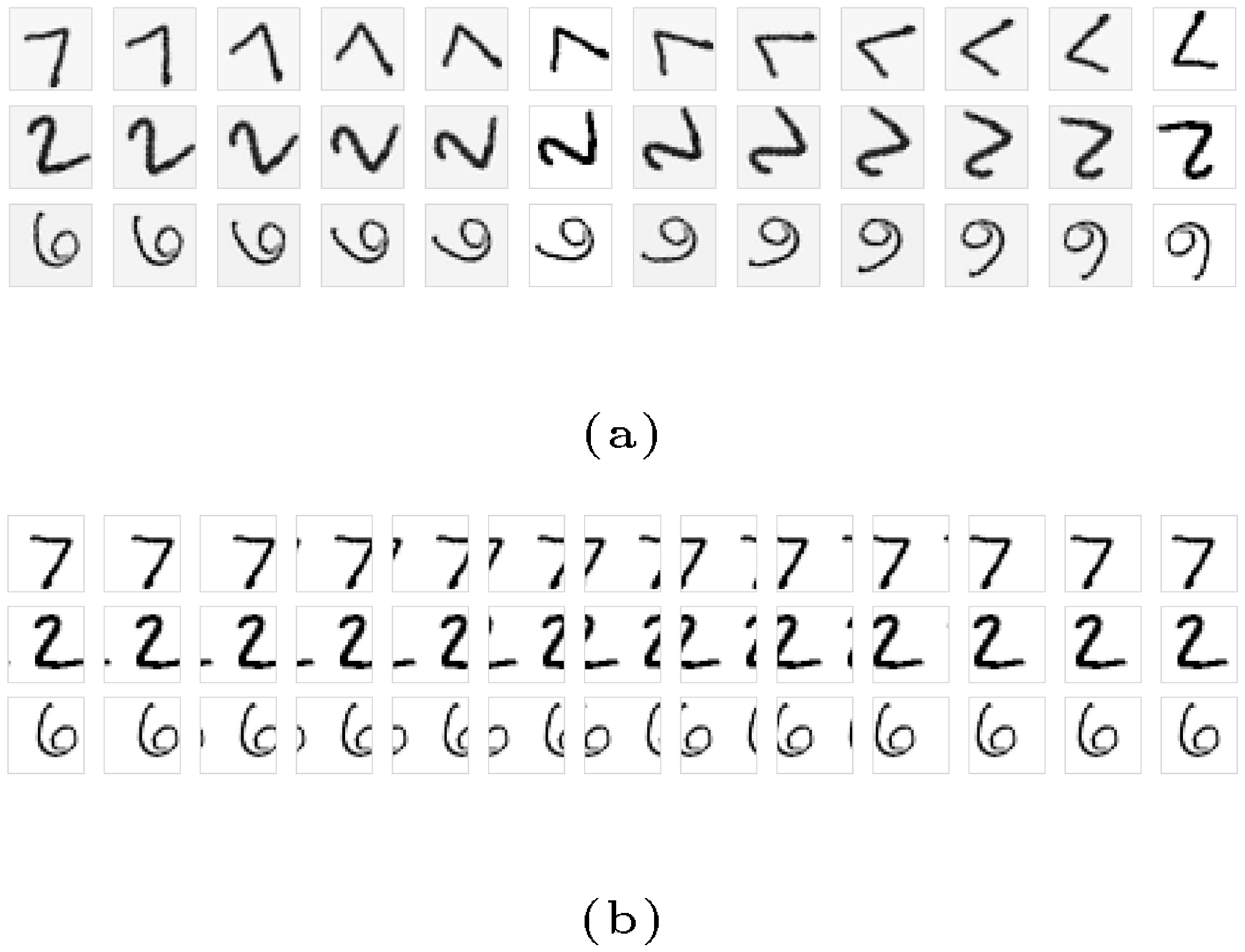
We distorted MNIST images using rotations with spline filter interpolation and cyclic translations as depicted in Figure 6.

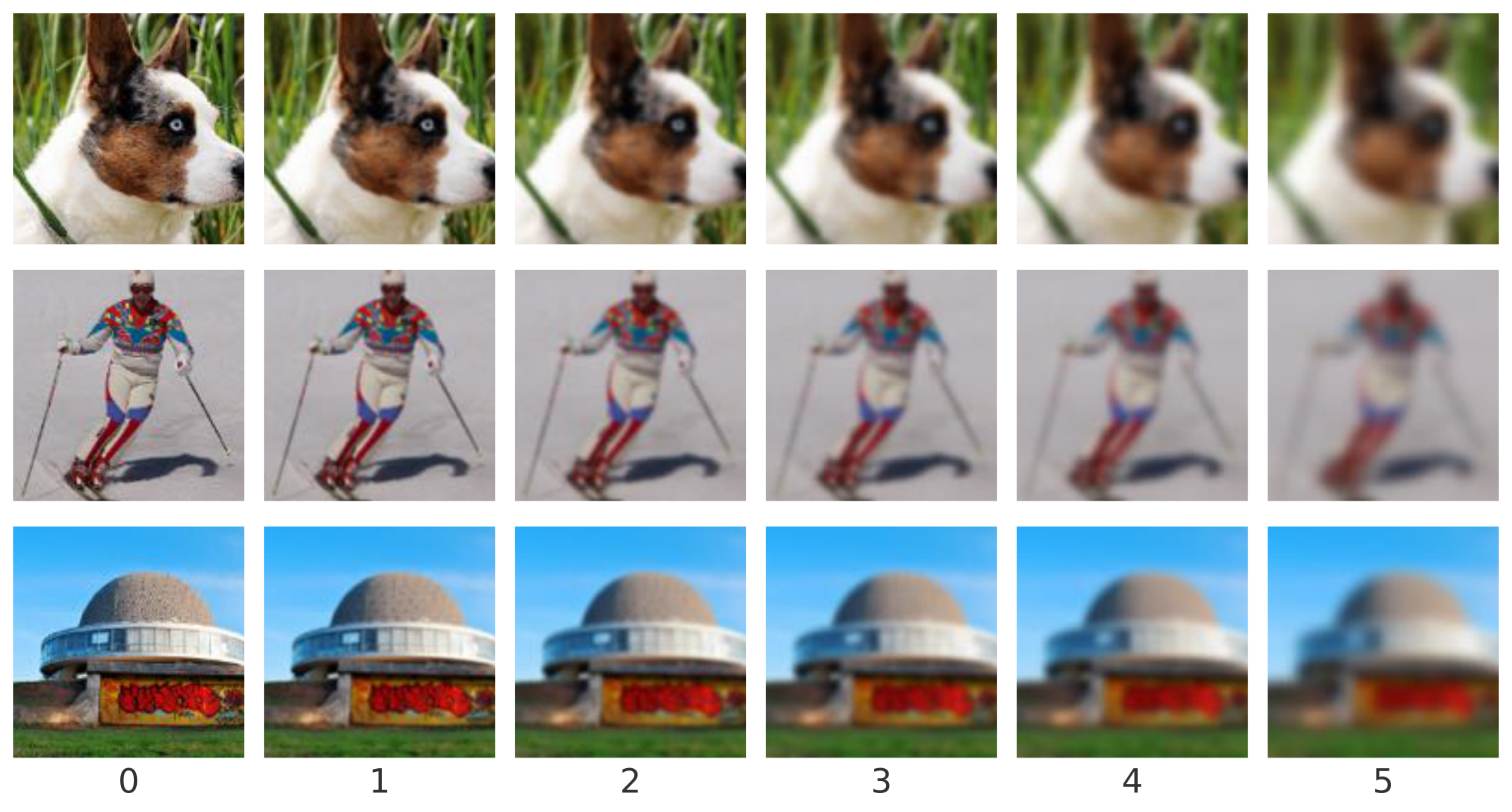
For the corrupted ImageNet dataset, we used ImageNet-C ([20]). Figure 7 shows examples of ImageNet-C images at varying corruption intensities. Figure 8 shows ImageNet-C images with the 16 corruptions analyzed in this paper, at intensity 3 (on a scale of 1 to 5).

:::: {cols="2"}

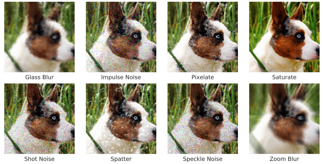
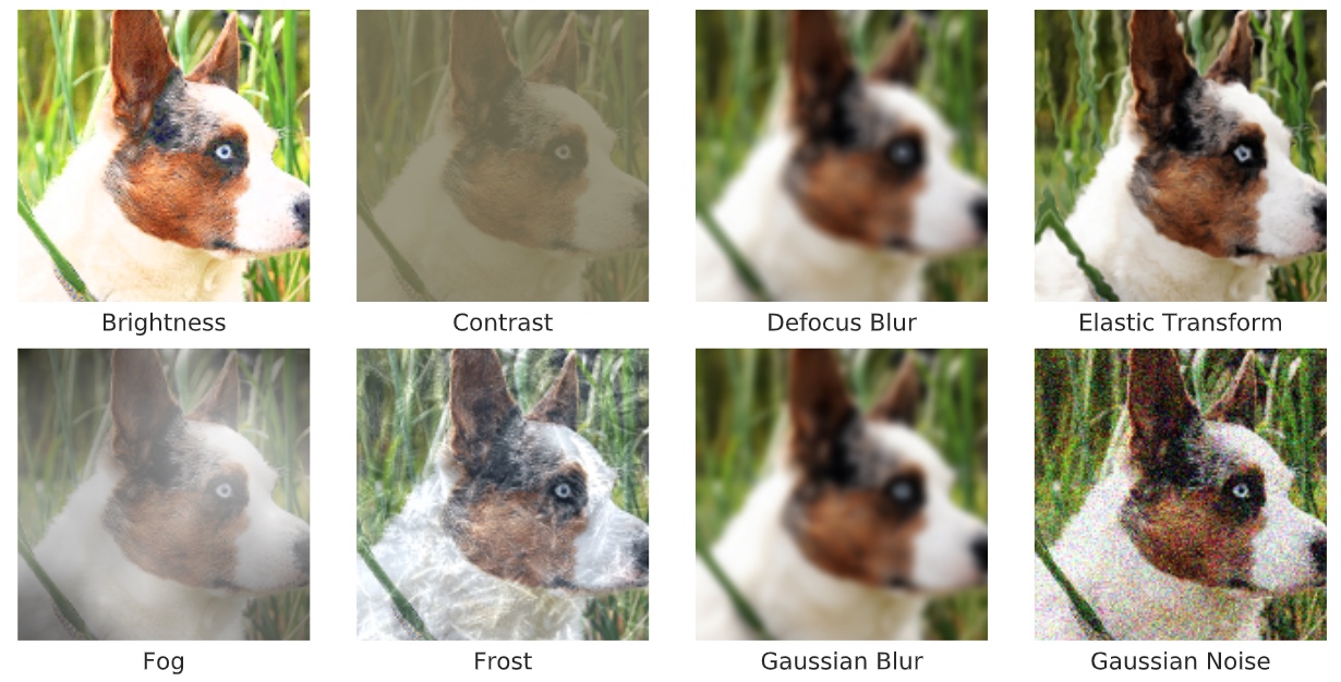
Figure 8: Examples of 16 corruption types in ImageNet-C images, at corruption intensity 3 (on a scale from 1–5). The same corruptions were applied to CIFAR-10. Figure 2 and Appendix C show boxplots for each uncertainty method and corruption intensity, spanning all corruption types. ::::

C. Evaluating uncertainty under distributional shift: Additional Results

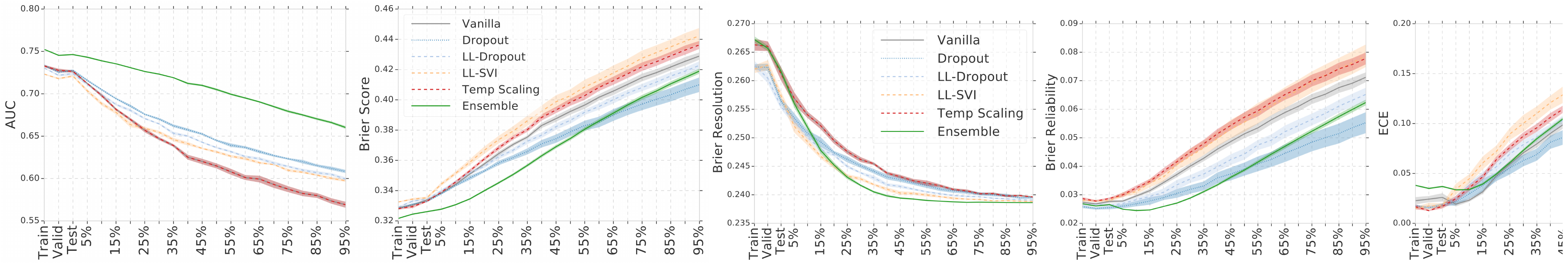
Figure 12, Figure 13 and Figure 18 show comprehensive results on CIFAR-10, ImageNet and Criteo respectively across various metrics including Brier score, along with the components of the Brier score : reliability (lower means better calibration) and resolution (higher values indicate better predictive quality). Ensembles and dropout outperform all other methods across corruptions, while LL SVI shows no improvement over the baseline model. Figure 14 shows accuracy and ECE for models with double the number of ResNet filters; the higher-capacity models are not better calibrated than their lower-capacity counterparts, suggesting that the good calibration performance of ensembles is not due simply to higher capacity.

:::: {cols="1"}

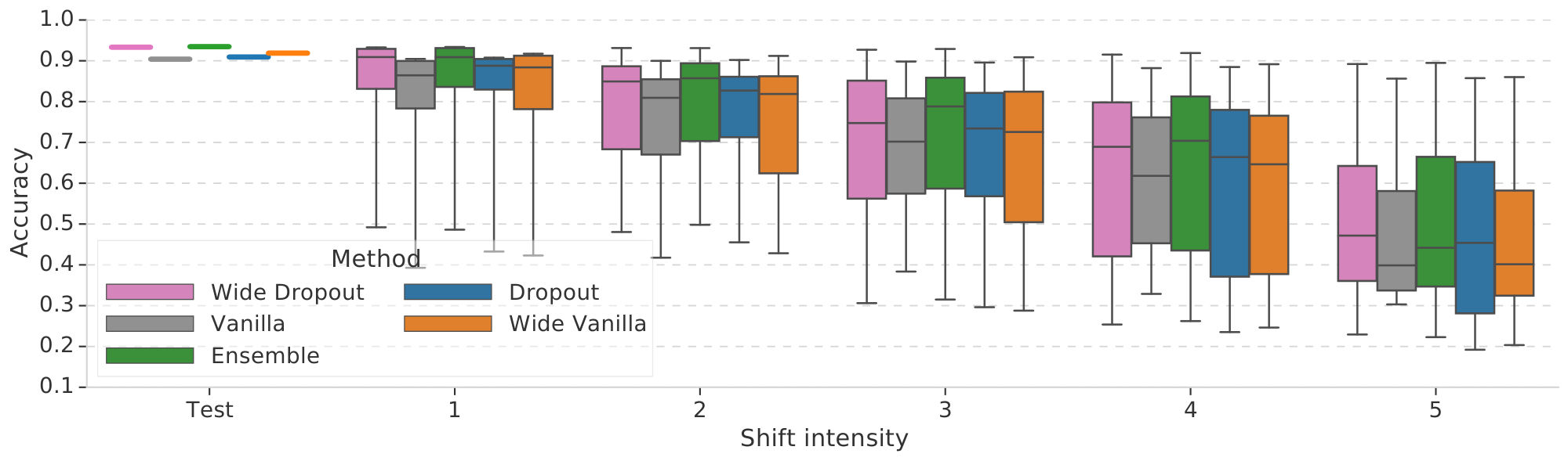
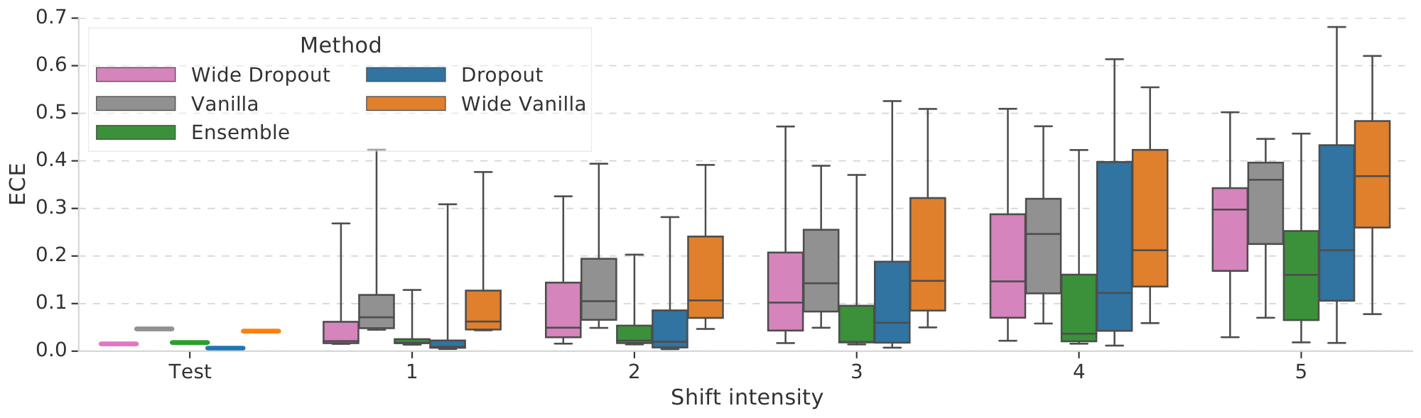
Figure 14: Boxplots facilitating comparison of results for higher-capacity models ('Wide Vanilla' and 'Wide Dropout') with their lower-capacity counterparts on CIFAR. Each box shows the quartiles summarizing the results across all types of shift while the error bars indicate the min and max across different shift types. ::::

D. Effect of the number of samples on the quality of uncertainty

Figure 19 shows the effect of the number of sample sizes used by Dropout, SVI (and last-layer variants) on the quality of predictive uncertainty, as measured by the Brier score. Increasing the number of samples has little effect on last-layer variants, whereas increasing the number of samples improves the performance for SVI and Dropout, with diminishing returns beyond size 5.

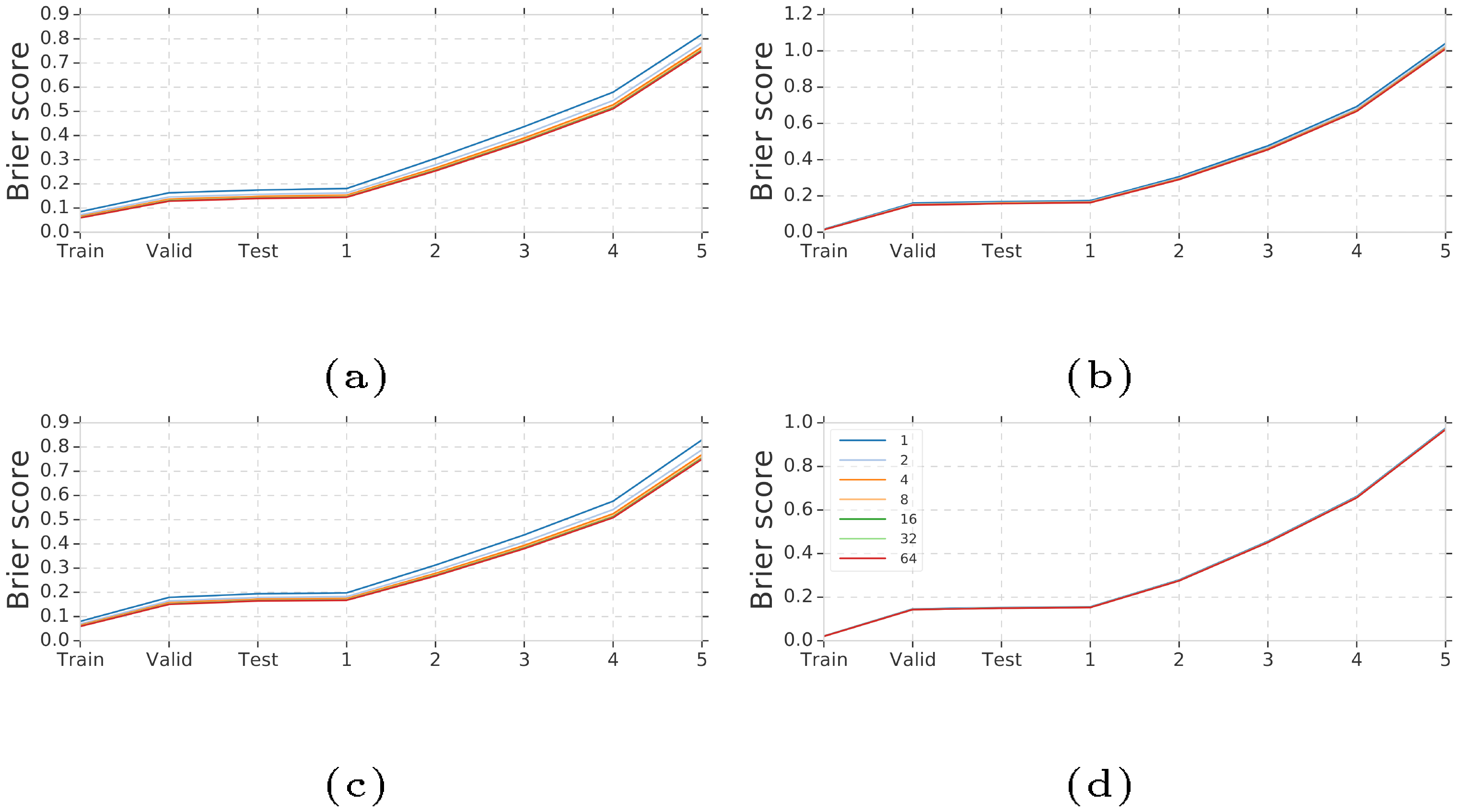
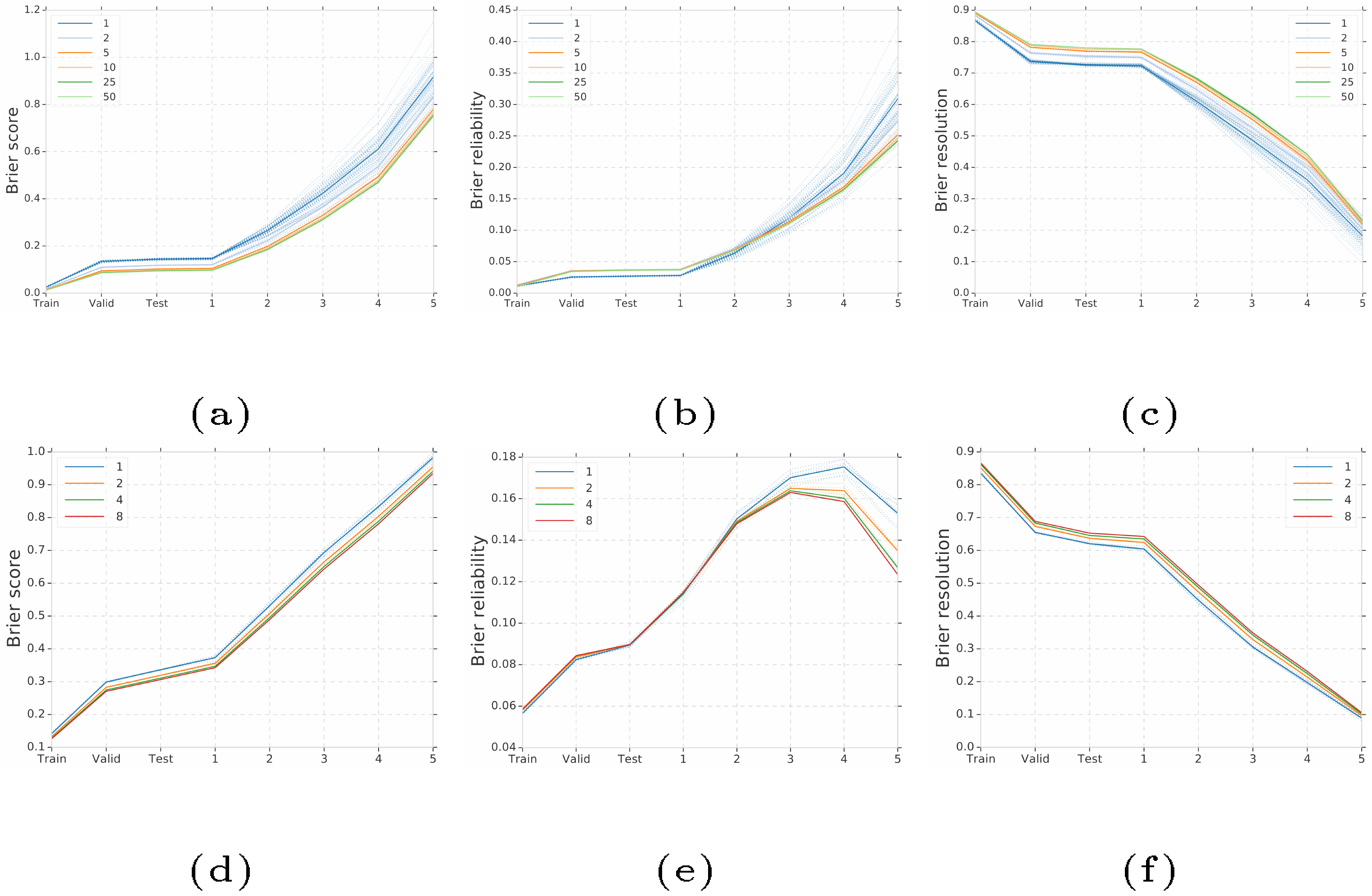
Figure 20 shows the effect of ensemble size on CIFAR-10 (top) and ImageNet (bottom). Similar to SVI and Dropout, we see that increasing the number of models in the ensemble improves performance with diminishing returns beyond size 5. As mentioned earlier, the Brier score can be further decomposed into $\mathrm{BS} = \mathrm{calibration} + \mathrm{refinement} = \mathrm{reliability} + \mathrm{uncertainty} - \mathrm{resolution}$ where $\mathrm{reliability} \downarrow$ measures calibration as the average violation of long-term true label frequencies, and $\mathrm{refinement}=\mathrm{uncertainty} - \mathrm{resolution}$, where $\mathrm{uncertainty}$ is the marginal uncertainty over labels (independent of predictions) and $\mathrm{resolution} \uparrow$ measures the deviation of individual predictions from the marginal.

E. Variational Gaussian Process Results

F. OOD detection for genomic sequences

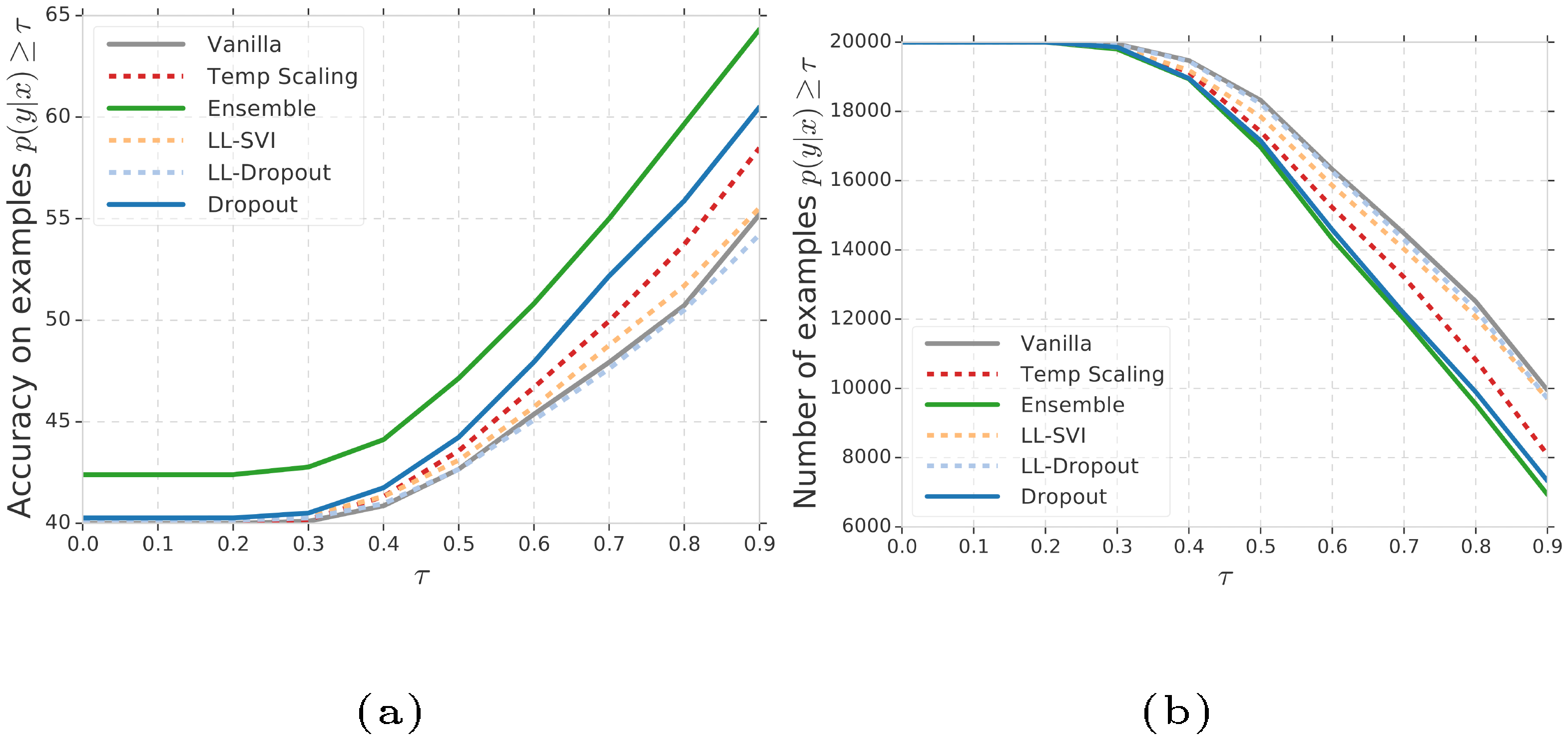
We studied the set of methods for detecting OOD genomic sequence, as a challenging realistic problem for OOD detection proposed by [54]. Classifiers are trained on 10 in-distribution bacteria classes, and tested for OOD detection of 60 OOD bacteria classes. The model architecture is the same as that in [54]: a convolutional neural networks with 1000 filters of length 20, followed by a global max pooling layer, a dense layer of 1000 units, and a last dense layer that outputs class prediction logits. For the dropout method, we add a dropout layer each after the max pooling layer and the dense layer respectively. For the LL-Dropout method, only a dropout layer after the dense layer is added. We use the dropout rate of 0.2. For the LL-SVI method, we replace the last dense layer with a stochastic variational inference dense layer. The classification accuracy for in-distribution is around 0.8 for the various types of classifiers.

Figure 22 shows the confidence vs (a) accuracy and (b) count when the test data consists of a mix of in-distribution and OOD data. Ensembles significantly outperform all other methods, and achieve better trade-off between accuracy versus confidence. Dropout performs better than Temp Scaling, and they both perform better than LL-Dropout, LL-SVI, and the Vanilla method. Note that the accuracy on examples $p(y| {\bm{x}})\geq0.9$ for the best method is still below 65%, suggesting that this realistic genomic sequences dataset is a challenging problem to benchmark future methods.

G. Tables of Metrics

The tables below report quartiles of Brier score, negative log-likelihood, and ECE for each model and dataset where quartiles are computed over all corrupted variants of the dataset.

G.1 CIFAR-10

\begin{tabular}{l|rrrrrrr}
Method & Vanilla & Temp. Scaling & Ensembles & Dropout & LL-Dropout & SVI & LL-SVI \\
\midrule
Brier Score (25th) & 0.243 & 0.227 & 0.165 & 0.215 & 0.259 & 0.250 & 0.246 \\
Brier Score (50th) & 0.425 & 0.392 & 0.299 & 0.349 & 0.416 & 0.363 & 0.431 \\
Brier Score (75th) & 0.747 & 0.670 & 0.572 & 0.633 & 0.728 & 0.604 & 0.732 \\
\midrule
NLL (25th) & 2.356 & 1.685 & 1.543 & 1.684 & 2.275 & 1.628 & 2.352 \\
NLL (50th) & 1.120 & 0.871 & 0.653 & 0.771 & 1.086 & 0.823 & 1.158 \\
NLL (75th) & 0.578 & 0.473 & 0.342 & 0.446 & 0.626 & 0.533 & 0.591 \\
\midrule
ECE (25th) & 0.057 & 0.022 & 0.031 & 0.021 & 0.069 & 0.029 & 0.058 \\
ECE (50th) & 0.127 & 0.049 & 0.037 & 0.034 & 0.136 & 0.064 & 0.135 \\
ECE (75th) & 0.288 & 0.180 & 0.110 & 0.174 & 0.292 & 0.187 & 0.275 \\
\end{tabular}

G.2 ImageNet

\begin{tabular}{l|rrrrrr}
Method & Vanilla & Temp. Scaling & Ensembles & Dropout & LL-Dropout & LL-SVI \\
\midrule
Brier Score (25th) & 0.553 & 0.551 & 0.503 & 0.577 & 0.550 & 0.590 \\
Brier Score (50th) & 0.733 & 0.726 & 0.667 & 0.754 & 0.723 & 0.766 \\
Brier Score (75th) & 0.914 & 0.899 & 0.835 & 0.922 & 0.896 & 0.938 \\
\midrule
NLL (25th) & 1.859 & 1.848 & 1.621 & 1.957 & 1.830 & 2.218 \\
NLL (50th) & 2.912 & 2.837 & 2.446 & 3.046 & 2.858 & 3.504 \\
NLL (75th) & 4.305 & 4.186 & 3.661 & 4.567 & 4.208 & 5.199 \\
\midrule
ECE (25th) & 0.057 & 0.031 & 0.022 & 0.017 & 0.034 & 0.065 \\
ECE (50th) & 0.102 & 0.072 & 0.032 & 0.043 & 0.071 & 0.106 \\
ECE (75th) & 0.164 & 0.129 & 0.053 & 0.109 & 0.123 & 0.148 \\
\end{tabular}

G.3 Criteo

\begin{tabular}{l|rrrrrrr}
Method & Vanilla & Temp. Scaling & Ensembles & Dropout & LL-Dropout & SVI & LL-SVI \\
\midrule
Brier Score (25th) & 0.353 & 0.355 & 0.336 & 0.350 & 0.353 & 0.512 & 0.361 \\
Brier Score (50th) & 0.385 & 0.391 & 0.366 & 0.373 & 0.379 & 0.512 & 0.396 \\
Brier Score (75th) & 0.409 & 0.416 & 0.395 & 0.393 & 0.403 & 0.512 & 0.421 \\
\midrule
NLL (25th) & 0.581 & 0.594 & 0.508 & 0.532 & 0.542 & 7.479 & 0.554 \\
NLL (50th) & 0.788 & 0.829 & 0.552 & 0.577 & 0.600 & 7.479 & 0.633 \\
NLL (75th) & 0.986 & 1.047 & 0.608 & 0.624 & 0.664 & 7.479 & 0.711 \\
\midrule
ECE (25th) & 0.041 & 0.055 & 0.044 & 0.043 & 0.052 & 0.254 & 0.066 \\
ECE (50th) & 0.097 & 0.113 & 0.100 & 0.085 & 0.100 & 0.254 & 0.127 \\
ECE (75th) & 0.135 & 0.149 & 0.141 & 0.116 & 0.136 & 0.254 & 0.162 \\
\end{tabular}

References

[1] Esteva, A., Kuprel, B., Novoa, R. A., Ko, J., Swetter, S. M., Blau, H. M., and Thrun, S. Dermatologist-level classification of skin cancer with deep neural networks. Nature, 542, 1 2017.

[2] Bojarski, M., Testa, D. D., Dworakowski, D., Firner, B., Flepp, B., Goyal, P., Jackel, L. D., Monfort, M., Muller, U., Zhang, J., Zhang, X., Zhao, J., and Zieba, K. End to end learning for self-driving cars. arXiv preprint arXiv:1604.07316, 2016.

[3] Amodei, D., Olah, C., Steinhardt, J., Christiano, P., Schulman, J., and Mané, D. Concrete problems in AI safety. arXiv preprint arXiv:1606.06565, 2016.

[4] MacKay, D. J. and Gibbs, M. N. Density Networks. Statistics and Neural Networks: Advances at the Interface, 1999.

[5] Kendall, A. and Gal, Y. What uncertainties do we need in Bayesian deep learning for computer vision? In NeurIPS, 2017.

[6] MacKay, D. J. Bayesian methods for adaptive models. PhD thesis, California Institute of Technology, 1992.

[7] Graves, A. Practical variational inference for neural networks. In NeurIPS, 2011.

[8] Blundell, C., Cornebise, J., Kavukcuoglu, K., and Wierstra, D. Weight uncertainty in neural networks. In ICML, 2015.

[9] Gal, Y. and Ghahramani, Z. Dropout as a Bayesian approximation: Representing model uncertainty in deep learning. In ICML, 2016.

[10] Kingma, D. P., Salimans, T., and Welling, M. Variational dropout and the local reparameterization trick. In NeurIPS, 2015.

[11] Hernández-Lobato, J. M. and Adams, R. Probabilistic Backpropagation for Scalable Learning of Bayesian Neural Networks. In ICML, 2015.

[12] Welling, M. and Teh, Y. W. Bayesian Learning via Stochastic Gradient Langevin Dynamics. In ICML, 2011.

[13] Osband, I., Blundell, C., Pritzel, A., and Van Roy, B. Deep exploration via bootstrapped DQN. In NeurIPS, 2016.

[14] Lakshminarayanan, B., Pritzel, A., and Blundell, C. Simple and Scalable Predictive Uncertainty Estimation Using Deep Ensembles. In NeurIPS, 2017.

[15] Platt, J. C. Probabilistic outputs for support vector machines and comparisons to regularized likelihood methods. In Advances in Large Margin Classifiers, pp. 61–74. MIT Press, 1999.

[16] Guo, C., Pleiss, G., Sun, Y., and Weinberger, K. Q. On calibration of modern neural networks. In International Conference on Machine Learning, 2017.

[17] Lipton, Z. C. and Steinhardt, J. Troubling trends in machine learning scholarship. arXiv preprint arXiv:1807.03341, 2018.

[18] Sculley, D., Snoek, J., Wiltschko, A., and Rahimi, A. Winner's curse? On pace, progress, and empirical rigor. 2018.

[19] Rahimi, A. and Recht, B. An addendum to alchemy, 2017.

[20] Hendrycks, D. and Dietterich, T. Benchmarking neural network robustness to common corruptions and perturbations. In ICLR, 2019.

[21] Sugiyama, M., Lawrence, N. D., Schwaighofer, A., et al. Dataset shift in machine learning. The MIT Press, 2009.

[22] Kingma, D. P., Mohamed, S., Rezende, D. J., and Welling, M. Semi-supervised learning with deep generative models. In NeurIPS, 2014.

[23] Alemi, A. A., Fischer, I., and Dillon, J. V. Uncertainty in the variational information bottleneck. arXiv preprint arXiv:1807.00906, 2018.

[24] Nalisnick, E., Matsukawa, A., Teh, Y. W., Gorur, D., and Lakshminarayanan, B. Hybrid models with deep and invertible features. arXiv preprint arXiv:1902.02767, 2019.

[25] Behrmann, J., Duvenaud, D., and Jacobsen, J.-H. Invertible residual networks. arXiv preprint arXiv:1811.00995, 2018.

[26] Bishop, C. M. Novelty Detection and Neural Network Validation. IEE Proceedings-Vision, Image and Signal processing, 141(4):217–222, 1994.

[27] Lee, K., Lee, K., Lee, H., and Shin, J. A simple unified framework for detecting out-of-distribution samples and adversarial attacks. In NeurIPS, 2018.

[28] Liang, S., Li, Y., and Srikant, R. Enhancing the Reliability of Out-of-Distribution Image Detection in Neural Networks. ICLR, 2018.

[29] Geifman, Y. and El-Yaniv, R. Selective classification for deep neural networks. In NeurIPS, 2017.

[30] Shafaei, A., Schmidt, M., and Little, J. J. Does Your Model Know the Digit 6 Is Not a Cat? A Less Biased Evaluation of "Outlier" Detectors. ArXiv e-Print arXiv:1809.04729, 2018.

[31] Hensman, J., Matthews, A., and Ghahramani, Z. Scalable variational gaussian process classification. In International Conference on Artificial Intelligence and Statistics. JMLR, 2015.

[32] Hendrycks, D. and Gimpel, K. A Baseline for Detecting Misclassified and Out-of-Distribution Examples in Neural Networks. In ICLR, 2017.

[33] Srivastava, R. K., Greff, K., and Schmidhuber, J. Training Very Deep Networks. In NeurIPS, 2015.

[34] Louizos, C. and Welling, M. Multiplicative Normalizing Flows for Variational Bayesian Neural Networks. In ICML, 2017.

[35] Louizos, C. and Welling, M. Structured and efficient variational deep learning with matrix Gaussian posteriors. arXiv preprint arXiv:1603.04733, 2016.

[36] Wen, Y., Vicol, P., Ba, J., Tran, D., and Grosse, R. Flipout: Efficient pseudo-independent weight perturbations on mini-batches. arXiv preprint arXiv:1803.04386, 2018.

[37] Riquelme, C., Tucker, G., and Snoek, J. Deep Bayesian Bandits Showdown: An Empirical Comparison of Bayesian Deep Networks for Thompson Sampling. In ICLR, 2018.

[38] Gneiting, T. and Raftery, A. E. Strictly proper scoring rules, prediction, and estimation. Journal of the American Statistical Association, 102(477):359–378, 2007.

[39] Quinonero-Candela, J., Rasmussen, C. E., Sinz, F., Bousquet, O., and Schölkopf, B. Evaluating predictive uncertainty challenge. In Machine Learning Challenges. Springer, 2006.

[40] Brier, G. W. Verification of forecasts expressed in terms of probability. Monthly weather review, 1950.

[41] DeGroot, M. H. and Fienberg, S. E. The comparison and evaluation of forecasters. The statistician, 1983.

[42] Bröcker, J. Reliability, sufficiency, and the decomposition of proper scores. Quarterly Journal of the Royal Meteorological Society, 135(643):1512–1519, 2009.

[43] Naeini, M. P., Cooper, G. F., and Hauskrecht, M. Obtaining Well Calibrated Probabilities Using Bayesian Binning. In AAAI, pp. 2901–2907, 2015.

[44] Golovin, D., Solnik, B., Moitra, S., Kochanski, G., Karro, J., and Sculley, D. Google vizier: A service for black-box optimization. In Proceedings of the 23rd ACM SIGKDD International Conference on Knowledge Discovery and Data Mining, pp. 1487–1495. ACM, 2017.

[45] LeCun, Y., Bottou, L., Bengio, Y., and Haffner, P. Gradient-based learning applied to document recognition. In Proceedings of the IEEE, November 1998.

[46] Bulatov, Y. NotMNIST dataset, 2011. URL http://yaroslavvb.blogspot.com/2011/09/notmnist-dataset.html.

[47] He, K., Zhang, X., Ren, S., and Sun, J. Deep residual learning for image recognition. In Proceedings of the IEEE Conference on Computer Vision and Pattern Recognition, pp. 770–778, 2016.

[48] Krizhevsky, A. Learning multiple layers of features from tiny images. 2009.

[49] Deng, J., Dong, W., Socher, R., Li, L.-J., Li, K., and Fei-Fei, L. ImageNet: A Large-Scale Hierarchical Image Database. In Computer Vision and Pattern Recognition, 2009.

[50] Netzer, Y., Wang, T., Coates, A., Bissacco, A., Wu, B., and Ng, A. Y. Reading Digits in Natural Images with Unsupervised Feature Learning. In NeurIPS Workshop on Deep Learning and Unsupervised Feature Learning, 2011.

[51] Hochreiter, S. and Schmidhuber, J. Long short-term memory. Neural Comput., 9(8):1735–1780, November 1997.

[52] Lang, K. Newsweeder: Learning to filter netnews. In Machine Learning. 1995.

[53] Chelba, C., Mikolov, T., Schuster, M., Ge, Q., Brants, T., Koehn, P., and Robinson, T. One billion word benchmark for measuring progress in statistical language modeling. arXiv preprint arXiv:1312.3005, 2013.

[54] Ren, J., Liu, P. J., Fertig, E., Snoek, J., Poplin, R., DePristo, M. A., Dillon, J. V., and Lakshminarayanan, B. Likelihood ratios for out-of-distribution detection. arXiv preprint arXiv:1906.02845, 2019.

[55] Kingma, D. and Ba, J. Adam: A Method for Stochastic Optimization. In ICLR, 2014.

[56] Klambauer, G., Unterthiner, T., Mayr, A., and Hochreiter, S. Self-normalizing neural networks. In NeurIPS, 2017.

[57] Wu, A., Nowozin, S., Meeds, E., Turner, R. E., Hernandez-Lobato, J. M., and Gaunt, A. L. Deterministic Variational Inference for Robust Bayesian Neural Networks. In ICLR, 2019.