Reconstruction and representation of 3D objects with radial basis functions

J. C. CarrR. K. BeatsonJ. B. CherrieToby J. MitchellW. R. FrightB. C. McCallumTalfan Evans

article2001SIGGRAPH2,201 citations

Develops a scalable implicit modeling framework using polyharmonic radial basis functions and fast evaluation algorithms to reconstruct, repair, and compress 3D surfaces from noisy or incomplete point clouds containing millions of points.

Listen

Industrial design, computer graphics, and digital manufacturing increasingly rely on 3D laser scanners to capture real-world objects. However, raw scan data typically contains millions of unorganized, noisy points with significant holes caused by physical occlusions. Traditional mathematical surface-fitting techniques, such as Radial Basis Functions (RBFs), provide smooth and watertight models, but they historically suffered from severe computational bottlenecks. Standard direct fitting required immense memory and processing power, restricting RBF models to small datasets of only a few thousand points.

The article demonstrates a framework that applies fast evaluation algorithms and data-reduction techniques to fit polyharmonic RBFs to 3D point-cloud datasets containing hundreds of thousands to millions of points. The objective is to evaluate whether these fast methods can reconstruct complex, smooth, watertight geometries, repair incomplete meshes, and filter out noise within reasonable memory and time limits on standard desktop hardware.

The approach models surfaces implicitly as zero-distance fields defined by polyharmonic RBFs, primarily biharmonic splines. Points lying on the surface are paired with projected off-surface normal points to construct a continuous signed-distance function. To overcome computational barriers, the authors adapted the Fast Multipole Method (FMM) to evaluate approximations in hierarchical clusters. They also integrated an iterative greedy algorithm for center reduction, which selects only the most significant data points needed to satisfy a user-specified accuracy threshold. Additionally, an adjustable smoothing parameter was introduced to handle noise, and a modified marching tetrahedra algorithm extracted optimized surface meshes.

The findings show that fast methods reduce memory demands from quadratic to linear scaling and cut computational complexity from cubic to near-linear scaling, allowing datasets of over 500,000 points to fit on a modest personal computer with 512 megabytes of memory. The greedy algorithm achieved dramatic compression, representing complex objects with only 10% to 25% of the original data points without sacrificing detail. In practical tests, the framework smoothly filled large holes in partial scans, correctly extrapolated missing anatomical and structural regions, and successfully smoothed noisy airborne laser (LIDAR) data while preserving separate physical boundaries. It also modeled highly intricate geometries, such as an industrial turbine blade with complex internal channels requiring nearly 600,000 centers.

These results establish that implicit functional modeling is a viable, high-performance alternative to traditional piecewise surface fitting. The continuous mathematical representation inherently defines a solid model, enabling direct calculation of smooth surface normals, seamless integration into solid geometry operations, and flexible mesh extraction at arbitrary resolutions. Consequently, organizations working with 3D scanning can significantly lower data storage costs, streamline mesh-repair workflows, and eliminate tedious manual patching of incomplete scans.

Organizations handling high-resolution 3D scan data should consider implementing fast implicit RBF methods to automate mesh repair, simplify dense meshes, and compress volumetric assets. When processing noisy point clouds, teams should tailor the smoothing stiffness parameter to balance surface fidelity against noise reduction. Looking forward, further research is recommended to parallelize fitting algorithms, accelerate processing for structured scanning grids, and decompose global functional models into localized implicit patches for faster ray-tracing and regional editing.

The primary limitation of this framework is its global mathematical structure, which can make local shape edits computationally expensive compared to traditional localized mesh formats. Fitting times can also range from minutes to several hours depending on the chosen accuracy and center reduction targets. Nevertheless, the underlying algorithms are mathematically well-founded, and the reported performance across diverse physical datasets demonstrates high reliability for engineering, graphics, and medical imaging applications.

Applied Research Associates NZ Ltd University of Canterbury cloud data point cloud reconstruction Data RBF Surface

Carr et al (2001).pdf

Paper: Surface reconstruction from unorganized points, Hugues Hoppe et al. (1992). Reading this foundational surface reconstruction work provides essential background on extracting smooth manifolds from unorganized point clouds before studying implicit RBF-based alternatives.

Paper: Fourier Features Let Networks Learn High Frequency Functions in Low Dimensional Domains, Matthew Tancik et al. (2020). This book chapter extends the coordinate-based concepts of radial basis functions by exploring how Fourier feature mappings overcome spectral bias in continuous neural representations.

Cover for Reconstruction and representation of 3D objects with radial basis functions

Abstract

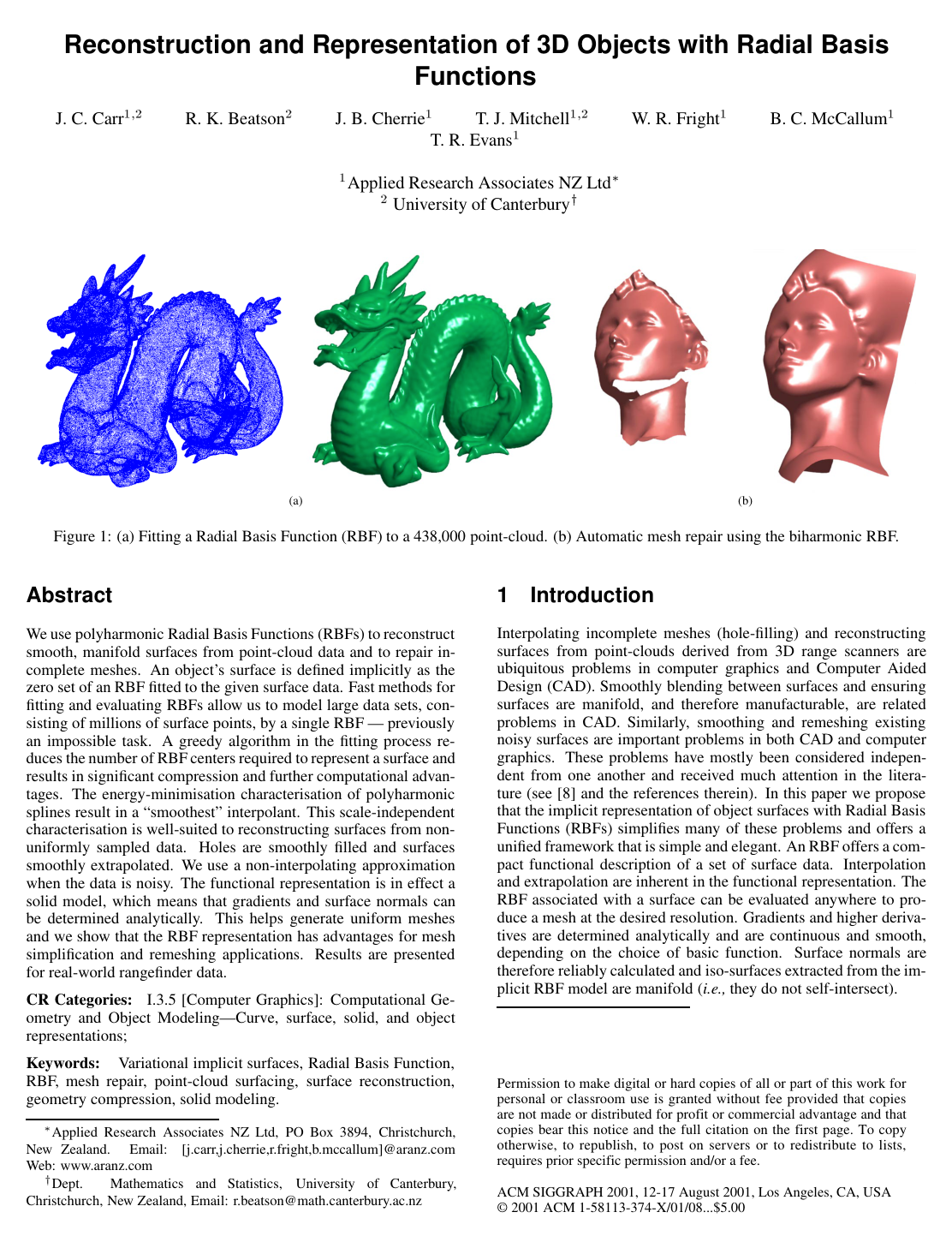
We use polyharmonic Radial Basis Functions (RBFs) to reconstruct smooth, manifold surfaces from point-cloud data and to repair incomplete meshes. An object's surface is defined implicitly as the zero set of an RBF fitted to the given surface data. Fast methods for fitting and evaluating RBFs allow us to model large data sets, consisting of millions of surface points, by a single RBF—previously an impossible task. A greedy algorithm in the fitting process reduces the number of RBF centers required to represent a surface and results in significant compression and further computational advantages. The energy-minimisation characterisation of polyharmonic splines result in a “smoothest” interpolant. This scale-independent characterisation is well-suited to reconstructing surfaces from non-uniformly sampled data. Holes are smoothly filled and surfaces smoothly extrapolated. We use a non-interpolating approximation when the data is noisy. The functional representation is in effect a solid model, which means that gradients and surface normals can be determined analytically. This helps generate uniform meshes and we show that the RBF representation has advantages for mesh simplification and remeshing applications. Results are presented for real-world rangefinder data.

Topics

cloud data point cloud reconstruction splines sampled-data rbf network multilayer perceptrons laser range finders

Keywords

Data RBF Surface Points Radial Basis Functions Representation Tting Objects Function

1 Introduction
1.1 Implicit surfaces
2 Fitting an implicit function to a surface
3 Radial Basis Function interpolation
4 Fast methods
5 RBF center reduction
6 RBF approximation of noisy data
7 Surface evaluation
8 Results
9 Summary and future work
10 Acknowledgements
References

Knowls

Knowl 1 — Implicit Surface Construction with Signed-Distance Off-Surface Constraints
model/method
To reconstruct an unknown surface $M \subset \mathbb{R}^3$ from $n$ distinct surface points $\{x_i\}_{i=1}^n$ , the surface is modeled as the zero-level set of an implicit function $f: \mathbb{R}^3 \to \mathbb{R}$ such that $f(x_i) = 0$ for $i=1,\dots,n$ .

To eliminate the trivial solution $f(x) \equiv 0$ , the dataset is augmented with $N - n$ off-surface points $\{x_i\}_{i=n+1}^N$ with non-zero values $f(x_i) = d_i \neq 0$ , creating a scattered data interpolation problem over $N$ total nodes. The target values $d_i$ are signed Euclidean distances to the closest on-surface point, assigned positive signs outside the object and negative signs inside.

Off-surface points are generated by projecting outward and inward along estimated surface unit normals $n_i$ at distance $|d_i|$ . To prevent artificial distortions where opposing surfaces are close (such as adjacent fingers), projection distances are validated dynamically to guarantee that the closest surface point to an off-surface point is the specific surface point that generated it. When normal directions or orientations cannot be reliably determined in sparse or unorganized point clouds, normal constraints are omitted at those locations, allowing the zero-surface constraints to determine the local field shape.
Knowl 2 — Biharmonic Radial Basis Function Interpolation System
theoretical result
Given $N$ distinct nodes $X = \{x_i\}_{i=1}^N \subset \mathbb{R}^3$ and target values $\{f_i\}_{i=1}^N \subset \mathbb{R}$ , the smoothest interpolant $s(x)$ minimizing the rotation-invariant Beppo-Levi second-derivative energy semi-norm:

$\|s\|^2 = \int_{\mathbb{R}^3} \left[ \left(\frac{\partial^2 s(x)}{\partial x^2}\right)^2 + \left(\frac{\partial^2 s(x)}{\partial y^2}\right)^2 + \left(\frac{\partial^2 s(x)}{\partial z^2}\right)^2 + 2\left(\frac{\partial^2 s(x)}{\partial x \partial y}\right)^2 + 2\left(\frac{\partial^2 s(x)}{\partial x \partial z}\right)^2 + 2\left(\frac{\partial^2 s(x)}{\partial y \partial z}\right)^2 \right] dx$

is given by the 3D biharmonic Radial Basis Function (RBF):

$s(x) = p(x) + \sum_{i=1}^N \lambda_i \|x - x_i\|$

where $\|\cdot\|$ is the Euclidean norm in $\mathbb{R}^3$ , $\lambda_i \in \mathbb{R}$ , and $p(x) = c_1 + c_2 x + c_3 y + c_4 z$ is a degree-1 polynomial with coefficients $c = (c_1, c_2, c_3, c_4)^T \in \mathbb{R}^4$ .

To satisfy membership in the Beppo-Levi distribution space $BL^{(2)}(\mathbb{R}^3)$ , the coefficients must satisfy the linear side conditions $\sum_{i=1}^N \lambda_i q(x_i) = 0$ for all polynomials $q$ of degree at most 1:

$\sum_{i=1}^N \lambda_i = 0, \quad \sum_{i=1}^N \lambda_i x_{i,1} = 0, \quad \sum_{i=1}^N \lambda_i x_{i,2} = 0, \quad \sum_{i=1}^N \lambda_i x_{i,3} = 0$

Combining the interpolation equations $s(x_i) = f_i$ for $i=1,\dots,N$ with these side conditions produces the symmetric $(N+4) \times (N+4)$ linear system:

$\begin{pmatrix} A & P \\ P^T & 0 \end{pmatrix} \begin{pmatrix} \lambda \\ c \end{pmatrix} = \begin{pmatrix} f \\ 0 \end{pmatrix}$

where $A_{i,j} = \|x_i - x_j\|$ for $i,j=1,\dots,N$ , $P \in \mathbb{R}^{N \times 4}$ has $i$ -th row $(1, x_{i,1}, x_{i,2}, x_{i,3})$ , $\lambda = (\lambda_1, \dots, \lambda_N)^T$ , and $f = (f_1, \dots, f_N)^T$ .
Knowl 3 — Regularized RBF Approximation for Noisy Surface Point Clouds
equation
For noisy surface data (such as 3D LIDAR scans), exact interpolation is replaced by a variational spline smoothing formulation that balances energy minimization against data fidelity:

$\min_{s \in BL^{(2)}(\mathbb{R}^3)} \rho \|s\|^2 + \frac{1}{N} \sum_{i=1}^N \left(s(x_i) - f_i\right)^2$

where $\|s\|^2$ is the Beppo-Levi rotation-invariant second-derivative energy semi-norm, $N$ is the number of data nodes, $f_i$ are target signed distances at coordinates $x_i \in \mathbb{R}^3$ , and $\rho \ge 0$ is a scalar stiffness parameter balancing smoothness against fidelity.

The unique minimizer retains the biharmonic form $s(x) = p(x) + \sum_{i=1}^N \lambda_i \|x - x_i\|$ , where the coefficients $\lambda \in \mathbb{R}^N$ and $c \in \mathbb{R}^4$ are determined by the linear system:

$\begin{pmatrix} A - 8 N \pi \rho I & P \\ P^T & 0 \end{pmatrix} \begin{pmatrix} \lambda \\ c \end{pmatrix} = \begin{pmatrix} f \\ 0 \end{pmatrix}$

where $A_{i,j} = \|x_i - x_j\|$ , $I$ is the $N \times N$ identity matrix, $P \in \mathbb{R}^{N \times 4}$ contains the linear polynomial basis evaluated at each node, $f = (f_1, \dots, f_N)^T$ , and $P^T \lambda = 0$ . Individual smoothing parameters $\rho_i$ may also be specified per node or point cluster.
Knowl 4 — Greedy Center Reduction for Sparse RBF Reconstruction
algorithm
An iterative algorithm reduces the number of RBF centers needed to represent a surface while guaranteeing that the approximation error at all $N$ data points remains within a prescribed error tolerance.
Input: Nodes $X = \{x_i\}_{i=1}^N$ , target values $\{f_i\}_{i=1}^N$ , fitting tolerance $\epsilon$ (or per-node tolerances $\{\epsilon_i\}_{i=1}^N$ )
Output: Reduced center set $C \subset X$ , polynomial coefficients $c$ , RBF weights $\lambda$
Choose an initial small subset of centers $C \subset X$
Fit an initial RBF $s(x)$ using only centers $C$ by solving the RBF linear system
loop
    Compute residuals $e_i = |f_i - s(x_i)|$ for all $i = 1, \dots, N$
    if $\max_{1 \le i \le N} e_i < \epsilon$ (or $e_i < \epsilon_i$ for all $i$ ) then
        return centers $C$ , weights $\lambda$ , and polynomial coefficients $c$
    end if
    Identify nodes $x_k \in X \setminus C$ where $e_k$ is large
    Update center set: $C \leftarrow C \cup \{x_k\}$
    Re-fit RBF $s(x)$ on the updated center set $C$
end loop
The algorithm reduces the required center count by up to an order of magnitude on dense laser scans. Because early iterations solve much smaller systems, center reduction frequently yields faster overall fitting times than fitting to all nodes directly.
Knowl 5 — Asymptotic Complexity and Scalability of Fast Multipole RBF Methods
theoretical result
Direct matrix methods for fitting and evaluating polyharmonic Radial Basis Functions (RBFs) require $O(N^2)$ memory storage for the interpolation matrix, $N^3/6 + O(N^2)$ floating point operations (flops) for Cholesky or symmetric factorization, and $O(N)$ operations per evaluation point.

By employing the Fast Multipole Method (FMM) adapted for 3D polyharmonic splines alongside preconditioned iterative solvers (such as preconditioned GMRES), computational and storage bounds are reduced to:
- Fitting memory storage: $O(N)$ , compared to $N(N+1)/2$ for direct solvers.
- Fitting computation: $O(N \log N)$ flops, compared to $N^3/6 + O(N^2)$ flops for direct solvers.
- Point evaluation: $O(1)$ flops per evaluation after an $O(N \log N)$ setup phase, compared to $O(N)$ flops per point for direct evaluation.
Simultaneous computation of the analytic gradient $\nabla s(x)$ with $s(x)$ requires approximately twice the computation of evaluating $s(x)$ alone. The framework utilizes two distinct user parameters: a fitting accuracy (maximum allowed node residual) and an evaluation accuracy (FMM expansion truncation precision), where the evaluation accuracy is configured to be strictly finer than the fitting accuracy.
Knowl 6 — Gradient-Guided Surface-Following Iso-Surface Extraction
model/method
To extract explicit polygonal meshes from the implicit surface defined by $s(x) = 0$ without evaluating a full 3D volumetric grid (which scales cubically as $O(M^3)$ for grid resolution $M$ ), a surface-following regularized marching tetrahedra method is used:
1. Seed point initialization: RBF centers situated on or near the zero-surface serve as seed points for distinct surface components. For off-surface centers, root-finding along the analytic gradient $\nabla s(x)$ rapidly identifies the nearest zero-crossing because the signed-distance gradient magnitude satisfies $\|\nabla s(x)\| \approx 1$ near the boundary.
2. Wavefront polygonization: Triangular or quadrilateral facets propagate outward from seed points in advancing wavefronts until wavefronts merge or meet the bounding volume.
3. Computational efficiency: By restricting RBF evaluations to the vicinity of the active wavefront, computational scaling is reduced from volumetric $O(M^3)$ to surface-area $O(M^2)$ . Memory overhead is bounded because only active wavefront vertices need to be retained.
4. Mesh regularization: Regularized marching tetrahedra optimization prevents skinny, ill-conditioned triangles, producing high-aspect-ratio meshes, while analytical evaluations of $\nabla s(x)$ eliminate topological surfacing ambiguities.

Knowl 7 — Performance of Fast Biharmonic RBF Fitting and Surfacing on Complex Scan Datasets

data/table

Empirical runtime, memory, and accuracy measurements for biharmonic RBF fitting with greedy center reduction and surface-following iso-surface extraction, tested on a 550 MHz Pentium III processor with 512 MB RAM:

Model	Surface Points	Interpolation Nodes	RBF Centers	Peak RAM (MB)	Fitting Time	Surfacing Time	Relative Accuracy
Face	14,806	29,074	3,564	29	68 s	27 s	$7 \times 10^{-4}$
Hand	13,348	26,696	4,299	29	97 s	32 s	$1 \times 10^{-3}$
Dragon	437,645	872,487	72,461	306	2:51:09	0:04:40	$8 \times 10^{-4}$
Buddha	543,652	1,086,194	80,518	291	4:03:26	0:04:07	$5 \times 10^{-4}$
Cherub statue	331,135	662,269	83,293	187	3:09:06	0:06:41	$4 \times 10^{-4}$
Skeleton hand	327,323	654,645	85,468	188	3:08:44	0:04:04	$3 \times 10^{-4}$
LIDAR statue	345,910	518,864	518,864	390	3:08:21	0:25:39	$6 \times 10^{-3}$

These experiments demonstrate that datasets exceeding 500,000 surface points (generating over 1,000,000 interpolation nodes due to paired positive and negative off-surface constraints) can be reconstructed within 300 to 400 MB of peak core memory, whereas a direct dense linear solver for the Buddha dataset would require 4,700 GB just for matrix storage. Greedy center reduction reduces the required centers by $7\times$ to $13\times$ relative to node count while maintaining relative errors between $10^{-3}$ and $10^{-4}$ .

Knowl 8 — Geometric Compression and Storage Comparison for RBF Functional Models

data/table

Storage comparison between raw input polygon meshes, the continuous RBF functional representation, and newly remeshed models evaluated from the fitted RBFs. Uncompressed meshes allocate 12 bytes (3 single-precision floats) per vertex and 12 bytes (3 integers) per triangular face; uncompressed RBF models allocate 12 bytes per center coordinate and 8 bytes (1 double-precision float) per weight $\lambda_i$ :

Model	Original Mesh			New Mesh (from RBF)			RBF Representation
	Vertices	Facets	Storage	Vertices	Facets	Storage	Centers	Storage
Dragon	437,645	847,414	15.4 MB	126,998	254,016	4.5 MB	72,461	1.4 MB
Buddha	543,652	1,086,798	19.6 MB	96,766	193,604	3.5 MB	80,518	1.6 MB
Skeleton hand	327,323	654,666	11.8 MB	81,829	163,698	2.9 MB	85,468	1.7 MB

The continuous RBF representation compresses the surface description by approximately an order of magnitude relative to the raw input mesh (e.g., 15.4 MB down to 1.4 MB for Dragon, 19.6 MB down to 1.6 MB for Buddha). Re-evaluating the implicit function produces uniform, hole-free meshes that capture all surface detail using less than one-third of the original facet count.

Knowl 9 — Automatic Mesh Repair and Hole-Filling via Biharmonic Spline Extrapolation
empirical result
Because biharmonic RBFs minimize a global second-derivative energy functional across $\mathbb{R}^3$ , implicit surface fitting inherently extrapolates missing surface regions across scanning occlusions, shadows, and partial meshes without requiring explicit hole detection, topological surgery, or boundary curve stitching.

When applied to partial laser scans containing large irregular voids (such as occluded regions under a chin, or hidden contact zones between embracing figures in multi-part statues), the fitted biharmonic RBF automatically generates closed, watertight, 2-manifold surfaces that smoothly bridge missing data according to surrounding curvature trends. In statue scans with severe occlusions, missing anatomical features (such as missing chest sections inferred from adjacent shoulder data) are reconstructed smoothly while separate, closely spaced limbs remain topologically distinct without spurious bridging.
Knowl 10 — Trade-offs and Limitations of Global Polyharmonic RBF Representations
limitation
While global polyharmonic RBFs offer smooth interpolation and parameterization-free reconstruction, they present distinct operational trade-offs:
1. Global coupling: Because the biharmonic basis function $\phi(r) = r$ has infinite support, modifying or adding a local point constraint alters the implicit field value $s(x)$ everywhere. Local geometric manipulation and direct ray tracing require root-searching across the global sum rather than evaluating localized patches.
2. Center scaling on high-genus internal structures: Representing intricate internal geometries with high topological genus (such as a hollow turbine blade with complex cooling channels) requires hundreds of thousands of centers (e.g., 594,000 centers for a single blade), demanding high computational effort and continuous reliance on FMM acceleration.
3. Normal validation sensitivity: In thin geometries or closely situated opposing surfaces, inaccurate surface normal lengths cause off-surface points from opposite sides to intersect, corrupting the zero-level set unless rigorous dynamic distance validation is enforced.

Coverage note — None was omitted; all primary theoretical formulations, algorithms, computational performance data, compression analyses, mesh repair results, and limitations are fully covered.

References

1.C. Bajaj, J. Chen, and G. Xu. Modeling with cubic a-patches. ACM Transactions on Computer Graphics, 14(2):103–133, 1995.
2.R. K. Beatson, J. B. Cherrie, and C. T. Mouat. Fast fitting of radial basis functions: Methods based on preconditioned GMRES iteration. Advances in Computational Mathematics, 11:253–270, 1999.
3.R. K. Beatson, J. B. Cherrie, and D. L. Ragozin. Fast evaluation of radial basis functions: Methods for four-dimensional polyharmonic splines. SIAM J. Math. Anal., 32(6):1272–1310, 2001.
4.R. K. Beatson and L. Greengard. A short course on fast multipole methods. In M. Ainsworth, J. Levesley, W.A. Light, and M. Marletta, editors, Wavelets, Multilevel Methods and Elliptic PDEs, pages 1–37. Oxford University Press, 1997.
5.R. K. Beatson and W. A. Light. Fast evaluation of radial basis functions: Methods for two-dimensional polyharmonic splines. IMA Journal of Numerical Analysis, 17:343–372, 1997.
6.R. K. Beatson, W. A. Light, and S. Billings. Fast solution of the radial basis function interpolation equations: Domain decomposition methods. SIAM J. Sci. Comput., 22(5):1717–1740, 2000.
7.R. K. Beatson, A. M. Tan, and M. J. D. Powell. Fast evaluation of radial basis functions: Methods for 3-dimensional polyharmonic splines. In preparation.
8.F. Bernardini, C. L. Bajaj, J. Chen, and D. R. Schikore. Automatic reconstruction of 3D CAD models from digital scans. Int. J. on Comp. Geom. and Appl., 9(4–5):327, Aug & Oct 1999.
9.J. Bloomenthal, editor. Introduction to Implicit Surfaces. Morgan Kaufmann, San Francisco, California, 1997.
10.J. C. Carr, W. R. Fright, and R. K. Beatson. Surface interpolation with radial basis functions for medical imaging. IEEE Trans. Medical Imaging, 16(1):96–107, February 1997.
11.E. W. Cheney and W. A. Light. A Course in Approximation Theory. Brooks Cole, Pacific Grove, 1999.
12.J. Duchon. Splines minimizing rotation-invariant semi-norms in Sobolev spaces. In W. Schempp and K. Zeller, editors, Constructive Theory of Functions of Several Variables, number 571 in Lecture Notes in Mathematics, pages 85–100, Berlin, 1977. Springer-Verlag.
13.N. Dyn, D. Levin, and S. Rippa. Numerical procedures for surface fitting of scattered data by radial functions. SIAM J. Sci. Stat. Comput., 7(2):639–659, 1986.
14.J. Flusser. An adaptive method for image registration. Pattern Recognition, 25(1):45–54, 1992.
15.L. Greengard and V. Rokhlin. A fast algorithm for particle simulations. J. Comput. Phys, 73:325–348, 1987.
16.H. Hoppe, T. DeRose, T. Duchamp, J. McDonald, and W. Stuetzle. Surface reconstuction from unorganized points. Computer Graphics (SIGGRAPH’92 proceedings), 26(2):71–78, July 1992.
17.W. E. Lorensen and H. E. Cline. Marching cubes: A high resolution 3D surface construction algorithm. Computer Graphics, 21(4):163–169, July 1987.
18.C. A. Micchelli. Interpolation of scattered data: Distance matrices and conditionally positive definite functions. Constr. Approx., 2:11–22, 1986.
19.V. V. Savchenko, A. A. Pasko, O. G. Okunev, and T. L. Kunii. Function representation of solids reconstructed from scattered surface points and contours. Computer Graphics Forum, 14(4):181–188, 1995.
20.R. Sibson and G. Stone. Computation of thin-plate splines. SIAM J. Sci. Stat. Comput., 12(6):1304–1313, 1991.
21.G. M. Treece, R. W. Prager, and A. H. Gee. Regularised marching tetrahedra: improved iso-surface extraction. Computers and Graphics, 23(4):583–598, 1999.
22.G. Turk and J. F. O’Brien. Shape transformation using variational implicit surfaces. In SIGGRAPH’99, pages 335–342, Aug 1999.
23.G. Turk and J. F. O’Brien. Variational implicit surfaces. Technical Report GIT-GVU-99-15, Georgia Institute of Technology, May 1999.
24.G. Wahba. Spline Models for Observational Data. Number 59 in CBMS-NSF Regional Conference Series in Applied Math. SIAM, 1990.
25.G. Yngve and G. Turk. Creating smooth implicit surfaces from polygonal meshes. Technical Report GIT-GVU-99-42, Georgia Institute of Technology, 1999.

Citation

MLA

Carr, J. C., et al. “Reconstruction and Representation of 3D Objects with Radial Basis Functions”. Proceedings of the 28th Annual Conference on Computer Graphics and Interactive Techniques, 2001, pp. 67–76, https://doi.org/10.1145/383259.383266.

APA

Carr, J. C., Beatson, R. K., Cherrie, J. B., Mitchell, T. J., Fright, W. R., McCallum, B. C., & Evans, T. R. (2001). Reconstruction and representation of 3D objects with radial basis functions. Proceedings of the 28th Annual Conference on Computer Graphics and Interactive Techniques, 67–76. https://doi.org/10.1145/383259.383266

Chicago

Carr, J. C., R. K. Beatson, J. B. Cherrie, et al. 2001. “Reconstruction and Representation of 3D Objects with Radial Basis Functions”. Proceedings of the 28th Annual Conference on Computer Graphics and Interactive Techniques, 67–76. https://doi.org/10.1145/383259.383266.

Harvard

Carr, J.C. et al. (2001) “Reconstruction and representation of 3D objects with radial basis functions”, Proceedings of the 28th annual conference on Computer graphics and interactive techniques. ACM, pp. 67–76. Available at: https://doi.org/10.1145/383259.383266.

Vancouver

1. Carr JC, Beatson RK, Cherrie JB, Mitchell TJ, Fright WR, McCallum BC, Evans TR (2001) Reconstruction and representation of 3D objects with radial basis functions. In: Proceedings of the 28th annual conference on Computer graphics and interactive techniques. ACM, pp 67–76

BibTeX

@inproceedings{Carr_2001, series={SIGGRAPH01}, title={Reconstruction and representation of 3D objects with radial basis functions}, url={http://dx.doi.org/10.1145/383259.383266}, DOI={10.1145/383259.383266}, booktitle={Proceedings of the 28th annual conference on Computer graphics and interactive techniques}, publisher={ACM}, author={Carr, J. C. and Beatson, R. K. and Cherrie, J. B. and Mitchell, T. J. and Fright, W. R. and McCallum, B. C. and Evans, T. R.}, year={2001}, month=Aug, pages={67–76}, collection={SIGGRAPH01} }

Metadata:Crossref

Access the Paper

This paper is available from its original source. Click below to access the PDF.

Open PDF

Reconstruction and representation of 3D objects with radial basis functions

Abstract

Topics

Keywords

Table of Contents

Knowls

Knowl 1 — Implicit Surface Construction with Signed-Distance Off-Surface Constraints

Knowl 2 — Biharmonic Radial Basis Function Interpolation System

Knowl 3 — Regularized RBF Approximation for Noisy Surface Point Clouds

Knowl 4 — Greedy Center Reduction for Sparse RBF Reconstruction

Knowl 5 — Asymptotic Complexity and Scalability of Fast Multipole RBF Methods

Knowl 6 — Gradient-Guided Surface-Following Iso-Surface Extraction