Single image dehazing

Raanan Fattal

article2008TOG2,422 citations

Develops a single-image dehazing method that separates transmission from surface shading to restore contrast and support depth-aware applications.

Listen

Light scattering caused by atmospheric particles like fog, haze, and dust degrades photographs by muting surface colors, reducing contrast, and introducing a veil of scattered light known as airlight. This degradation severely limits image quality and visibility across satellite imaging, aerial cartography, underwater operations, and everyday photography. Restoring a clear, haze-free scene from a single standard photograph has historically been considered an underdetermined problem because it is mathematically impossible to distinguish whether a pixel appears pale due to heavy haze or inherently pale surface coloring without additional inputs.

The article aims to resolve this fundamental ambiguity and demonstrate an automated, passive method to restore clear visibility and estimate medium transmission directly from a single standard input image without requiring specialized optical sensors, user interaction, multiple views, or prior depth data.

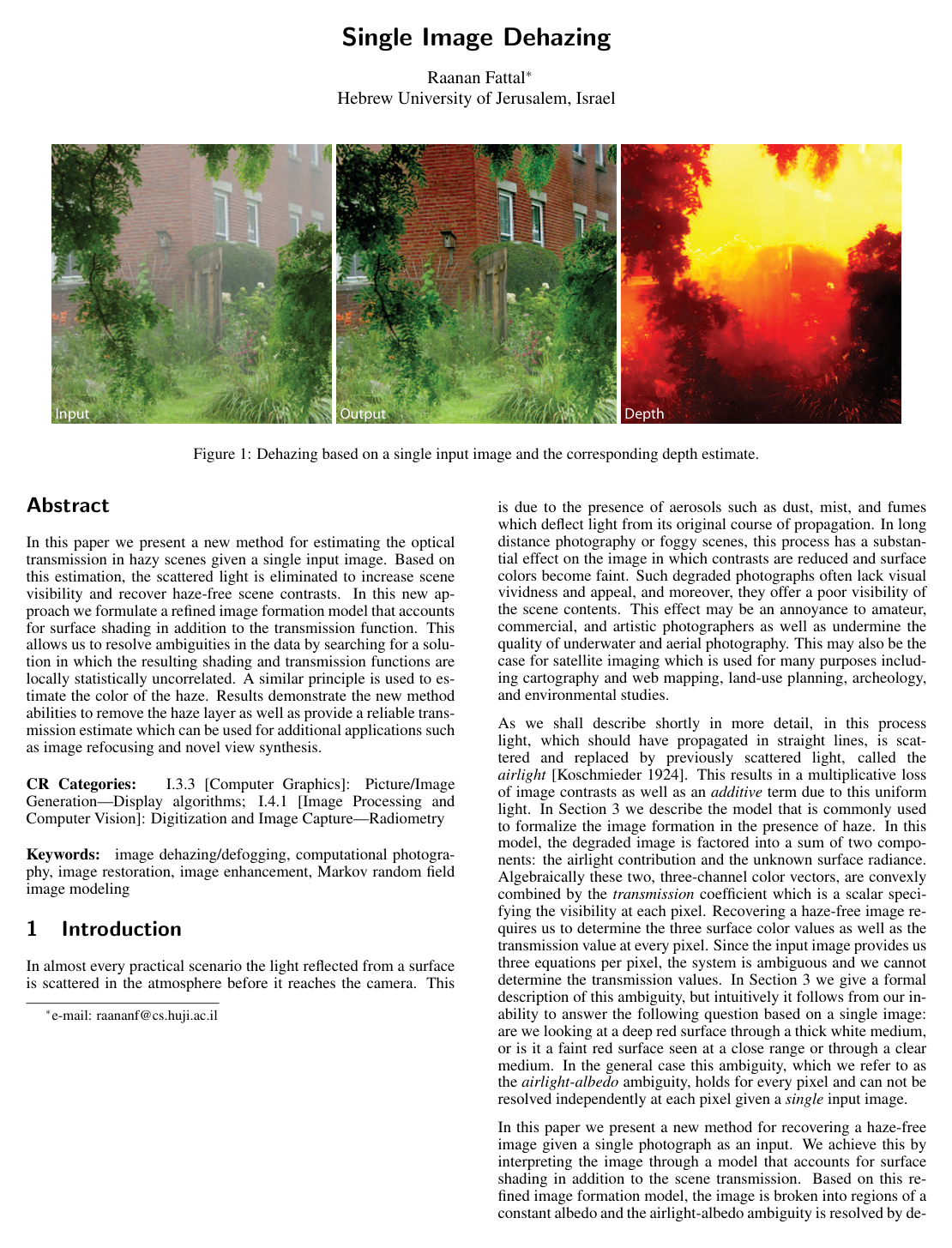
The approach introduces a refined physical model that factors surface appearance into lighting, shading, and underlying material properties. By observing that variations in natural surface shading and changes in atmospheric medium transmission are statistically uncorrelated across local image regions, the method isolates and removes the haze layer. To handle complex scenes containing multiple surface colors and textures, the technique incorporates robust statistical estimators within local neighborhoods and applies a Markov random field model to infer transmission across noisy or ambiguous areas.

Key findings confirm that this statistical approach successfully decouples the haze component from surface radiance. In validation tests against ground-truth benchmarks, the method achieved high accuracy, maintaining a mean absolute error below seven percent for both the estimated transmission and the restored haze-free images. Furthermore, the algorithm matched the visibility quality of multi-image polarization systems while avoiding the severe halo artifacts and residual airlight commonly left behind by conventional contrast enhancement, dark-object subtraction, and tone-mapping techniques. The process is computationally practical, requiring approximately 35 seconds to restore a 512-by-512 pixel image on standard dual-core consumer computing hardware.

These results establish that high-quality dehazing and scene-depth extraction can be achieved passively using ordinary consumer hardware, eliminating the need for expensive multi-sensor arrays or manual user inputs. This offers substantial performance improvements and cost reductions for automated computer vision systems operating under adverse weather conditions. Additionally, the recovered depth and transmission data enable secondary imaging applications, such as synthetic depth-of-field refocusing, novel view synthesis, and controlled atmospheric fog simulation.

Decision-makers and practitioners working with remote sensing, surveillance, or consumer photography pipelines can adopt this framework directly without optical hardware modifications. To transition toward deployment, future work should explore integrating deblurring mechanisms directly with transmission estimation to mitigate atmospheric optical blur. However, caution is advised in heavily degraded scenes with low signal-to-noise ratios or flat, textureless surfaces where shading variation is insufficient, as these conditions violate the underlying statistical assumptions and lead to inaccurate transmission estimates.

The Hebrew University of Jerusalem color images optical transmissions view synthesis single image dehazing haze removal multi-scale bilateral filter

Fattal (2008).pdf

Paper: Digital Image Enhancement and Noise Filtering by Use of Local Statistics, Jong-Sen Lee (1980). Reading this foundational work on local statistics and minimum mean-square error filtering provides essential background for understanding spatial window operations in image restoration.
Paper: Guided Image Filtering, Kaiming He et al. (2010). Understanding the guided filter and its linear modeling of edge-preserving smoothing prepares the reader for spatial transmission estimation and refinement techniques.

Paper: DehazeNet: An End-to-End System for Single Image Haze Removal, Bolun Cai et al. (2016). This paper directly extends single-image dehazing by replacing hand-crafted transmission priors with an end-to-end convolutional neural network.

Abstract

In this paper we present a new method for estimating the optical transmission in hazy scenes given a single input image. Based on this estimation, the scattered light is eliminated to increase scene visibility and recover haze-free scene contrasts. In this new approach we formulate a refined image formation model that accounts for surface shading in addition to the transmission function. This allows us to resolve ambiguities in the data by searching for a solution in which the resulting shading and transmission functions are locally statistically uncorrelated. A similar principle is used to estimate the color of the haze. Results demonstrate the new method abilities to remove the haze layer as well as provide a reliable transmission estimate which can be used for additional applications such as image refocusing and novel view synthesis.

Topics

color images optical transmissions view synthesis image formations single images estimation method viewpoint

Keywords

single image dehazing haze removal multi-scale bilateral filter airlight-albedo ambiguity image restoration surface reflectance dark-object subtraction airlight color vector multiple scattering contrast enhancement

1 Introduction
2 Previous Work
3 Image Degradation Model
4 Constant Albedo Images
5 Noise Estimation
6 Multi-Albedo Images
7 Estimating the Airlight Color
8 Results
9 Conclusions
Acknowledgements
References
Appendix: Derivation of the Noise Estimates

Knowls

Knowl 1 — Airlight-Albedo Ambiguity Resolution via Shading-Transmission Uncorrelation
model/method
In single image dehazing, estimating the transmission $t(x) in [0, 1]$ and haze-free radiance $J(x) in \mathbb{R}^3$ from an observed RGB pixel $I(x) = t(x) J(x) + (1 - t(x)) A$ (where $A in \mathbb{R}^3$ is the airlight vector) is fundamentally underconstrained. Over a localized image region $\Omega$ sharing a constant surface albedo $R \in \mathbb{R}^3$ , the surface radiance is modeled as $J(x) = l(x) R$ , where $l(x) \in \mathbb{R}$ is the scalar shading factor.

Because scene transmission $t$ depends on geometry and medium density while shading $l$ depends on surface orientation and illumination, $t$ and $1/l'$ are assumed to be statistically uncorrelated over $\Omega$ , where $l'(x) = \|R'\| l(x)$ and $R'$ is the component of $R$ orthogonal to $A$ . Under this assumption, the sample covariance satisfies $C_\Omega(t, 1/l') = 0$ .

Defining the auxiliary variable: $h(x) = \frac{\|A\| - I_A(x)}{I_{R'}(x)}$ where $I_A(x) = \langle I(x), A \rangle / \|A\|$ is the projection of the pixel along $A$ and $I_{R'}(x) = \sqrt{\|I(x)\|^2 - I_A(x)^2}$ is the orthogonal norm, the unknown scalar parameter $\eta = \langle R, A \rangle / (\|R'\| \|A\|)$ is uniquely resolved as: $\eta = \frac{C_\Omega(I_A, h)}{C_\Omega(I_{R'}, h)}$ where for any fields $f$ and $g$ , $C_\Omega(f, g) = |\Omega|^{-1} \sum_{x \in \Omega} (f(x) - E_\Omega(f))(g(x) - E_\Omega(g))$ and $E_\Omega(f) = |\Omega|^{-1} \sum_{x \in \Omega} f(x)$ . Once $\eta$ is known, the transmission is given by: $t(x) = 1 - \frac{I_A(x) - \eta I_{R'}(x)}{\|A\|}$
Knowl 2 — Constant-Albedo Image Formation and Orthogonal Decomposition
model/method
Under the standard physical model of atmospheric scattering, the observed RGB color $I(x)$ at pixel $x$ is formed by: $I(x) = t(x) J(x) + (1 - t(x)) A$ where $A \in \mathbb{R}^3$ is the uniform airlight color vector, $t(x) \in [0, 1]$ is the medium transmission, and $J(x) \in \mathbb{R}^3$ is the surface radiance. For a region with constant surface albedo vector $R \in \mathbb{R}^3$ , the surface radiance is factored into $J(x) = l(x) R$ with scalar shading $l(x)$ .

The albedo vector $R$ is decomposed into a component parallel to $A$ and an orthogonal residual $R' \in A^\perp$ ( $R' \perp A$ ): $R = R' + \eta \|R'\| \frac{A}{\|A\|}$ where $\eta = \frac{\langle R, A \rangle}{\|R'\| \|A\|}$ measures the mutual component between the surface albedo and the airlight. Defining $l'(x) = \|R'\| l(x)$ , the image formation equation becomes: $I(x) = t(x) l'(x) \left( \frac{R'}{\|R'\|} + \eta \frac{A}{\|A\|} \right) + (1 - t(x)) A$

Projecting $I(x)$ parallel and orthogonal to $A$ yields two scalar observations per pixel: $I_A(x) = \frac{\langle I(x), A \rangle}{\|A\|} = t(x) l'(x) \eta + (1 - t(x)) \|A\|$ $I_{R'}(x) = \sqrt{\|I(x)\|^2 - I_A(x)^2} = t(x) l'(x)$

Solving for transmission yields $t(x) = 1 - \frac{I_A(x) - \eta I_{R'}(x)}{\|A\|}$ and solving for inverse shading yields $(l'(x))^{-1} = \frac{1 - I_A(x)/\|A\|}{I_{R'}(x)} + \frac{\eta}{\|A\|}$ .
Knowl 3 — Multi-Albedo Weighting via Shading- and Airlight-Invariant Chromaticity
model/method
To handle images with spatially varying albedo, local statistics are computed using robust $w$ -estimators that weight neighboring pixels by chromaticity similarity rather than shading.

A shading- and airlight-invariant chromaticity angle $\theta(x)$ is computed by projecting a haze-subtracted vector $I'(x) = I(x) - A \frac{I_A(x)}{\|A\|}$ onto the $U$ and $V$ chroma channels of the YUV color space: $\theta(x) = \tan^{-1}\left( \frac{\langle I'(x), U \rangle}{\langle I'(x), V \rangle} \right)$

The angular distance between two chromaticity angles is defined on the circle by: $d(\theta_1, \theta_2) = \min(|\theta_1 - \theta_2|, 2\pi - |\theta_1 - \theta_2|)$

For each pixel $x$ , the robust local mean $E_x(f)$ and sample covariance $C_x(f, g)$ are evaluated over a spatial window $\Omega_x$ (typically $24 \times 24$ pixels) centered at $x$ , excluding unreliable pixels belonging to the set $\mathcal{B}$ : $E_x(f) = \frac{1}{W_x} \sum_{y \in \Omega_x} f(y) w(x, y)$ $C_x(f, g) = \frac{1}{W_x} \sum_{y \in \Omega_x} (f(y) - E_x(f))(g(y) - E_x(g)) w(x, y)$ where $w(x, y) = \exp\left( - \frac{d(\theta(x), \theta(y))^2}{\sigma_\theta^2} \right)$ , $W_x = \sum_{y \in \Omega_x} w(x, y)$ , and $\sigma_\theta = 1/8$ .

The per-pixel albedo-airlight mutual coefficient is $\eta(x) = \frac{C_x(I_A, h)}{C_x(I_{R'}, h)}$ , yielding the primary transmission estimate $\hat{t}(x) = 1 - \frac{I_A(x) - \eta(x) I_{R'}(x)}{\|A\|}$ for all $x \notin \mathcal{B}$ .
Knowl 4 — Gauss-Markov Random Field Transmission Regularization and Propagation
model/method
To account for estimation noise in the primary transmission estimates $\hat{t}(x)$ and propagate transmission to unreliable pixels $x \in \mathcal{B}$ , a Gauss-Markov Random Field (GMRF) model is defined over the entire image lattice: $P(t) \propto \prod_{x \notin \mathcal{B}} \exp\left( - \frac{(t(x) - \hat{t}(x))^2}{\sigma_t^2(x)} \right) \prod_{\forall x, y \in N_x} \exp\left( - \frac{(t(x) - t(y))^2}{(I_A(x) - I_A(y))^2 / \sigma_s^2} \right)$ where $N_x$ is the 4-nearest neighborhood of pixel $x$ , $\sigma_t^2(x)$ is the analytically derived variance of the noise in $\hat{t}(x)$ , and $\sigma_s = 1/5$ sets the smoothness scale. Spatial smoothness is weighted inversely by the gradient in the airlight projection $I_A(x)$ , preserving transmission edges that coincide with airlight steps.

The maximum a posteriori transmission map $t$ is computed by setting $\frac{\partial \log P(t)}{\partial t} = 0$ , which yields a linear system of equations. Once solved for $t(x)$ , the final haze-free image $J(x)$ is reconstructed via: $J(x) = \frac{I(x) - (1 - t(x))A}{t(x)}$
Knowl 5 — Noise Variance Propagation and Transmission Admissibility Criteria
theoretical result
Assuming input image noise is zero-mean additive white Gaussian noise $I(x) = \tilde{I}(x) + \xi(x)$ with $\xi(x) \sim \mathcal{N}(0, \sigma^2 I_{3 \times 3})$ , linearizing error propagation through first-order Taylor expansion yields a zero-mean Gaussian error $\xi_t(x)$ in the transmission estimate: $\xi_t(x) = \frac{\xi_A(x) - \tilde{\eta}(x) \xi_{R'}(x) - \tilde{I}_{R'}(x) \xi_\eta(x)}{\|A\|}$ with variance $\sigma_t^2(x) = \text{Var}_\xi(\xi_t(x))$ .

A pixel $x$ is flagged as unreliable and assigned to the discarded set $\mathcal{B}$ if any of the following conditions required for Taylor series truncation and statistical stability fail:
1. $\sigma \ge I_c(x) / 10$ for any color channel $c \in \{R, G, B\}$ .
2. $\sigma \ge I_{R'}(x) / 6$ , where $I_{R'}$ is the haze-free component.
3. $\text{Var}_\xi(\xi_{C_{R'}}) \ge \left( \frac{C_{\Omega_x}(I_{R'}, h)}{5} \right)^2$ , where $\xi_{C_{R'}}$ is the noise in the covariance denominator $C_{\Omega_x}(I_{R'}, h)$ .
In typical implementations, $\sigma$ is set in the range $[1/200, 1/100]$ for pixel values normalized in $[0, 1]$ .
Knowl 6 — Airlight Color Vector Estimation via Subspace Intersection and Covariance Minimization
algorithm
The airlight color vector $A \in \mathbb{R}^3$ can be determined from two or more regions of uniform albedo using subspace intersection followed by a 1D covariance search.
Input: Observed image $I$ , set of $K \ge 2$ uniform-albedo regions $\{\Omega_i\}_{i=1}^K$
Output: Airlight color vector $A \in \mathbb{R}^3$
for each region $i = 1$ to $K$ do
Perform PCA on the RGB radiances $\{I(x) : x \in \Omega_i\}$
Extract the two principal eigenvectors $v_1^i, v_2^i \in \mathbb{R}^3$ corresponding to the largest eigenvalues
end for
Construct the $3 \times 3$ matrix $M = \sum_{i=1}^K \left( v_1^i (v_1^i)^T + v_2^i (v_2^i)^T \right)$
Find unit vector $\hat{A} = \arg\max_{\|u\|=1} u^T M u$ as the eigenvector of $M$ corresponding to its maximum eigenvalue
Perform a 1D line search over scalar magnitude $\|A\| > 0$ to minimize $(C(J, t))^2$ over local windows, where $A = \|A\| \hat{A}$
return $A$
If distinct uniform regions are unavailable, a full 3D optimization is used: $A$ is initialized to the most haze-opaque pixel and updated via steepest descent to minimize $(C(J, t))^2$ within $24 \times 24$ pixel windows.
Knowl 7 — Transmission-Based Depth Estimation, Refocusing, and Fog Modulation
model/method
The recovered transmission field $t(x) = \exp\left( -\int_0^{d(x)} \beta(s) ds \right)$ enables synthetic depth-based image manipulations:
1. Relative Depth Recovery: Under the assumption of a spatially uniform medium extinction coefficient $\beta(s) = \beta$ , the scene depth $d(x)$ is computed up to an unknown global scale factor $1/\beta$ : $d(x) = -\frac{\log t(x)}{\beta}$
2. Haze Density Adjustment: Simulating a medium with extinction coefficient scaled by a factor $\lambda$ corresponds to a power-law transformation of the transmission values: $t_\lambda(x) = (t(x))^\lambda$
3. Haze Recoloring and Perturbation: The fog layer $(1 - t(x))A$ can be recolored by replacing $A$ with an arbitrary color vector $A_{\text{new}}$ , or spatially modulated by multiplying the haze term with multi-scale random noise.
4. Synthetic Refocusing: The recovered relative depth map $d(x)$ can be used to define a virtual focal plane and apply spatially varying depth-of-field blur.
Knowl 8 — Dehazing Limitations Under Insufficient Shading Variation and Low SNR
limitation
The method relies fundamentally on the existence of significant multiplicative shading variations to decorrelate shading from transmission. The approach fails or degrades under the following conditions:
1. Vanishing Orthogonal Component ( $I_{R'} \approx 0$ ): When a surface albedo vector $R$ is nearly parallel to the airlight vector $A$ , the orthogonal residual norm $I_{R'}(x)$ approaches zero, leading to severe division-by-zero overshoots in the transmission calculation $t(x) = 1 - (I_A(x) - \eta I_{R'}(x))/\|A\|$ .
2. Zero Covariance Denominator ( $C(I_{R'}, h) \approx 0$ ): On flat, textureless surfaces with uniform lighting and albedo, shading variation is absent, causing the covariance denominator to vanish and rendering $\eta$ indeterminate.
3. Low Signal-to-Noise Ratio: In regions of dense fog or deep shadows where the haze-free radiance $J(x)$ falls below camera noise $\sigma$ , the signal cannot be recovered.
4. Under-Sampled Albedos: Isolated structures with distinct albedos containing too few pixels undermine the statistical sample size required for stable covariance estimation.

Coverage note — No substantial contributed material was omitted. Specific hardware runtime benchmarks (35 seconds for 512x512 on a 1.6GHz CPU) and basic qualitative visual comparisons against existing methods were condensed into the core algorithmic and limitation descriptions.

References

1.ANDREWS, D. F., BICKEL, P. J., HAMPEL, F. R., HUBER, P. J., ROGERS, W. H., AND W.TUKEY, J. 1972. Robust Estimates of Location: Survey and Advances. Princeton University Press; London, Oxford University Press.
2.CHAVEZ, P. S. 1988. An improved dark-object subtraction technique for atmonspheric scattering correction of multispectral data. Remote Sensing of Environment 24, 450–479.
3.COON, D. 2005. Psychology: A Modular Approach To Mind And Behavior. Wadsworth Pub Co, July.
4.DEBEVEC, P. E., AND MALIK, J. 1997. Recovering high dynamic range radiance maps from photographs. In ACM SIGGRAPH 1997, 369–378.
5.DU, Y., GUINDON, B., AND CIHLAR, J. 2002. Haze detection and removal in high resolution satellite image with wavelet analysis. IEEE Transactions on Geoscience and Remote Sensing 40, 1, 210–217.
6.FATTAL, R., AGRAWALA, M., AND RUSINKIEWICZ, S. 2007. Multiscale shape and detail enhancement from multi-light image collections. In ACM SIGGRAPH, 51.
7.FATTAL, R. 2007. Image upsampling via imposed edge statistics. ACM SIGGRAPH 26, 3, 95.
8.GREWE, L., AND BROOKS, R. R. 1998. Atmospheric attenuation reduction through multi-sensor fusion in sensor fusion: Architectures, algorithms, and applications. 102–109.
9.HIRSCHMLLER, H., AND SCHARSTEIN, D. 2007. Evaluation of cost functions for stereo matching.
10.HYVRINEN, A., AND OJA, E. 2000. Independent component analysis: Algorithms and applications. Neural Networks 13, 411–430.
11.KOSCHMIEDER, H. 1924. Theorie der horizontalen sichtweite. In Beitr. zur Phys. d. freien Atm., 171–181.
12.LARSON, G. W., RUSHMEIER, H., AND PIATKO, C. 1997. A visibility matching tone reproduction operator for high dynamic range scenes. IEEE Transactions on Visualization and Computer Graphics 3, 4, 291–306.
13.LEVIN, A., FERGUS, R., DURAND, F., AND FREEMAN, W. T. 2007. Image and depth from a conventional camera with a coded aperture. ACM Transaction on Graphics 26, 3, 70.
14.LIU, C., FREEMAN, W. T., SZELISKI, R., AND KANG, S. B. 2006. Noise estimation from a single image. In Proceedings of IEEE CVPR, 901–908.
15.LU, J., AND JR., D. M. H. 1994. Contrast enhancement via multiscale gradient transformation. In IEEE International Conference on Image Processing, 482–486.
16.NARASIMHAN, S. G., AND NAYAR, S. K. 2000. Chromatic framework for vision in bad weather. In Proceedings of IEEE CVPR, 598–605.
17.NARASIMHAN, S. G., AND NAYAR, S. K. 2003. Interactive (De)weathering of an Image using Physical Models. In ICCV Workshop on Color and Photometric Methods in Computer Vision (CPMCV).
18.NAYAR, S. K., AND NARASIMHAN, S. G. 1999. Vision in bad weather. In Proceedings of IEEE CVPR, 820.
19.OAKLEY, J. P., AND BU, H. 2007. Correction of simple contrast loss in color images. IEEE Transactions on Image Processing 16, 2, 511–522.
20.PÉREZ, P. 1998. Markov random fields and images. In CWI Quarterly, vol. 11, 413–437.
21.RAHMAN, Z., JOBSON, D., AND WOODELL, G. 1996. Multiscale retinex for color image enhancement.
22.ROSSUM, M. V., AND NIEUWENHUIZEN, T. 1999. Multiple scattering of classical waves: microscopy, mesoscopy and diffusion. vol. 71, 313–371.
23.SCHECHNER, Y. Y., AND AVERBUCH, Y. 2007. Regularized image recovery in scattering media. IEEE Transactions on Pattern Analysis and Machine Intelligence 29, 9, 1655–1660.
24.SCHECHNER, Y. Y., NARASIMHAN, S. G., AND NAYAR, S. K. 2001. Instant dehazing of images using polarization. 325–332.
25.SHWARTZ, S., NAMER, E., Y., Y., AND SCHECHNER. 2006. Blind haze separation. In Proceedings of IEEE CVPR, 1984–1991.
26.SINGH, M., AND ANDERSON, B. 2002. Toward a perceptual theory of transparency. No. 109, 492–519.
27.TAN, K., AND OAKLEY, J. P. 2000. Enhancement of color images in poor visibility conditions. Proceedings of International Conference on Image Processing 2, 788–791.
28.TAN, R. T. 2008. Visibility in bad weather from a single image. Proceedings of IEEE CVPR.
29.VEERARAGHAVAN, A., RASKAR, R., AGRAWAL, A., MOHAN, A., AND TUMBLIN, J. 2007. Dappled photography: mask enhanced cameras for heterodyned light fields and coded aperture refocusing. In ACM SIGGRAPH, 69.
30.WIKIPEDIA, 2007. Unsharp masking — wikipedia, the free ency-clopedia.
31.YUAN, L., SUN, J., QUAN, L., AND SHUM, H.-Y. 2007. Image deblurring with blurred/noisy image pairs. ACM Transactions on Graphics 26, 3, 1.
32.ZHANG, Y., GUINDON, B., AND CIHLAR, J. 2002. An image transform to characterize and compensate for spatial variations in thin cloud contamination of landsat images. Remote Sensing of Environment 82 (October), 173–187.

Citation

MLA

Fattal, R. “Single Image Dehazing”. ACM SIGGRAPH 2008 Papers, 2008, pp. 1–9, https://doi.org/10.1145/1399504.1360671.

APA

Fattal, R. (2008). Single image dehazing. ACM SIGGRAPH 2008 Papers, 1–9. https://doi.org/10.1145/1399504.1360671

Chicago

Fattal, R. 2008. “Single Image Dehazing”. ACM SIGGRAPH 2008 Papers, 1–9. https://doi.org/10.1145/1399504.1360671.

Harvard

Fattal, R. (2008) “Single image dehazing”, ACM SIGGRAPH 2008 papers. ACM, pp. 1–9. Available at: https://doi.org/10.1145/1399504.1360671.

Vancouver

1. Fattal R (2008) Single image dehazing. In: ACM SIGGRAPH 2008 papers. ACM, pp 1–9

BibTeX

@inproceedings{Fattal_2008, series={SIGGRAPH ’08}, title={Single image dehazing}, url={http://dx.doi.org/10.1145/1399504.1360671}, DOI={10.1145/1399504.1360671}, booktitle={ACM SIGGRAPH 2008 papers}, publisher={ACM}, author={Fattal, Raanan}, year={2008}, month=Aug, pages={1–9}, collection={SIGGRAPH ’08} }

Metadata:Crossref

Access the Paper

This paper is available from its original source. Click below to access the PDF.

Open PDF

Single image dehazing

Abstract

Topics

Keywords

Table of Contents

Knowls

Knowl 1 — Airlight-Albedo Ambiguity Resolution via Shading-Transmission Uncorrelation

Knowl 2 — Constant-Albedo Image Formation and Orthogonal Decomposition

Knowl 3 — Multi-Albedo Weighting via Shading- and Airlight-Invariant Chromaticity

Knowl 4 — Gauss-Markov Random Field Transmission Regularization and Propagation

Knowl 5 — Noise Variance Propagation and Transmission Admissibility Criteria

Knowl 6 — Airlight Color Vector Estimation via Subspace Intersection and Covariance Minimization

Knowl 7 — Transmission-Based Depth Estimation, Refocusing, and Fog Modulation

Knowl 8 — Dehazing Limitations Under Insufficient Shading Variation and Low SNR

References

Citation

BibTeX

Access the Paper