A Probabilistic Interpretation of KV Cache Eviction cover

📄 Executive Summary

This text is aimed at machine learning researchers, systems engineers, and computational scientists seeking a rigorous theoretical grounding for memory-efficient large language model inference. Readers should possess a working background in transformer architectures, key-value (KV) caching, computational complexity, and basic statistical estimation techniques such as Monte Carlo methods and importance sampling. The book concentrates on the mathematical formalization, algorithmic design, and probabilistic analysis of KV cache eviction, setting aside alternative compression methods such as weight or activation quantization and KV cache compaction.

The volume begins with the standard formulation of multi-head attention and KV caching, promptly addressing the theoretical limitations of KV cache eviction. It formally demonstrates that selecting an optimal subset of cache entries to preserve attention outputs is NP-complete via a reduction from the partition problem. Rather than relying on deterministic scoring heuristics, the authors recast attention computation as an expectation estimation task over categorical distributions. Building upon this probabilistic perspective, the text demonstrates that deterministic top-k eviction strategies act as zero-variance estimators with potentially unbounded bias, and introduces stochastic sampling from proposal distributions as an unbiased alternative at eviction time.

From these foundational insights, the text advances to the core algorithmic challenge of decode-time correction. Dropping tokens alters future attention normalizations, which amplifies errors across successive transformer layers. To address this, the book introduces an asymptotically correct self-normalized importance sampling framework that decomposes attention into retained history and newly generated tokens. It details how to construct proposal distributions—including minimum-variance estimators and proposals weighted by harmonic priors across past time steps—while extending the mechanism to grouped-query attention. Practical deployment issues are thoroughly treated, including a binary search technique based on the coupon collector problem to target precise compression ratios, and temperature scaling to balance bias and variance.

After studying this book, readers will understand the theoretical limits of KV cache management and will be equipped to design, implement, and tune probabilistic eviction policies. Readers will learn how to adapt existing heuristic baselines into valid proposal distributions and run decode-time corrections to avoid catastrophic performance degradation on complex long-context benchmarks. By framing eviction through statistical estimation, the work equips practitioners to optimize inference memory with mathematically bounded error and robust task generalization.

📚 What to read before this

vLLM: Easy, Fast, and Cheap LLM Serving with PagedAttention (2026). Reading this foundational PagedAttention framework provides the essential systems-level context on GPU memory allocation and KV cache fragmentation that the source text builds upon.
GQA: Training Generalized Multi-Query Transformer Models from Multi-Head Checkpoints, Joshua Ainslie et al. (2023). Understanding Grouped-Query Attention is a necessary prerequisite, as the source text directly extends its self-normalized importance sampling framework to this specific architecture.

📚 What to read after this

No sufficiently relevant recommendations were found.

A Probabilistic Interpretation of KV Cache Eviction

Renato Geh
University of California, Los Angeles
[email protected]

Alex Chen
University of California, Los Angeles
[email protected]

Daniel Israel
University of California, Los Angeles
[email protected]

Aditya Grover
University of California, Los Angeles
[email protected]

Guy Van den Broeck
University of California, Los Angeles
[email protected]

Abstract

The premise and promise of KV (cache) eviction is simple: higher throughput can be achieved by evicting some entries from the KV cache, at a negligible cost to quality. This holds empirically for many existing methods, though most rely on creative heuristics for selecting which entries to drop. Despite recent advances, the problem of KV eviction has remained informal in the literature. This paper aims to properly formalize this problem through the lens of probabilistic reasoning and reveal what can be learned from this perspective. Concretely, we (1) formalize the problem of KV eviction and, unfortunately, prove that it is computationally hard, (2) show that by framing it probabilistically, KV eviction reduces to the problem of expectation estimation, which can be approximated through sampling, (3) show that through this probabilistic interpretation, correcting for evicted entries during decoding—a previously ignored problem—becomes feasible, and (4) reveal that existing methods in the literature are zero-variance biased estimators that can be easily adapted in order to enable decode time correction. In practice, we show that this probabilistic version of KV eviction coupled with decode time correction is more robust to different tasks compared to existing eviction methods and achieves competitive performance at the same compression budget.

Executive Summary: This text is aimed at machine learning researchers, systems engineers, and computational scientists seeking a rigorous theoretical grounding for memory-efficient large language model inference. Readers should possess a working background in transformer architectures, key-value (KV) caching, computational complexity, and basic statistical estimation techniques such as Monte Carlo methods and importance sampling. The book concentrates on the mathematical formalization, algorithmic design, and probabilistic analysis of KV cache eviction, setting aside alternative compression methods such as weight or activation quantization and KV cache compaction.

The volume begins with the standard formulation of multi-head attention and KV caching, promptly addressing the theoretical limitations of KV cache eviction. It formally demonstrates that selecting an optimal subset of cache entries to preserve attention outputs is NP-complete via a reduction from the partition problem. Rather than relying on deterministic scoring heuristics, the authors recast attention computation as an expectation estimation task over categorical distributions. Building upon this probabilistic perspective, the text demonstrates that deterministic top-k eviction strategies act as zero-variance estimators with potentially unbounded bias, and introduces stochastic sampling from proposal distributions as an unbiased alternative at eviction time.

From these foundational insights, the text advances to the core algorithmic challenge of decode-time correction. Dropping tokens alters future attention normalizations, which amplifies errors across successive transformer layers. To address this, the book introduces an asymptotically correct self-normalized importance sampling framework that decomposes attention into retained history and newly generated tokens. It details how to construct proposal distributions—including minimum-variance estimators and proposals weighted by harmonic priors across past time steps—while extending the mechanism to grouped-query attention. Practical deployment issues are thoroughly treated, including a binary search technique based on the coupon collector problem to target precise compression ratios, and temperature scaling to balance bias and variance.

After studying this book, readers will understand the theoretical limits of KV cache management and will be equipped to design, implement, and tune probabilistic eviction policies. Readers will learn how to adapt existing heuristic baselines into valid proposal distributions and run decode-time corrections to avoid catastrophic performance degradation on complex long-context benchmarks. By framing eviction through statistical estimation, the work equips practitioners to optimize inference memory with mathematically bounded error and robust task generalization.

1. Introduction

Section Summary: The paper examines KV cache eviction as a way to reduce memory use and speed up inference in large language models by selectively discarding parts of the stored key-value pairs, noting that current heuristic methods perform well in practice but lack formal grounding. It formalizes the task as an NP-complete problem of estimating expectations under the attention mechanism, while highlighting how eviction distorts the underlying probability distribution and introduces bias that deterministic top-k selection fails to control. To address this, the authors recast eviction through self-normalized importance sampling, which provides bounded error guarantees and unifies many existing approaches within a statistical framework.

Key-Value (KV) cache compression poses a natural proposition: increase throughput and decrease memory footprint by sacrificing some precision in the KV cache. Popular methods for this utilize quantization ([1, 2]), compaction ([3, 4]), eviction ([5, 6, 7, 8]), inter alia, to shrink down the size of the cache and speed up inference. Among these techniques, KV (cache) eviction presents the simplest solution: given a prompt and the KV cache associated with it, evict some entries of the cache at a (hopefully) negligible cost to generation quality. Despite this simplicity, the problem itself is quite challenging, and existing KV eviction strategies elaborate sophisticated heuristics in order to identify which entries to evict, performing surprisingly well in practice. Although these recent advances are indeed quite impressive, there is a distinct lack of formality in the literature. This paper aims to address this, and in its wake expose key insights on the structure of KV eviction.

As a first result, by formalizing KV eviction we reveal that the problem of KV eviction is unfortunately computationally hard. However, through a probabilistic interpretation of the attention mechanism, eviction can be viewed as a problem of expectation estimation, which is well studied in the statistical methods literature ([9]). We then reveal that the usual KV eviction setup ignores the distributional shift that occurs after eviction: because of missing entries, the distribution over all entries is distorted, and therefore so is the expectation. Thus, within this framing an expectation estimator (and KV eviction strategy) aims to achieve low error at decode time by either reducing its bias, variance, or both. Interestingly, most existing KV eviction methods are trivially subsumed within this framework.

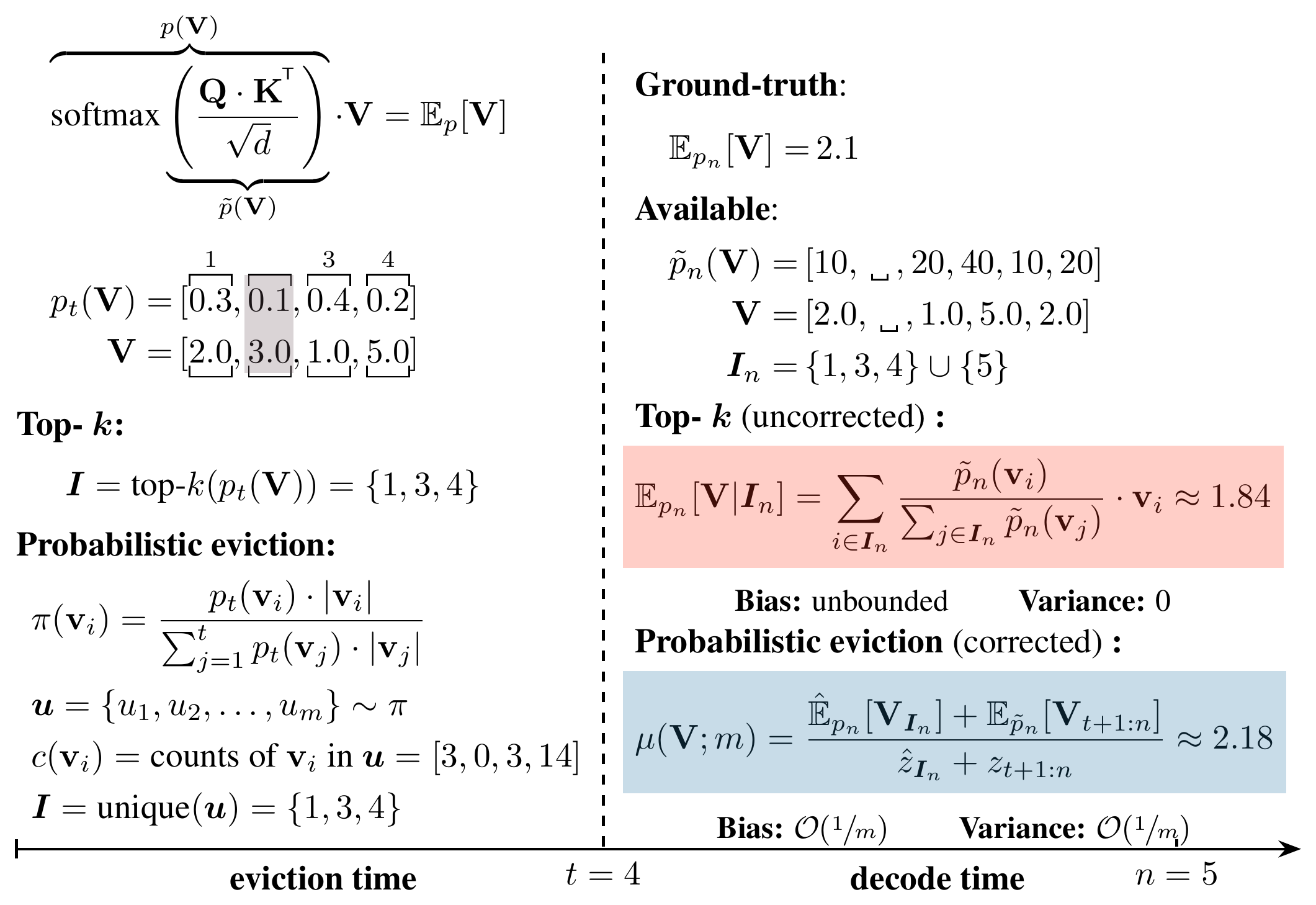
The common approach in KV eviction is to score entries by using the attention weights and values, and then take the top- $k$ entries according to these scores ([6, 8, 7]); this estimator is zero-variance as it is deterministic. However, it can have an arbitrarily large bias. We instead suggest that these scores should be viewed as unnormalized distributions on entries which to evict, allowing us to later reuse them as a proposal distribution to correct for the distortion caused by eviction through self-normalized importance sampling. This is an attractive option because self-normalized importance sampling has reasonable upper bounds on bias and variance ([9, 10]). Figure 1 summarizes our approach.

$**Figure 1:** **Correction can attenuate the effects of eviction at decode time.** Evicting entries deforms the distribution and biases the expectation, as the normalizing constant is altered by the evicted entries. Existing eviction methods deterministically evict the top- $k$ scored entries, which although zero-variance, may have arbitrarily large bias. Probabilistic eviction addresses this unintended deformation through self-normalized importance sampling, whose error is upper bounded by $\mathcal{O} (m^{-1})$, where $m$ is the number of samples.$

In summary, our contributions are as follows:

We show that KV eviction is NP-complete (Section 3);
We formalize KV eviction as an expectation estimation problem and show an asymptotically correct estimator for the decode time expectation with bounded bias and variance (Section 4 and Section 5);
We show the interplay of bias versus variance in this estimator and how existing eviction methods are subsumed by this framework (Section 6 and Appendix D);
We empirically validate our findings by showing that coupling probabilistic eviction and decode time correction is not only competitive at the same compression budget but is more robust across different tasks (Section 7).

2. Preliminaries

Section Summary: This section introduces the paper's notation and reviews core concepts for handling long sequences in transformer attention. It first describes the standard attention computation using query, key, and value matrices, then explains KV caching, which stores prior key and value results so each new token can be generated without recomputing the full sequence. Finally, it covers KV cache eviction, which drops selected cached entries to shrink memory use and speed up inference while aiming to preserve output quality.

We start by briefly introducing notation and reviewing the attention mechanism of [11] as well as the concepts of KV caching and KV eviction. Throughout this paper, we shall denote random variables (RVs) as single upper case letters (e.g. $X, Y, Z$), their values or scalars as single lower case letters (e.g. $x, y, z$), sets as bold letters (e.g. $\bm{X}, \bm{Y}, \bm{Z}$ for RVs or $\bm{x}, \bm{y}, \bm{z}$ for values), and sequences or matrices as bold upright lower and upper case letters respectively (e.g. $\mathbf{x}, \mathbf{y}, \mathbf{z}$ for sequences and vectors, and $\mathbf{X}, \mathbf{Y}, \mathbf{Z}$ for matrices).

Attention. Let $\mathbf{K}, \mathbf{Q}, \mathbf{V}\in\mathbb{R}^{n\times d}$ be the key, query and value embedding matrices for a particular attention head, where $n$ is the token sequence length and $d$ is the embedding dimension. Attention is computed as

$ \mathbf{O}\vcentcolon= \text{softmax}\left(\frac{\mathbf{Q}\cdot\mathbf{K}^{^{\mkern-1.5mu\mathsf{T}}}}{\sqrt{d}}\right)\cdot\mathbf{V},\tag{1} $

where the denominator inside the softmax is often omitted as it is mostly used as a regularizer during training (and here we shall do so as well). This computation ultimately yields a matrix $\mathbf{O}\in\mathbb{R}^{n\times d}$ corresponding to the attention values for each of the $n$ entries. The key, query and value embeddings for the next layer are then computed as a function of $\mathbf{O}$.

KV caching. The intermediate softmax computation is $n\times n$ which can be prohibitively large at longer sequences. Because generation depends only on the next token attention values, it is therefore useful to, instead of fully computing the softmax matrix in Equation 1, compute only the last row of the softmax matrix and cache $\mathbf{K}$ and $\mathbf{V}$ at each attention head

$ \underbrace{\mathbf{o}}{1\times d}\vcentcolon=\overbracket[0.1ex]{\text{softmax}\Big(\underbrace{\mathstrut\mathbf{Q}{-1}}{1\times d}\cdot\underbrace{\mathstrut\mathbf{K}^{^{\mkern-1.5mu\mathsf{T}}}}{d\times n}\Big)}^{1\times n}\cdot\overbracket[0.1ex]{\mathbf{V}}^{n\times d}= \text{softmax}(\overbracket[0.1ex]{[\underbrace{\mathstrut\mathbf{k}i}{1\times d}\cdot\underbrace{\mathstrut\mathbf{q}n}{d\times 1}] _{i=1}^n}^{1\times n})\cdot\overbracket[0.1ex]{\mathbf{V}}^{n\times d};\tag{2} $

where here we annotate matrices and vectors with their dimensions for clarity. The cached keys and values $\mathbf{k}_{1}, \mathbf{k}_2, \dots, \mathbf{k}_n$ and $\mathbf{v}_1, \mathbf{v}_2, \dots, \mathbf{v}_n$ are then reused in the next $n+1$ forward pass.

KV cache eviction. One popular strategy to further speed up computation is to further reduce the softmax computation in Equation 2 to a subset of entries. Let $\bm{I}\subseteq [1..n]$ be the set of indices of which entries to keep, where here we denote $[i..j]$ as the set of positive integers in $[i, j]$. The KV cache evicted attention of an attention head with kept entries $\bm{I}$ is given by

$ \mathbf{o}_{\bm{I}}\vcentcolon= \text{softmax}\left(\left[\mathbf{k}_i\cdot\mathbf{q}_n\right] {i\in\bm{I}}\right)\cdot\mathbf{V}{\bm{I}},\tag{3} $

where $\mathbf{V}_{\bm{I}}$ indicates indexing the rows of $\mathbf{V}$ with $\bm{I}$. The remaining entries not in $\bm{I}$ are evicted from the cache. This is KV cache eviction. The goal in eviction is to thus select an appropriate $\bm{I}$ such that downstream performance is (ideally) unaffected or only slightly impacted. We refer the reader to Appendix A for a discussion on related work.

Now that we understand the setting and the goal of KV (cache) eviction, we are ready to formalize and study KV eviction. We start by showing its hardness.

3. KV Cache Eviction is Hard

Section Summary: The section proves that deciding which entries to drop from a KV cache is fundamentally difficult. It formalizes the eviction task as a decision problem that asks whether a small subset of key-value pairs can reproduce the original attention output within a given error tolerance, then shows this problem is NP-complete by a direct reduction from the classic Partition problem. The authors emphasize that their formulation is actually an easier version of real-world eviction, since it only requires matching attention at the moment of eviction rather than at future decoding steps, yet it remains computationally intractable.

First and foremost we state the problem, its input and output.

########## {caption="Problem 1: KVEviction"}

Input. Matrices $\mathbf{K}, \mathbf{Q}, \mathbf{V}\in\mathbb{Q}^{n\times d}$, error $\varepsilon\in\mathbb{Q}^d$, and compression ratio $r\in(0, 1)$.

Output. Whether there exists a set $\bm{I}\subset[1..n]$ such that $|\bm{I}|=\lfloor n\cdot r\rfloor$ and

$ \left| \text{softmax}\left(\left[\mathbf{k}_i\cdot\mathbf{q}_n\right] {i\in\bm{I}}\right)\cdot\mathbf{V}{\bm{I}}-\text{softmax}\left(\left[\mathbf{k}_i\cdot\mathbf{q}_n\right] _{i=1}^n\right)\cdot\mathbf{V}\right|\leq\varepsilon.\tag{4} $

Our reduction is from the $\textsc{Partition}$ problem.

########## {caption="Problem 2: Partition"}

Input. A sequence of $n$ integers $\mathbf{v}=(v_1, v_2, \dots, v_n)$.

Output. Whether there exists a set $\bm{I}\subset[1..n]$ such that $|\bm{I}|=\lfloor\frac{n}{2}\rfloor$ and

$ \sum_{v\in\mathbf{v}{\bm{I}}}v=\sum{u\in\mathbf{v}_{\overline{\bm{I}}}}u, $

where we here denote $\mathbf{v}_{\overline{\bm{I}}}$ to mean the values in $\mathbf{v}$ not indexed by $\bm{I}$.

########## {caption="Theorem"}

$\textsc{KVEviction}$ is NP-complete.

Proof sketch: Without loss of generality, assume $n$ to be even; set $d=1$, $r=\frac{1}{2}$, $\varepsilon=0$ and $\mathbf{K}=\mathbf{Q}=\mathbf{1}{n\times d}$, where here we denote $\mathbf{1}{m\times n}$ as the all-ones matrix in $\mathbb{Q}^{m\times n}$. Hardness follows immediately by simply reducing the expression in Equation 4, which then yields the $\textsc{Partition}$ problem, which is NP-hard. If one can solve $\textsc{KVEviction}$ for this case, then one can solve any instance of $\textsc{Partition}$, meaning $\textsc{KVEviction}$ is at least as hard as $\textsc{Partition}$. Membership in NP requires some care to ensure that the softmax is computable in $\mathbb{Q}$; still, this operation can be approximated according to the precision of $\varepsilon$. The full reduction and membership proof is stated in Appendix B.

The attentive reader might recognize that $\textsc{KVEviction}$ is in fact an easier problem compared to real-world KV eviction. In KV eviction, the goal is to preserve the attention head values at decode time—i.e. the future time steps after entries have been evicted and are no longer available to compute. Our results show that even preserving the attention head values at eviction time—when we have access to all the ground-truth values—is hard.

With this in mind, our goal now is to exploit the structure of $\textsc{KVEviction}$ in order to find principled KV eviction approximations. We do so by a probabilistic interpretation of KV eviction, showing that through this lens we obtain a richer space of eviction strategies.

4. A Probabilistic Interpretation of KV Cache Eviction

Section Summary: This section frames attention as computing expectations of value vectors under categorical distributions induced by the softmax over keys, so that KV cache eviction amounts to selecting a subset of entries whose weighted sum will approximate those expectations. Standard top-k eviction methods based on importance scores are interpreted as zero-variance but biased estimators that remain skewed even at the moment of eviction. In contrast, sampling from the attention distribution (or any suitable proposal) yields an unbiased estimator at eviction time, though future tokens will still require importance-sampling corrections to account for the removed entries.

A natural yet crucial observation is that the softmax matrix in Equation 1 induces $n$ distributions (one for each row of the matrix) over the $n$ entries represented by each column. The resulting attention value for an attention head is thus a matrix containing the dot product of these probabilities with the values $\mathbf{V}$. This amounts to computing the expectation of $\mathbf{V}$ under a distribution $p_i(\mathbf{V})$ parameterized by $\mathbf{q}_i$ and $\mathbf{K}$. It is important to note that this distribution is not over the space of values $\mathbb{R}^{n\times d}$, but rather is a categorical distribution over the $n$ entries (i.e. indices) that map to $\mathbf{V}$.

$ \text{softmax}\left(\mathbf{Q}\cdot\mathbf{K}^{^{\mkern-1.5mu\mathsf{T}}}\right)\cdot\mathbf{V}=\big[\overbrace{\text{softmax}\left(\mathbf{q}_i\cdot\mathbf{K}^{^{\mkern-1.5mu\mathsf{T}}}\right)}^{p_i(\mathbf{V})}\big] {i=1}^n\cdot\mathbf{V}=\left[\sum{j=1}^n p_i(\mathbf{V}=\mathbf{v}_j)\cdot\mathbf{v}_j\right] {i=1}^n=\left[\mathbb{E}{p_i}\left[\mathbf{V}\right]\right] _{i=1}^n\tag{5} $

In short, attention is nothing more than computing expectations. When using a KV cache, this further reduces to simply computing a single expectation of a $d$-dimensional vector on the last row. This provides an interesting framework for KV eviction: Each entry now has a clear distribution associated to it and can—within the setting of KV eviction—be interpreted as the probability distribution of keeping that entry. The goal of KV eviction then becomes to find a subset $\bm{I}$ that estimates future expectations with least bias and variance.

Interestingly, existing eviction methods usually base their eviction decision on computing some score, either from $p_n(\mathbf{V})$ or $\mathbf{V}$, and then taking the top- $k$ highest scored entries to keep ([12, 6, 8]). This is a zero-variance yet clearly biased estimator (and in fact unboundedly biased), skewing the expectation even at eviction time.

A simple and easy solution to achieve unbiasedness at eviction time is to select $\bm{I}$ according to samples from $p_n(\mathbf{V})$. For a given number of samples $m$ taken with replacement from $p_n(\mathbf{V})$, $\bm{I}$ can be chosen as the collection of unique entries in this set of samples. This provides an unbiased eviction estimator at eviction time. In fact, one can use any proposal distribution $\pi$ in order to probabilistically evict from the cache and later adjust the expectation computation with importance sampling.

The choice of which proposal to use is open to the user as long as its support covers all entries. In fact, existing top- $k$ score KV eviction methods are easily subsumed in this framework by interpreting these scores as an unnormalized proposal distribution $\tilde{\pi}$ (Appendix D). Indeed, given a score eviction strategy, there exists an infinite number of proposal distributions whose top- $k$ also correspond to the same top- $k$ of that strategy. Top- $k$ eviction corresponds to computing the expectation conditioned on the $k$-maximum a posteriori (MAP) states as a proxy for the eviction time expectation, while probabilistic eviction—i.e. sampling from $\pi$ and choosing all entries which have been sampled at least once—estimates the expectation through importance sampling.

So far we have seen that top- $k$ is biased even at eviction time, while probabilistic eviction emerges as an unbiased eviction time alternative. However, this discussion ignores the future; the distribution at later steps will have missing probabilities which can potentially cause further error to future expectations. Thus, a natural question to ask ourselves is:

########## {caption="Goal"}

If we evict at time step $t$, can we correct CrefnameequationEq.Eqs. Equation 3 for the missing entries at time steps

gt;t$?

As we shall see in the next sections, we can make use of the proposal distribution and its samples used in probabilistic eviction to correct decoding.

5. Correcting for Eviction

Section Summary: At eviction time t, standard attention ignores any discarded KV entries when computing later decode steps, which distorts the original probability distribution by rescaling the remaining weights and lets small errors compound through subsequent layers. The method counters this distortion by applying self-normalized importance sampling: the proposal distribution and sample counts recorded at eviction are reused at each future step to reweight the kept entries so their contribution matches the true conditional expectation. The overall expectation is further split into a pre-eviction term (approximated via importance sampling) and a post-eviction term (computed exactly), then combined with weights that reflect the renormalized probability mass on each side of the eviction boundary.

Given a sequence of length $t$, the task of KV eviction is usually to perform eviction on this sequence—i.e. at time step $t$ —and then generate new tokens at future time steps $n>t$. We shall call time step $t$ eviction time and any time step after that decode time. While at eviction time we have access to all previous distributions $\left[p_i(\mathbf{V})\right] {i=1}^t$, at decode time $n>t$ we only have access to the kept entries of $p_n(\mathbf{V})$ (as well as cached keys $\mathbf{K}{\bm{I}}$ and values $\mathbf{V}_{\bm{I}}$). The usual treatment in the literature is to ignore missing entries and compute attention as usual. However, this severely changes the distribution, as this amounts to conditioning the distribution to restricting its support to only kept entries

$ \text{softmax}\left(\left[\mathbf{k}_i\cdot\mathbf{q}_n\right] _{i\in\bm{I}t^{n}}\right)\cdot\mathbf{V}{\bm{I}_t^n} =\left[\frac{p_n(\mathbf{v}_i)\cdot \llbracket i\in\bm{I}t^n \rrbracket}{\sum{j\in\bm{I}_t^n} p_n(\mathbf{v}_j)}\right] {i=1}^n\cdot\mathbf{V}{\bm{I}_t^n} =p_n\left(\mathbf{V}|\bm{I}t^n\right)\cdot\mathbf{V}{\bm{I}t^n} =\mathbb{E}{p_n}\left[\mathbf{V}|\bm{I}_t^n\right],\tag{6} $

where $\bm{I}_t^n \vcentcolon=\bm{I}\cup[t+1..n]$ —i.e. all the kept entries and all the entries generated after eviction time—, and $\llbracket\cdot \rrbracket$ denotes the Iverson bracket. This means that the contribution of each entry will be excessively boosted or diminished by the normalizing constant proportionally to the probability mass evicted. Furthermore, because $\mathbf{K}$, $\mathbf{V}$ and $\mathbf{Q}$ are all computed as a function of the attention values of the previous layer, any error—even if small—propagates and is amplified to all following layers and future generations.

To correct for this, we utilize self-normalized importance sampling to adjust the probabilities at decode time ([13, 14, 9]). This requires we exploit the probabilistic interpretation introduced in Section 4. In summary, given a proposal distribution $\pi$ at eviction time $t$, we sample entries from $\pi$, record their counts, and evict any entries that have not been sampled. At decode time, we then use $\pi$ and the sampled counts to correct for eviction through self-normalized importance sampling. We now describe this process in detail and show that the corrected expectation estimate is asymptotically correct. To do so, let us first properly define the tools we are going to use.

########## {caption="Definition 3: Self-normalized importance sampling"}

Let $\tilde{p}(X)$ be an unnormalized probability distribution over an RV $X$ that can take $n$ values, $p$ its normalized distribution, and $\pi(X)$ a proposal distribution also over $X$. Given $m$ samples from $\pi$, the function $c(x)$ maps the value $x$ to the number of times $x$ has been sampled from $\pi$. The self-normalized importance sampling estimator for the expectation $\mathbb{E}_p\left[X\right]$ is

$ \hat{\mu}(X;\tilde{p}, \pi, m)\vcentcolon=\frac{1}{m}\sum_{i=1}^n \frac{c(x_i)\frac{\tilde{p}(x_i)}{\pi(x_i)}}{\frac{1}{m}\sum_{j=1}^n c(x_j)\frac{\tilde{p}(x_j)}{\pi(x_j)}}x_i\stackrel{m\to\infty}{=}\mathbb{E}_\pi\left[\frac{p(X)}{\pi(X)}\cdot X\right]=\mathbb{E}_p\left[X\right].\tag{7} $

Our goal is to estimate the expectation at decode time $n$. In order to do so, we slightly massage the expectation into a more appealing expression

$ \begin{aligned} \mathbb{E}{p_n}\left[\mathbf{V}\right] &=\sum{i=1}^n p_n(\mathbf{v}i)\cdot\mathbf{v}i =\frac{\sum{i=1}^t \tilde{p}n(\mathbf{v}i)\cdot\mathbf{v}i + \sum{i=t+1}^n \tilde{p}n(\mathbf{v}i)\cdot\mathbf{v}i}{\sum{j=1}^n \tilde{p}n(\mathbf{v}i)}\nonumber\ &=\frac{\mathbb{E}{\tilde{p}n}\left[\mathbf{V}{1:t}\right] + \mathbb{E}{\tilde{p}n}\left[\mathbf{V}{t+1:n}\right]}{z} =\mathbb{E}{p_n^{(1:t)}}\left[\mathbf{V}\right]\cdot\frac{z{1:t}}{z{1:t}+z{t+1:n}}+\mathbb{E}{p_n^{(t+1:n)}}\left[\mathbf{V}\right]\cdot\frac{z_{t+1:n}}{z_{1:t}+z_{t+1:n}}\nonumber\ &=\mathbb{E}{p_n^{(1:t)}}[\mathbf{V}]\cdot p(T\leq t)+\mathbb{E}{p_n^{(t+1:n)}}[\mathbf{V}]\cdot p(T>t). \end{aligned}\tag{8} $

We use the superscript to denote the distribution restricted to the support specified by the interval and then renormalized accordingly $p^{(i:k)}(X)\vcentcolon=\left[\frac{p(x_j)}{\sum_{l=i}^k p(x_l)}\right] {j=i}^k$. Similarly, $\mathbf{V}{i:k}$ is used to denote a restriction on the values of $\mathbf{V}$ to ${\mathbf{v}j}{j=i}^k$. Lastly, we use $z$ to denote the normalizing constant and correspondingly $z_{i:k}\vcentcolon=\sum_{j=i}^k\tilde{p}_n(\mathbf{v}_j)$ to mean the normalizing constant for that interval.

The final expression in Equation 8 tells us that we may decompose the expectation into two local expectations: before and after eviction, as long as we weigh them appropriately according to $p(T\leq t)$ and $p(T>t)$. The local expectation after eviction $\mathbb{E}_{p_n^{(t+1:n)}}[\mathbf{V}]$ can be computed exactly: all entries are available. However, the local expectation before eviction contains missing entries and thus needs to be approximated. Indeed, both $p(T\leq t)$ and $p(T>t)$ also need to be approximated as their denominator is the normalizing constant $z$. To do so, we define the following estimator.

########## {caption="Definition 4: Attention estimator"}

The estimator for corrected attention is given by

$ \mu_n(\mathbf{V};m)\vcentcolon= \hat{\mu}(\mathbf{V};\tilde{p}n^{(1:t)}, \pi, m)\cdot p(T\leq t)+\mathbb{E}{p_n^{(t+1:n)}}[\mathbf{V}]\cdot p(T>t),\tag{9} $

where $\hat{\mu}$ is a self-normalized importance sampling estimator that uses the unnormalized distribution $\tilde{p}n^{(1:t)}$ as the target distribution and $\pi$ as the proposal. The probabilities $p(T\leq t)$ and $p(T>t)$ are approximated by aggregating the importance weights from $\mu_n$: $\hat{z}{1:t}=\frac{1}{m}\sum_{j=1}^t c(\mathbf{v}_j)\frac{\tilde{p}_n(\mathbf{v}_j)}{\pi(\mathbf{v}_j)}$.

This estimator is asymptotically correct w.r.t. the desired expectation estimand (see Appendix C).

########## {caption="Proposition"}

If $\text{supp}(\pi)\supseteq \text{supp}(p_n)$, then $\lim_{m\to\infty}\mu_n(\mathbf{V};m)=\mathbb{E}_{p_n}[\mathbf{V}]$.

Require: KV cache $\mathbf{K},\mathbf{V}\in\mathbb{R}^{n\times d}$, sample counts $[c(\mathbf{v}_i)]_{i\in\bm{I}}$, proposal $\pi$, current query $\mathbf{q}_n\in\mathbb{R}^d$.
Ensure: Corrected attention $\mathbf{o}\in\mathbb{R}^d$
$\tilde{p}_n\gets\exp\left(\mathbf{q}_n\cdot\mathbf{K}^{^{\mkern-1.5mu\mathsf{T}}}\right)$ // Unnormalized probabilities of non-evicted entries
$w_i\gets c(\mathbf{v}_i)/(m\cdot \pi(\mathbf{v}_i))$, $\forall i\in[1..t]$ // Weights to be applied to the unnormalized probabilities
$\hat{z}_{1:t}\gets\sum_{i=1}^t w_i\cdot\tilde{p}_n(\mathbf{v}_i)$ // Normalizing constant for the eviction time entries
$z_{t+1:n}\gets\sum_{i=t+1}^n \tilde{p}_n(\mathbf{v}_i)$ // Normalizing constant for the decode time entries
$\hat{\mu}_{1:t}\gets\sum_{i=1}^t w_i\cdot\tilde{p}_n(\mathbf{v}_i)\cdot\mathbf{v}_i$ // Estimated unnormalized expectation for eviction time
$\mu_{t+1:n}\gets\sum_{i=t+1}^n\tilde{p}_n(\mathbf{v}_i)\cdot\mathbf{v}_i$ // Exact unnormalized expectation for decode time
$\mathbf{o}\gets\frac{\hat{\mu}_{1:t}+\mu_{t+1:n}}{\hat{z}_{1:t}+z_{t+1:n}}$ // Corrected attention value after normalization
return $\mathbf{o}$

Note that although $\mu_n(\mathbf{V};m)$ is still biased for a fixed number of samples $m$, this only comes from the self-normalized importance sampling estimator, which has both bias and (mean squared) error upper bounded by $O(\frac{1}{m})$ ([10], Theorem 2.1). In other words, more samples reduce this error significantly. This bias can be further reduced by applying any bias-reducing method for self-normalized importance sampling to $\mu_n(\mathbf{V};m)$ ([15]). In contrast to this bound, existing KV eviction methods deterministically keep the top- $k$ entries according to some score on either $p_t(\mathbf{V})$ or $\mathbf{V}$ and thus are zero-variance yet unboundedly biased ([6, 8, 7]).

Equipped with Definition 4 and, we can now explicitly construct the correction algorithm for decode time. Algorithm 1 shows how to compute the corrected attention value for a given attention head. Note that here we simplify the algorithm and notation due to space constraints, but one must be careful when computing the corrected probabilities: an entry $i$ is evicted iff $c(\mathbf{v}_i)=0$, meaning that $\tilde{p}_n(\mathbf{v}_i)$ will be undefined. Any entry which is missing due to eviction should be properly ignored in the computation.

Ultimately, the pipeline is as follows: at eviction time $t$, (1) construct a proposal distribution $\pi^{(h)}$ for each attention head $h$, and (2) sample counts $[c^{(h)}(\mathbf{v}_i)] _{i=1}^t$. At decode time $n$, (3) compute attention following Algorithm 1.

Some attention has to be paid when dealing with grouped query attention ([16]): Because every attention head in a group $\bm{G}={h_1, h_2, \dots, h_g}$ shares the same $\mathbf{K}$ and $\mathbf{V}$ caches, ingroup eviction and correction have to be consistent. To do so, we use one proposal $\pi^{(\bm{G})}$ per group, ensuring that the support of $\pi^{(\bm{G})}$ contains the support of every attention head distribution by constructing a mixture of each head proposal $\pi^{(\bm{G})}(\mathbf{v}i)\vcentcolon=\sum{j=1}^g\alpha_j\cdot\pi^{(h_j)}(\mathbf{v}_i)$, where every $\alpha_j\in\Delta^{g-1}$ comes from the $(g-1)$-simplex.

So far, our contributions have been either theoretical or philosophical. In the next section, we empirically validate probabilistic eviction and correction, studying the role of bias and variance in KV eviction.

6. Bias vs Variance

Section Summary: The section explains that KV cache eviction involves a practical trade-off between bias and variance when using importance sampling to correct for dropped tokens. Introducing a temperature parameter on the importance weights allows variance to be deliberately lowered at the expense of added bias, which reduces overall error in attention values once the number of retained samples becomes very small. Experiments on models like Llama3 show that bias contributes far more to attention inaccuracy than variance does, favoring eviction strategies that keep bias low rather than forcing variance to zero.

$**Figure 2:** **KV eviction is a game of trading bias for variance and vice versa.** The plot shows mean absolute error ($y$-axis) of the attention values for the first token after an evicted prompt on **Llama3** averaged across all heads (see Appendix E for details) for different compression ratios ($x$-axis). Bias and variance are low at lower $r$, since $m$ (number of samples) is high. As $r$ increases, $m$ decreases, causing variance to increase more than bias. Higher importance weight temperatures $\tau$ decrease the variance, causing the error to decrease at extremely high $r$ 's.$

Although bias and variance share the same asymptotic upper bounds in self-normalized importance sampling, in practice they may present distinct behaviors ([10]). In this section, we show that by decreasing the variance at the cost of more bias, we are able to achieve lower error under certain conditions. To do so, we introduce a temperature scaling parameter $\tau\in[0, \infty)$ to the importance weights. We then replace 4 in Algorithm 1 with

$ w_i\gets \exp\left(\frac{1}{\tau}\cdot\log\left(\frac{c(\mathbf{v}_i)}{m\cdot\pi(\mathbf{v}_i)}\right)\right), \forall i\in[1..t].\tag{10} $

When $\tau=1$, Equation 10 reduces to the same expression as 4; when $\tau\to\infty$, it is equivalent to not applying correction since $w_i$ approaches $1$. This reduces variance, since the stochasticity comes from the samples of the proposal distribution, which can be amplified by the correction. By suppressing correction, variance is reduced. Temperatures below $1$ cause Algorithm 1 to give more importance (i.e. probability mass) to entries in $[1..t]$ compared to decode time entries.

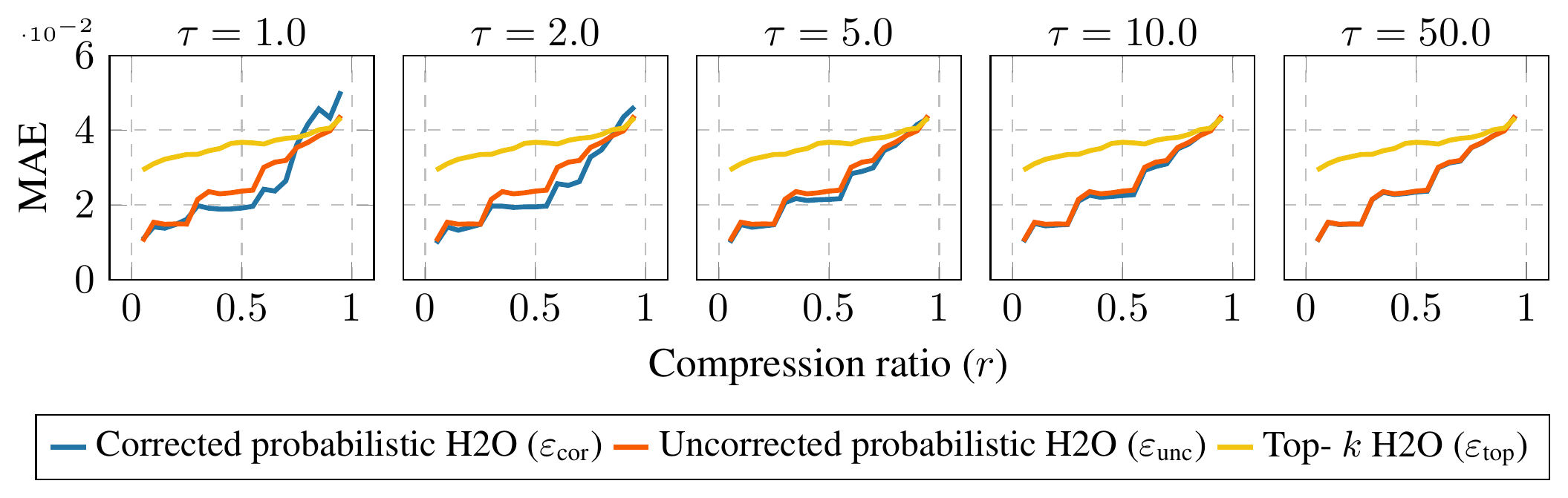
Our goal is to show the impact of bias and variance in terms of the mean absolute error (MAE) between the estimated expectation and the ground-truth expectation. Given a prompt $\mathbf{x}$ and a first response token $y$, we compute the KV cache $(\mathbf{K}, \mathbf{V})$ on $\mathbf{x}$ and apply probabilistic eviction using a proposal $\pi$ constructed from the scores of the H2O eviction method ([8]) (see Appendix D for details). This results in an evicted KV cache $(\mathbf{K}{\bm{I}}, \mathbf{V}{\bm{I}})$. We then compute the average error between the uncorrected $\mathbf{o}{\bm{I}}$ and ground-truth $\mathbf{o}$ attention values $\varepsilon\text{unc}$, and between the corrected $\mu_n(\mathbf{V};m)$ and ground-truth attention values $\varepsilon_\text{cor}$ across all $h$ attention heads

$ \varepsilon_{\text{unc}}\vcentcolon=\frac{1}{h}\cdot\sum_{i=1}^h\left|\mathbf{o}^{(i)}-\mathbf{o}{\bm{I}}^{(i)}\right|, \quad\varepsilon{\text{cor}}\vcentcolon=\frac{1}{h}\cdot\sum_{i=1}^h\left|\mathbf{o}^{(i)}-\mu_n^{(i)}(\mathbf{V};m)\right|.\tag{11} $

Finally, we compute the error $\varepsilon_\text{top}$ between the ground-truth and H2O's estimation of the attention.

In order to provide a fair comparison of $\varepsilon_\text{cor}$ and $\varepsilon_\text{unc}$ against $\varepsilon_\text{top}$, we constrain the compression ratio to be the same for every attention head. To do so, for each attention head, we select a number of samples that achieves, on average, the desired compression ratio. In Appendix F, we discuss how this problem relates to the classical coupon collector problem and provide a tractable approximation with negligible error in practice.

Figure 2 shows the average errors across compression ratios $r\in[0, 1]$ and temperatures $\tau\in{1, 2, 5, 10, 50}$ for Llama3**.2-3B** ([17]); prompt $\mathbf{x}$ and first token $y$ are described in Appendix E. Lower compression ratio $r$ implies a higher number of samples $m$. When $m$ is high, bias and variance are low; when $m$ is extremely low, variance is very high, causing $\varepsilon_\text{cor}$ to be much higher than $\varepsilon_\text{unc}$. This is where temperature scaling provides an improvement by reducing the variance at a cost to bias. As the middle ranges of $r$ show, increasing bias when variance is already low harms estimation quality. The $\varepsilon_\text{unc}$ curve does not match with $\varepsilon_\text{top}$ because eviction is done stochastically, while H2O greedily evicts the top- $k$. This shows that even probabilistic eviction by itself allows for less error. As $r$ approaches one, the probabilistic choices all collapse to the top- $k$, which is when $\varepsilon_\text{unc}$ and $\varepsilon_\text{top}$ meet.

In this section, we showed how correction allows for a trade-off between bias and variance. However, in practice bias plays a much larger role in attention error. This motivates the shift from low-variance high-bias to higher-variance low-bias estimators. As we shall see in the next section, corrected probabilistic eviction tends to produce more robust estimators compared to existing zero-variance unbounded bias KV eviction strategies due to reduced bias.

7. Robustness

Section Summary: The section demonstrates that standard KV cache eviction methods relying on fixed heuristics often fail dramatically on specific tasks due to unmitigated bias. By testing probabilistic eviction strategies against established approaches like StreamingLLM, SnapKV, TOVA, and H2O on Llama and Qwen models using LongBench and RULER, the authors show that their sampling-based methods deliver competitive overall accuracy while proving far more consistent across diverse tasks. A win-score metric that ranks methods per example reveals that variance-reduced probabilistic proposals, especially those incorporating a harmonic prior, avoid the catastrophic per-task drops seen in deterministic baselines and remain robust even at higher compression ratios.

In this section, we show that zero-variance estimators suffer from a heuristic misalignment, where the fixed bias introduced by these heuristics can cause catastrophic failures in certain tasks. To do so, we compare probabilistic eviction against four popular existing KV eviction methods: StreamingLLM ([5]), SnapKV ([6]), TOVA ([7]) and H2O ([8]). All of these methods are implemented in KVPress, which we use for evaluation and our own implementation ([18]). We evaluate Llama3**.2-3B** ([17]) and Qwen3**-4B** ([19]) on two standard KV eviction benchmark datasets: LongBench ([20]) and RULER ([21]). Due to compute constraints, we evaluate RULER on a subset of 130 examples and on all instances of the HotpotQA, QASPER and TriviaQA splits of LongBench whose context prompt is shorter than 3000 tokens.

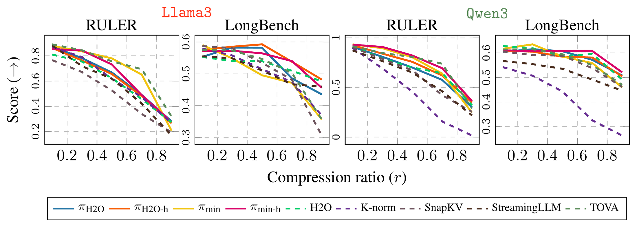
**Figure 3:** **Probabilistic eviction achieves competitive performance.** Probabilistic eviction with correction performs best at lower to middle ranges, when there are enough samples to achieve a lower variance and bias. Solid lines show our approach, dashed lines show existing eviction methods.

To evaluate probabilistic eviction, we propose four different proposal distributions: $\pi_{\text{min}}$, $\pi_{\text{min-h}}$, $\pi_{\text{H2O}}$ and $\pi_{\text{H2O-h}}$ which we formally define in Appendix H and provide proper probabilistic semantics. Intuitively, $\pi_{\text{min}}$ computes the minimum variance proposal distribution for the last query at eviction time $t$, $\pi_{\text{H2O}}$ computes a probabilistic version of H2O where scores are normalized and used as the proposal distribution, $\pi_{\text{min-h}}$ computes the minimum-variance proposal for a distribution where all previous time steps are marginalized and weighted by a harmonic prior $h_j$, and $\pi_{\text{H2O-h}}$ computes H2O with a harmonic prior $h_j$.

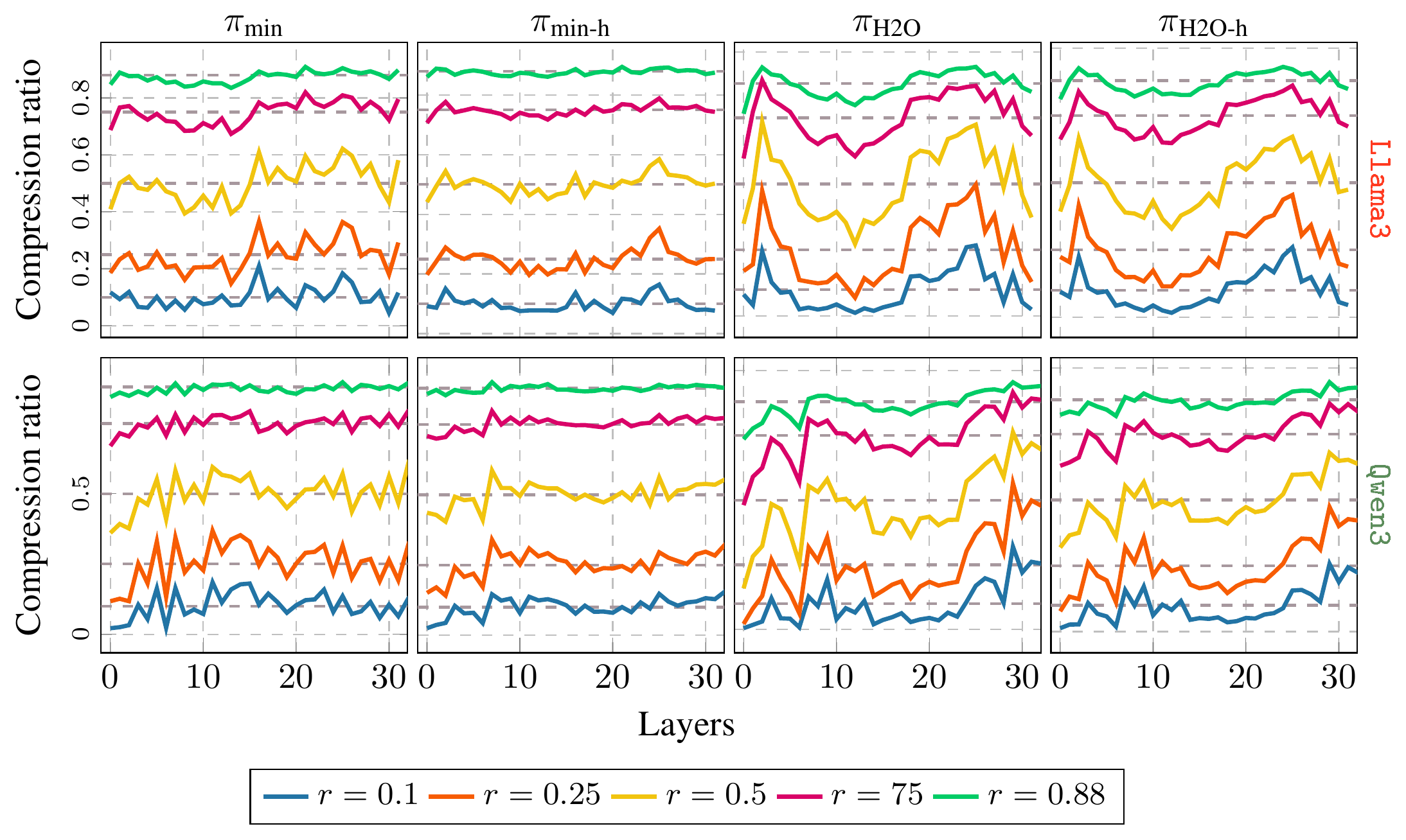
In these experiments, we constrain the compression ratio at the global level: given a compression ratio $r$, we choose a number of samples $m$ such that, on average, the aggregated compression ratio of all KV caches is $r$. This is achieved by a similar mechanism to the one for locally constraining each attention head to a specific compression ratio. Appendix F.1 shows how this can be done and Appendix F.2 provides empirical evidence that the error between the achieved compression ratio and target compression ratio is, in practice, insignificant. Although the overall compression ratio is fixed, every attention head will adaptively choose a suitable compression ratio depending on its distribution. This allows for attention heads that require a lower compression ratio to automatically consume the budget of heads that do not. Interestingly, this results in compression ratios that follow a pattern of lower compression at lower layers, and higher at higher layers (see Appendix I.3 and Figure 9). This is in agreement with the findings of [22], which suggest that allocating more budget to lower layers and less to higher is preferable.

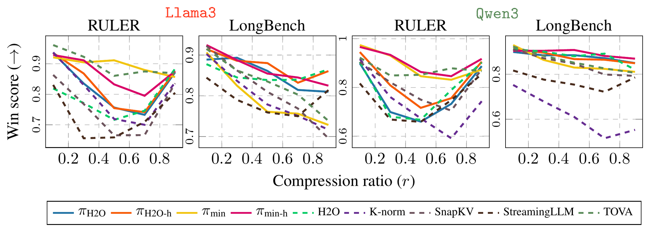
$**Figure 4:** **Probabilistic eviction can make eviction more robust for different tasks.** Win score values for four proposals ($\pi_{\text{H2O}}, \pi_{\text{H2O-h}}, \pi_{\text{min}}, \pi_{\text{min-h}}$) and five top- $k$ estimators (H2O, K-norm, SnapKV, StreamingLLM, TOVA). $\pi_{\text{min-h}}$ achieves best ranking across datasets and models, showing more robustness when minimizing variance and lowering bias.$

Figure 3 shows the average total score in LongBench and RULER for the four previously mentioned proposals and five top- $k$ existing eviction methods. This is computed by averaging the score at each split, weighing them by the fraction of examples in that split and then adding all of these weighted scores together. The average score of each split is given by a scorer function suited to that split $f_{\text{split}}:\mathcal{L}^\ast\to[0, 1]$ that takes in the text generated by the (KV evicted) LLM and attributes a number in $[0, 1]$. For example, HotpotQA uses F1 as the scorer function, while the NIAH (needle-in-a-haystack) split of RULER uses exact string matching. Results show that probabilistic eviction and correction achieve better performance or are at least as competitive as the state-of-the-art.

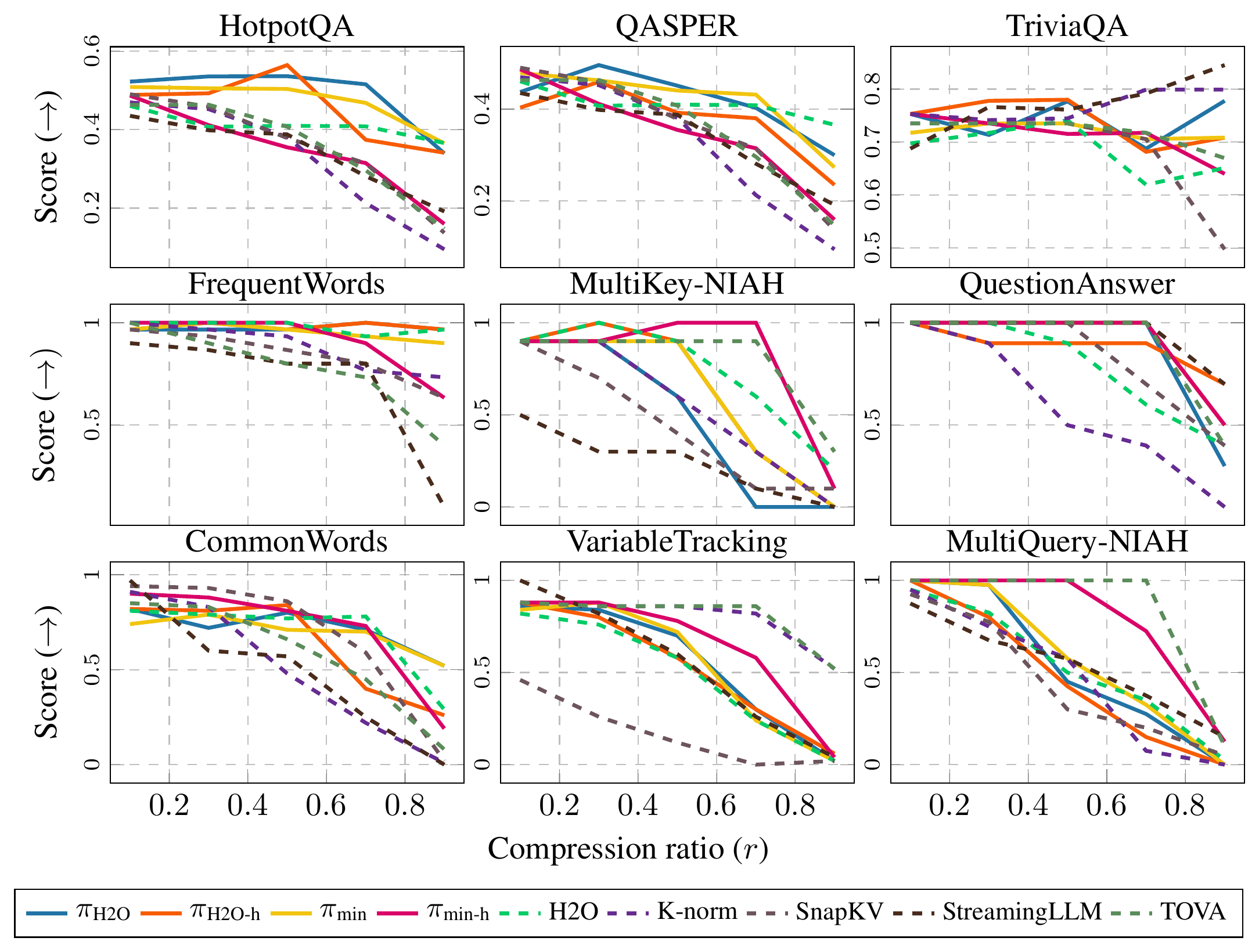
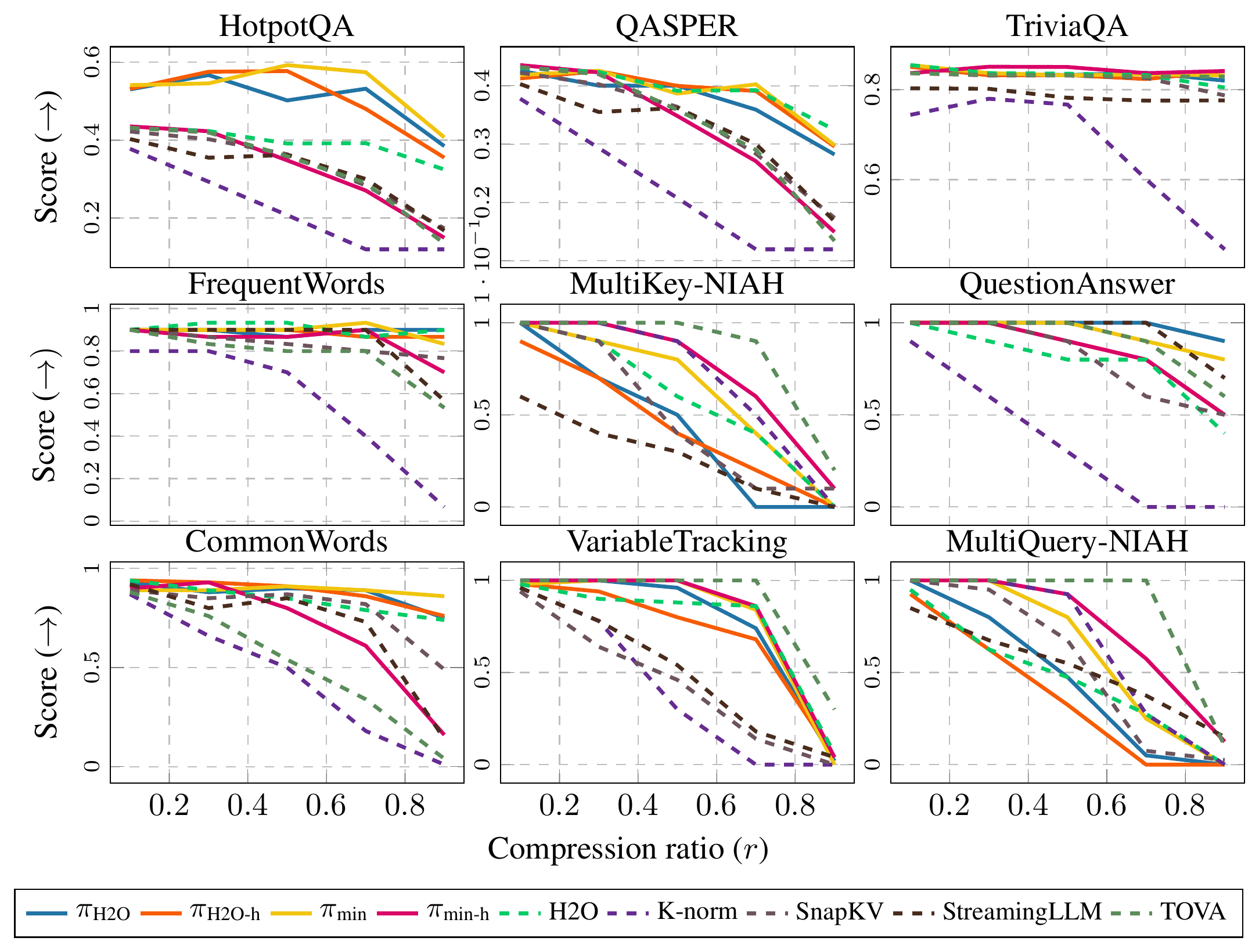
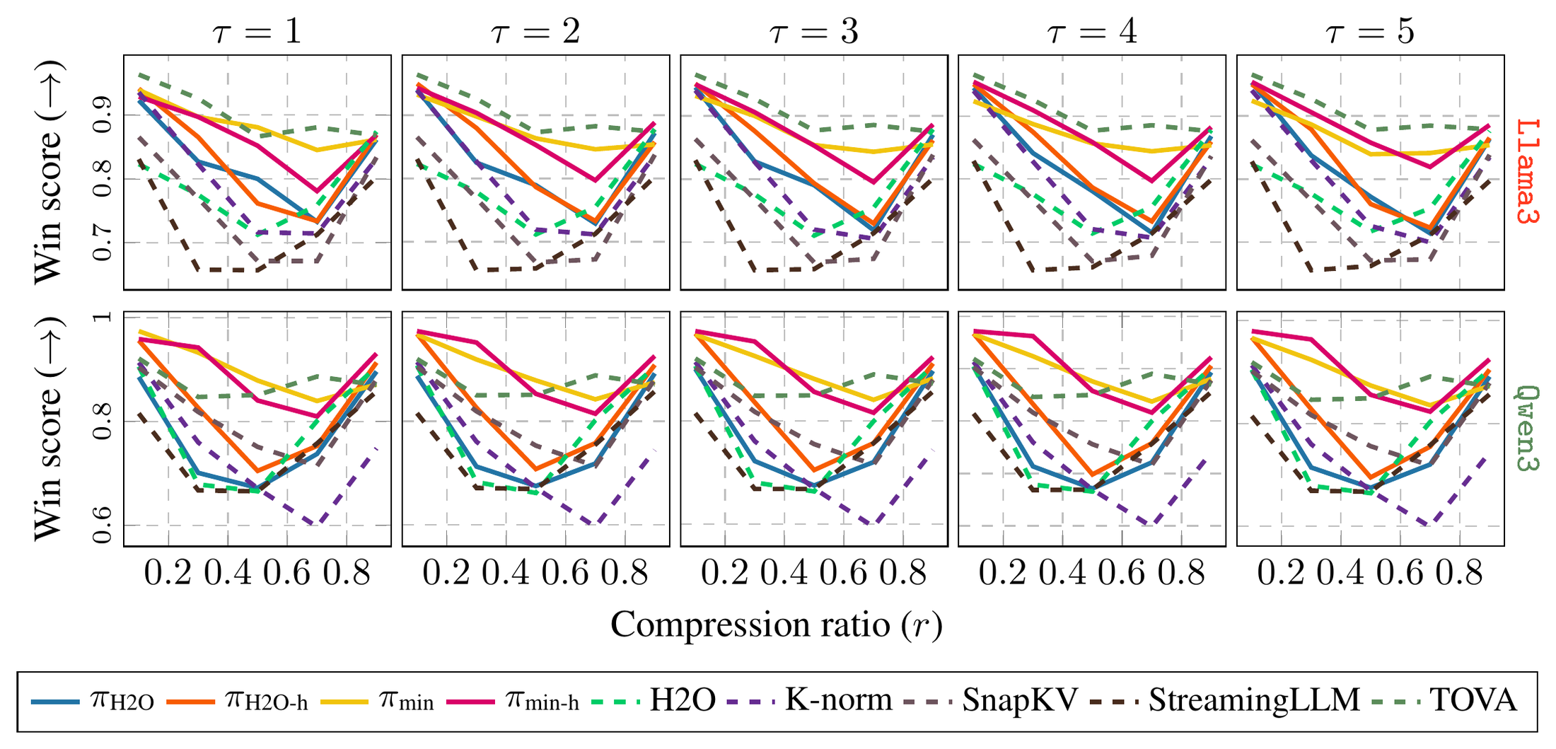
Because these average total scores aggregate over many tasks, they can hide the behavior of eviction methods for certain tasks. For example, on Llama3 StreamingLLM ranks first on the QuestionAnswer split, yet dead last in MultiKey-NIAH (see Figure 5). Similarly, on Qwen3 K-norm is consistently in the top-3 on the MultiKey-NIAH split, yet last in CommonWords (see Figure 6). To account for these catastrophic failures, we measure the pairwise win scores of each method. Specifically, we assign a rank from 0 to $n - 1$ to each method based on how well it performs compared to the other $n - 1$ methods. The method with the lowest score gets a rank of 0, while the method with the highest score gets a rank of $n - 1$. If multiple methods achieve the same score, they are all given the rank corresponding to a win against the other tied methods. Ranking is repeated for all the examples in the task, after which the ranks are normalized by the number of examples in the task to ensure all tasks contribute equally. We refer to the normalized average rank across tasks as the win score.

Figure 4 shows the win score for each proposal and eviction method. Notably, $\pi_{\text{min-h}}$ consistently ranks at the top, showing that it is most robust compared to other methods. Probabilistic eviction tends to do better at low to middle ranges, as there are enough samples to decrease the bias and variance. However, even at higher compression it performs competitively against other eviction methods. Note that when the compression ratio is extremely high (i.e. close to 1.0), all methods do equally poorly, as most of the prompt has been evicted. This is shown as most, if not all, curves increasing in Figure 4, as ties are also rewarded in this scoring.

8. Conclusion

Section Summary: This paper set out to better understand the challenge of deciding what information to remove from an AI model's memory cache when space runs low. The authors showed that the problem is computationally very hard and reframed it as a statistical task of estimating future needs with limited bias and error. They introduced a new sampling-based method that matches the performance of current techniques while proving more reliable across tasks, and they called for closer links between statistics research and AI memory management.

The goal of this paper was to formalize KV cache eviction and in doing so find principled KV eviction estimators. As a result, we showed that KV eviction is NP-complete, and revealed that through a probabilistic interpretation KV eviction is nothing more than an expectation estimation problem. In our quest to characterize this, we found that existing KV eviction methods are zero-variance yet unbounded bias estimators and that a good KV eviction strategy should reduce bias and variance in order to best approximate future expectations. To this end, we proposed a self-normalized importance sampling estimator with reasonable upper bounds on both bias and variance. We then empirically showed that this class of estimators achieves competitive performance against state-of-the-art eviction methods yet are more robust at different tasks. This paper opens up an exciting and promising avenue to developing new KV eviction estimators. We hope that framing KV eviction as an estimation problem and connecting the field of statistical methods with KV cache eviction generates fruitful new research not only within KV eviction but also across other KV cache compression techniques.

Appendix

Section Summary: The appendix reviews prior research on KV cache eviction techniques for accelerating large language model inference, categorizing them by approach and noting that the distortion effects of eviction have received little direct attention. It then establishes that the core KV eviction problem is NP-complete via a reduction from the partition problem, followed by a proof that a proposed sampling-based estimator converges in the limit to the true attention-weighted expectation. The section concludes by showing how conventional score-based eviction strategies can be interpreted as special cases of probabilistic eviction policies.

A. Related Work

KV eviction has received significant interest for the purpose of speeding up inference in large language models. Following the taxonomy given by [23], we categorize KV eviction methods as position-based, attention-based, embedding-based, and hybrid. The most notable examples of each respectively are StreamingLLM ([5]), TOVA ([7]), K-norm ([12]), and SnapKV ([6]). All these methods can be framed as top- $k$ score eviction methods with zero variance and unbounded bias. The problem of correcting for the distortion caused by eviction has not been, as far as we know, properly addressed, although it has been recognized in the literature: [8] acknowledge the issue in passing, while in contemporary work, [3] identify this problem but only as a motivation for KV cache compaction, a more compute-intensive strategy for KV cache compression. The probabilistic interpretation of attention as expectation has previously appeared in the literature as a Bayesian perspective to attention ([24, 25]), although with no connection to KV eviction.

B. Hardness

Proof: We first show hardness. We shall reduce from the $\textsc{Partition}$ problem. Assume $n$ is even (without loss of generality); set $d=1$, $r=\frac{1}{2}$, $\varepsilon=0$ and $\mathbf{K}=\mathbf{Q}=\mathbf{1}{n\times d}$, where here we denote $\mathbf{1}{m\times n}$ as the all-ones matrix in $\mathbb{Q}^{m\times n}$, and similarly $\mathbf{1}_n$ as the all-one vector in $\mathbb{Q}^n$. Thus, the problem boils down to deciding whether

$ \text{softmax}\left(\textbf{1}{|\bm{I}|}\right)\cdot\mathbf{V}{\bm{I}}=\text{softmax}\left(\textbf{1}_n\right)\cdot\mathbf{V}. $

Note that the softmax terms on the left and on the right are equivalent to uniform distributions over $|\bm{I}|$ and $n$ elements respectively. Thus, we may rewrite the above equation (after expanding the matrix multiplications) as

$ \frac{1}{\lfloor\frac{n}{2}\rfloor}\cdot\sum_{v\in\mathbf{V}{\bm{I}}}v=\frac{1}{n}\cdot\sum{u\in\mathbf{V}}u. $

From the previous equation, it follows immediately that

$ \sum_{v\in\mathbf{V}{\bm{I}}}v=\sum{u\in\mathbf{V}_{\overline{\bm{I}}}}u. $

We have thus shown that any instance of $\textsc{KVEviction}$ is at least as hard as any instance of $\textsc{Partition}$. Since $\textsc{Partition}$ is NP-hard, $\textsc{KVEviction}$ is also NP-hard.

We now show membership in $NP$. The main issue is computing the softmax function in a Turing machine. We invoke [26], where the authors show how to compute exponents and division up to arbitrary precision in time polynomial in the number of bits. In our case, the number of bits needed is directly specified by $\varepsilon$, meaning that one only needs to compute the softmax up to the precision of parameter $\varepsilon$. Thus, it suffices to define the verifier to be Equation 4, which can be done in time polynomial in the precision of $\varepsilon$, $n$ and $d$. Therefore $\textsc{KVEviction}$ is in NP and so is NP-complete.

C. Correctness

Proof: We want to show that

$ \lim_{m\to\infty}\hat{\mu}\left(\mathbf{V};\tilde{p}n, \pi, m\right)\cdot\frac{\hat{z}{1:t}}{\hat{z}{1:t}+z{t+1:n}}+\mathbb{E}{p{n}^ {(t+1:n)}}\left[\mathbf{V}\right]\cdot\frac{z_{t+1:n}}{\hat{z}{1:t}+z{t+1:n}}=\mathbb{E}_{p_n}\left[\mathbf{V}\right].\tag{12} $

The first thing to note is that both $\mathbb{E}{p{n}^{(t+1:n)}}\left[\mathbf{V}\right]$ and $z_{t+1:n}$ can be computed exactly as we have access to $\left[\tilde{p}_{n}(\mathbf{v}i)\right] {i=t+1}^{n}$. Thus, we need to show that both (i) $\hat{\mu}\left(\mathbf{V};\tilde{p}{n}, \pi, m\right)$ and (ii) $\hat{z}{1:t}$ correctly compute the desired estimands in expectation.

We first show (i)

$ \begin{aligned} \lim_{m\to\infty}\hat{\mu}\left(\mathbf{V};\tilde{p}{n}, \pi, m\right) &=\lim{m\to\infty}\frac{\frac{1}{m}\cdot\sum_{i=1}^m\frac{\tilde{p}{n}(\mathbf{v}^{(i)})}{\pi(\mathbf{v}^{(i)})}\cdot\mathbf{v}^{(i)}}{\frac{1}{m}\cdot\sum{i=1}^m\frac{\tilde{p}{n}(\mathbf{v}^{(i)})}{\pi(\mathbf{v}^{(i)})}} =\lim{m\to\infty}\frac{\frac{1}{m}\cdot\sum_{i=1}^t c(\mathbf{v}i)\cdot\frac{\tilde{p}{n}(\mathbf{v}_i)}{\pi(\mathbf{v}_i)}\cdot\mathbf{v}i}{\frac{1}{m}\cdot\sum{i=1}^t c(\mathbf{v}i)\cdot\frac{\tilde{p}{n}(\mathbf{v}_i)}{\pi(\mathbf{v}i)}}\quad\text{(a)}\ &=\frac{\sum{i=1}^t \pi(\mathbf{v}i)\cdot\frac{\tilde{p}{n}(\mathbf{v}i)}{\pi(\mathbf{v}i)}\cdot\mathbf{v}i}{\sum{i=1}^t \pi(\mathbf{v}i)\cdot\frac{\tilde{p}{n}(\mathbf{v}i)}{\pi(\mathbf{v}i)}} =\frac{\mathbb{E}{p{n}^{(1:t)}}\left[\mathbf{V}\right]\cdot z}{z}=\mathbb{E}{p{n}^ {(1:t)}}\left[\mathbf{V}\right], \quad\text{(b)} \end{aligned}\tag{13} $

where the superscript $\mathbf{v}^{(i)}$ indicates the $i$-th sampled entry from $\pi$ and the step from Equation (13a) to (13b) is due to our assumption of $\text{supp}(\pi)\supseteq \text{supp}(p_n)$.

The same applies to (ii)

$ \lim_{m\to\infty}\hat{z}{1:t}=\lim{m\to\infty}\frac{1}{m}\cdot\sum_{i=1}^m\frac{\tilde{p}{n}(\mathbf{v}^{(i)})}{\pi(\mathbf{v}^{(i)})}=\lim{m\to\infty}\frac{1}{m}\cdot\sum_{i=1}^tc(\mathbf{v}i)\cdot\frac{\tilde{p}{n}(\mathbf{v}_i)}{\pi(\mathbf{v}i)}=\sum{i=1}^t\pi(\mathbf{v}i)\cdot\frac{\tilde{p}{n}(\mathbf{v}_i)}{\pi(\mathbf{v}i)}=z{1:t}.\tag{14} $

Now that we have shown convergence of these estimators, equality follows directly

$ \lim_{m\to\infty}\mu_n(\mathbf{V};m)=\mathbb{E}{p{n}^{(1:t)}}\left[\mathbf{V}\right]\cdot\frac{z_{1:t}}{z}+\mathbb{E}{p{n}^{(t+1:n)}}\left[\mathbf{V}\right]\cdot\frac{z_{t+1:n}}{z} =\frac{\mathbb{E}{\tilde{p}{n}^{(1:t)}}\left[\mathbf{V}\right]+\mathbb{E}{\tilde{p}{n}^{(t+1:n)}}\left[\mathbf{V}\right]}{z}=\mathbb{E}{p{n}}\left[\mathbf{V}\right].\tag{15} $

D. Score-based Eviction Methods as Probabilistic Eviction Policies

Any eviction method based on scores can easily be subsumed by probabilistic eviction. In fact, there exists an infinite number of proposal distributions that share the same top- $k$ as the score strategy. In this section we show a few examples and how they can be turned into proposal distributions.

StreamingLLM. StreamingLLM selects the first four entries and a rolling window of the last $k$ KV cache entries to keep, and evicts the rest. Any proposal distributions that have the first four and last $k$ entries as modes are obviously equivalent in terms of their top- $k$ modes; for example, a mixture of any monotonically increasing distribution with a distribution whose support consists of the first four entries.

H2O. H2O scores are based on the probabilities $p(\mathbf{V})$ and computed as

$ \text{score}_{\text{H2O}}(\mathbf{v}i)\vcentcolon=\sum{j=1}^n p_j(\mathbf{v}_i).\tag{16} $

Intuitively, each column in the softmax matrix is summed out. A proposal distribution can be achieved by simply normalizing these scores

$ \pi_{\text{H2O}}(\mathbf{v}i)=\frac{\text{score}\text{H2O}(\mathbf{v}i)}{\sum{j=1}^n\text{score}_{\text{H2O}}(\mathbf{v}_j)}.\tag{17} $

K-norm. The K-norm scores are computed from the negative $L^2$ norm of the $\mathbf{V}$ matrix. This gives an $n$-dimensional vector, with a score for each entry

$ \text{score}_\text{knorm}(\mathbf{v}_i)={\lVert\mathbf{v}i\rVert}2=\sqrt{\sum{j=1}^d \mathbf{v}{ij}^2}. $

Because $\mathbf{V}$ may contain negative numbers, we apply a softmax instead of the usual normalization. Thus, the proposal distribution for K-norm is defined as

$ \pi_{\text{knorm}}(\mathbf{v}i)=\frac{\exp\left(\text{score}{\text{knorm}}(\mathbf{v}i)\right)}{\sum{j=1}^t \exp\left(\text{score}_{\text{knorm}}(\mathbf{v}_j)\right)}.\tag{18} $

TOVA. Scores are given by the average $p_t(\mathbf{V})$ (i.e. the last query's distribution) across all heads in a layer. Let $\bm{h}\mathcal{L}={h_1, h_2, \dots, h_l}$ be the set of all attention heads in a given layer $\mathcal{L}$. The score for each attention head $h_x\in\bm{h}\mathcal{L}$ is given by

$ \text{score}_\text{TOVA}\left(\mathbf{v}i^{(h_x)}\right)\vcentcolon= \frac{1}{l}\cdot\sum{i=1}^l p_t(\mathbf{v}_i).\tag{19} $

The proposal distribution for TOVA is

$ \pi_{\text{TOVA}}(\mathbf{v}i)=\frac{\text{score}{\text{TOVA}}(\mathbf{v}i)}{\sum{j=1}^n\text{score}_\text{TOVA}(\mathbf{v}_j)}.\tag{20} $

SnapKV. The process of obtaining the SnapKV scores is more involved and requires computing an average pooling of $p(\mathbf{V})$ for a given kernel and window size. In short, SnapKV computes a column average of $p(\mathbf{V})$ similar to H2O, applies a 1-dimensional pooling on this tensor, and then averages this again at the same dimension. We define the proposal distribution for SnapKV to be the normalized scores across entries, similar to the previous proposals.

D.1 Adjusting the Proposal Distribution

Any of these proposals can be equipped with other mechanisms for adjusting these probabilities. As an example, it is possible to apply a temperature scaling factor $\tau$ on these proposal distributions

$ \pi^\tau(\mathbf{v}_i)=\frac{\exp\left(\frac{1}{\tau}\cdot\text{score}(\mathbf{v}i)\right)}{\sum{j=1}^t\exp\left(\frac{1}{\tau}\cdot\text{score}(\mathbf{v}_j)\right)} $

in order to decrease variance, or mix the proposal with a uniform in order to decrease bias

$ \pi'(\mathbf{v}_i)=\alpha\cdot\pi(\mathbf{v}_i)+(1-\alpha)\cdot\frac{1}{t}\text{, where }\alpha\in[0, 1]. $

E. Prompt and Question for MAE Error

The prompt $\mathbf{x}$ consists of the tokenization of the following text:

The Roman Empire was one of the largest and most enduring political entities in ancient history, reaching its greatest extent under Emperor Trajan in 117 CE when it spanned from Britain to Mesopotamia. Rome evolved from a monarchy to a republic before Julius Caesar's assassination in 44 BCE precipitated civil wars. Augustus emerged victorious and became the first emperor in 27 BCE, initiating a period of relative peace known as the Pax Romana.

Roman law, architecture, and administrative practices shaped European civilization for centuries. Latin, the language of the Romans, evolved into the Romance languages including French, Spanish, Italian, Portuguese, and Romanian. The western empire collapsed in 476 CE, while the eastern half survived as the Byzantine Empire for nearly a thousand more years.

While the first token $y$ is given by the first element in the tokenized sequence of the following string:

Who was the first Roman emperor?

F. On the Relationship Between Number of Samples and Compression Ratio

It is often useful, at a practical level, to control how much of the KV cache is evicted. For example, a practitioner might want to preserve as much generation quality given their GPU memory budget. This materializes as a so-called compression ratio $r$ that describes the percentage of compression of a KV cache: when $r=0$, no entries are evicted, $r=0.5$ indicates that half of the KV cache is evicted, and $r=1$ means all of the entries are evicted. The probabilistic eviction procedure described in Section 4 makes no such distinction: given a number of samples $m$, it automatically sets a compression ratio based on the number of unique entries it has sampled. This problem is probabilistic in nature: in order to set an $r$, one would require finding an $m$ s.t. a compression ratio of $r$ is achieved on average.

########## {caption="Problem 5: ExpectedSamples"}

Input. Sequence length $n$, proposal $\pi$, target compression ratio $r^* \in [0, 1)$, error tolerance $\varepsilon \geq 0$.

Output. An $m\in\mathbb{N}$ such that

$ |\mathbb{E}_{\pi}[J(m)] - j^*| \leq \varepsilon,\tag{21} $

where $j^* = (1 - r^*) \cdot n$, and $J(m)$ is a random variable denoting the number of unique values sampled after drawing $m$ samples with replacement from $\pi$.

This can be reduced from the classical [27] coupon collector problem ([27]).

########## {caption="Problem 6: Coupon Collector's Problem—CCP ([27])"}

Input. Set of coupons $\bm{a}={a_1, a_2, \dots, a_n}$, each with probability $p(A=a_i)$ of being issued, and a target number of unique coupons $j^*\in\mathbb{N}$.

Output. The expectation of the number of coupons that need to be drawn from $\bm{a}$ with replacement until at least $j^*$ unique coupons are sampled.

In the KV eviction setting, the $n$ sequence positions correspond to coupons, sampling from $\pi$ corresponds to drawing coupons with probabilities $p(A=a_i)$, the number of samples $m$ corresponds to the number of draws, and $j^*$ is the number of distinct sampled positions/values. As these probabilities are discrete, the solution ([28]) is

$ \mathbb{E}[m] = \sum_{q=0}^{j^*-1} \left((-1)^{j^*-1-q} \binom{n-q-1}{n-j^*} \sum_{\lvert \bm{s} \rvert = q} \frac{1}{1 - \rho_{\bm{s}}}\right),\tag{22} $

where the inner sum is over all subsets $\bm{s} \subseteq {1, \dots, n}$ with $|\bm{s}| = q$, and $\rho_{\bm{s}} = \sum_{i \in \bm{s}} {p(A=a_i)}$.

########## {caption="Complexity"}

Evaluating Equation 22 naively requires exponential time.

Proof: Let $\alpha = (-1)^{j^*-1-q}\binom{n-q-1}{n-j^*}$ and $\beta = \sum_{|\bm{s}|=q}{\frac{1}{1 - \rho_{\bm{s}}}}$. Equation 22 can now be written as

$ \mathbb{E}[m] = \sum_{q=0}^{j^*-1}\alpha\beta.\tag{23} $

The amortized complexity of evaluating $\alpha$ is $O(1)$ if we use a lookup table. For $\beta$, there are $\binom{n}{q}$ subsets $\bm{s}$ such that $|\bm{s}| = q$, and each subset sums over $q$ probabilities. As $n$ increases and $q$ varies, evaluating $\beta$ scales exponentially. Therefore, evaluating Equation 22 naïvely requires at least exponential time.

Although Equation 22 gives us the exact solution we need, it is computationally infeasible to compute it in the naïve way. In fact, as far as we know, this problem has not been shown to either be in P or NP-hard. Our conjecture is that Problem 6 is in fact intractable, and thus cannot be computed exactly in polynomial time.

To solve Problem 5 efficiently, we consider a different approach. Intuitively, we do not need to know the exact number of samples $m \in \mathbb{R}{\ge0}$ to draw $j^*$ unique values. For the purposes of $\textsc{KVEvict}$, $m$ is a non-negative integer, which reduces the search space massively, especially given a suitable upper bound. Therefore, we can utilize a trial and error approach optimized by binary search. Instead of obtaining $m$ directly given $n$, $\pi$, and $r^*$, we repeatedly guess what $m$ should be and (quickly) verify if/how our guess $\hat{m}$ needs to be updated for the next guess by comparing the expected number of unique values sampled $\mathbb{E}{\pi}[J(\hat{m})]$ to the target $j^*$.

Require: Sequence length $n$, proposal distribution $\pi(\mathbf{v}) = [\pi(\mathbf{v}_1), \pi(\mathbf{v}_2), ..., \pi(\mathbf{v}_n)]$, target compression ratio $r^* \in [0, 1]$, and error tolerance $\varepsilon = 0.5$.
Ensure: A non-negative integer $m$ such that $|\mathbb{E}_{\pi}[J(m)] - j^*| \le \varepsilon$, where $j^*  = (1 - r^*) \cdot n$, and $J(m)$ is the random variable denoting the number of unique values sampled after drawing $m$ samples with replacement from $\pi$.
$j^* \gets (1 - r^*) \cdot n$ // Target number of unique values sampled
$\alpha \gets 10^{12}$ // Large constant; existence of a valid $\alpha$ is guaranteed
$\text{\texttt{low}} \gets 0, \text{\texttt{high}} \gets \alpha$ // by Part 2 of
while $\text{\texttt{low}} \le \text{\texttt{high}}$ // Binary search do
  $\hat{m} \gets \lfloor(\text{\texttt{low}} + \text{\texttt{high}}) \div 2\rfloor$
  $\mathbb{E}_{\pi}[J(\hat{m})] \gets \sum_{i=1}^{n}{\left(1 - (1- \pi(v_i))^{\hat{m}}\right)}$ // Expected number of unique values sampled
  if $|\mathbb{E}_{\pi}[J(\hat{m})] - j^*| \le \varepsilon$ // Target $j^*$ reached then
    $m \gets \hat{m}$
    break
  else if $\mathbb{E}_{\pi}[J(\hat{m})] < j^*$ then
    $\text{\texttt{low}} \gets \hat{m} + 1$
  else
    $\text{\texttt{high}} \gets \hat{m} - 1$
  end if
end while
return $m$

########## {caption="Theorem"}

Algorithm 2 solves Problem 5 ($\textsc{Expected Samples}$) with error $|\mathbb{E}_{\pi}[J(m)] - j^*| \le \varepsilon$, where $\varepsilon = 0.5$; assuming full support on $\pi$.

Proof:

We first show that line 6 in Algorithm 2 gives us the expected number of unique values sampled ([29])

$ \mathbb{E}{\pi}[J(m)] = \sum{i=1}^{n}{\left(1 - (1- \pi(v_i))^{m}\right).}\tag{24} $

Let $J_i$ be the indicator random variable for position $i$: $J_i = 1$ if $v_i$ is sampled, $0$ otherwise. For the $i$-th position,

$ \mathbb{E}_\pi[J_i(m)] = p(J_i = 1) = 1 - (1 - \pi(v_i))^m.\tag{25} $

We want the total expected number of unique values sampled $J(m) = \sum_{i=1}^n J_i$. By linearity of expectation,

$ \mathbb{E}\pi[J(m)] = \mathbb{E}\pi[J_1(m) + J_2(m) + \cdots + J_n(m)] = \sum_{i=1}^{n}\mathbb{E}\pi[J_i(m)] = \sum{i=1}^{n}{\left(1 - (1- \pi(v_i))^{m}\right).}\tag{26} $

We show that i) $\mathbb{E}{\pi}[J(m)]$ is non-decreasing in $m$ and ii) that there exists a finite upper bound $\alpha$ such that $\mathbb{E}{\pi}[J(\alpha)] \ge j^*$.

i) Each term $(1-(1-\pi(v_i))^m)$ is non-decreasing in $m$ as $\pi(v_i) \in (0, 1]$ implies $(1-\pi(v_i))^m \in [0, 1)$, making $(1-\pi(v_i))^m$ non-increasing. Hence, $\mathbb{E}_{\pi}[J(m)]$ is non-decreasing in $m$.

ii) Assuming $\pi$ has full support ($\pi(v_i) > 0$ for all $i$), since each $(1-\pi(v_i)) < 1$, we have $(1-\pi(v_i))^m \to 0$ as $m \to \infty$, so $\mathbb{E}{\pi}[J(m)] \to n \ge j^*$. Hence, a finite $\alpha$ with $\mathbb{E}{\pi}[J(\alpha)] \ge j^*$ always exists. In practice, we simply set $\alpha = 10^{12}$ rather than computing $\alpha$ from $\pi$, which suffices in all realistic settings. 3. Finally, we show $|\mathbb{E}_{\pi}[J(m)] - j^*| \le \varepsilon$, where $\varepsilon = 0.5$. The difference between consecutive number of samples $m \in \mathbb{Z}$ is given by

$ \mathbb{E}{\pi}[J(m+1)] - \mathbb{E}{\pi}[J(m)] = \sum_{i=1}^{n}{\left(1 - (1- \pi(v_i))^{m+1}\right) - \sum_{i=1}^{n}{\left(1 - (1- \pi(v_i))^{m}\right)}}\tag{27} $

$ = \sum_{i=1}^{n}{\left((1 - (1- \pi(v_i))^{m+1}) - (1 - (1- \pi(v_i))^{m})\right)}\tag{28} $

$ = \sum_{i=1}^{n}\left({(1- \pi(v_i))^{m}-(1- \pi(v_i))^{m+1}}\right)\tag{29} $

$ =\sum_{i=1}^{n}(1 - \pi(v_i))^{m}(1 - (1 - \pi(v_i))) = \sum_{i=1}^{n}(1 - \pi(v_i))^{m}\pi(v_i).\tag{30} $

Because $0 < \pi(v_i) \le 1$ $\forall$ $i=1...n$, $(1- \pi(v_i))^{m} \le 1$. Therefore,

$ \mathbb{E}{\pi}[J(m+1)] - \mathbb{E}{\pi}[J(m)] = \sum_{i=1}^{n}(1 - \pi(v_i))^{m}\pi(v_i) \le \sum_{i=1}^{n}\pi(v_i) = 1.\tag{31} $

We now prove by strong induction that for every $j^* \in [0, , \mathbb{E}{\pi}[J(m)]]$, there exists $m' \le m$ with $|\mathbb{E}{\pi}[J(m')] - j^*| \le 0.5$.

Base case ($m = 0$). $\mathbb{E}{\pi}[J(0)] = 0$, so the only $j^*$ in $[0, 0]$ is $j^* = 0$, and $|\mathbb{E}{\pi}[J(0)] - 0| = 0 \le 0.5$.

Inductive step. Assume that the claim holds for all $m' < m$. Let $j^* \in [0, , \mathbb{E}_{\pi}[J(m)]]$.

If $j^* \le \mathbb{E}{\pi}[J(m-1)]$, there must be some $m' \le m-1$ with $|\mathbb{E}{\pi}[J(m')] - j^*| \le 0.5$ following the assumption.
If $j^* \in \bigl(\mathbb{E}{\pi}[J(m-1)], , \mathbb{E}{\pi}[J(m)]\bigr]$, then

$ \underbrace{\left(\mathbb{E}{\pi}[J(m)] - j^*\right)}{\ge, 0} +\underbrace{\left(j^* - \mathbb{E}{\pi}[J(m-1)]\right)}{\ge, 0} = \mathbb{E}{\pi}[J(m)] - \mathbb{E}{\pi}[J(m-1)] \le 1,\tag{32} $

so at least one term is $\le 0.5$, meaning either $m$ or $m-1$ satisfies the bound.

Conclusion. By strong induction, for every $j^* \in [0, , \mathbb{E}{\pi}[J(m)]]$, there exists $m' \le m$ with $|\mathbb{E}{\pi}[J(m')] - j^*| \le 0.5$.

########## {caption="Remark"}

the theorem assumes $\pi$ has full support, which holds in practice as softmax assigns some probability to every token. However, if attention is highly peaked, there can be many $\mathbf{v}_i$ where $\pi(\mathbf{v}_i) \approx 0$, causing these tokens to be rarely sampled. As such, achieving low compression ratios (large $j^*$) may require an impractically large $m$. While this is theoretically an issue, empirically it does not arise at reasonable compression ratios ($r^* \ge 0.1$), where tokens with near-zero attention weight are inconsequential anyway.

########## {caption="Complexity"}

Algorithm 2 is $O(n\log(\alpha))$.

Proof: Evaluating $\mathbb{E}{\pi}[J(\hat{m})]$ in Equation 24 requires $O(n)$ time as we sum over $i=1...n$. The binary search is bounded by $\alpha$, resulting in $O(log(\alpha))$ complexity. For each trial in binary search, we evaluate $\mathbb{E}{\pi}[J(\hat{m})]$, so the total complexity is $O(nlog(\alpha))$.

F.1 Globally soft constraining the compression ratio

We now consider the case of constraining the compression ratio at a global level. Before, we set the number of samples $m$ to be such that the compression ratio of an attention head would be on average a target compression ratio $r^\ast$. To do this, we needed to be able to compute the expectation $\mathbb{E}_\pi[J(m)]$. This can be easily done as we have access to $\pi(v_i)$, as we saw in the previous subsection. However, this is not optimal. By constraining each attention head, we are effectively forcing each attention head to select a possibly unnatural choice of compression ratio; for example, consider the case where the sequence length $n=4$, $\pi=(0.8, 0.0998, 0.0001, 0.0001)$ and $m=100$: the expected compression ratio for this $m$ is

$ 1 - \frac{\mathbb{E}_\pi[J(m)]}{n}\approx 1 - \frac{2}{4}=0.5. $

But if we set a target compression ratio $r^\ast=0.75$, then we require $m\approx7000$ samples in order to achieve this without unbiasing the attention head output (on average). A similar argument can be made to lowering the compression ratio: setting $r^\ast=0.25$ requires us to go as low as $m=2$ samples, which can introduce a lot of variance.

Thus, an attractive alternative is to (soft) constraint the compression ratio at a global level: instead of per-head, we set a fixed number of samples for all attention heads such that the average compression ratio across all heads[^1] is (on average) a target compression ratio $r^\ast$. Doing so is easy; we are interested in the expression $\mathbb{E}\left[\frac{1}{h}\cdot\sum_{i=1}^h J^{(i)}(m), \middle|, \bm{x}\right]$, where $J^{(i)}(m)$ is the number of unique sampled indices for attention head $i$ after $m$ draws and $\bm{x}$ is the prompt. By linearity of expectation,

[^1]: This is reasonable since all attention heads have the same size.

$ \mathbb{E}\left[\frac{1}{h}\cdot\sum_{i=1}^h J^{(i)}(m), \middle|, \bm{x}\right]=\frac{1}{h}\cdot\sum_{i=1}^h\mathbb{E}\left[J^{(i)}(m), \middle|, \bm{x}\right]=\frac{1}{h}\cdot\sum_{i=1}^h \mathbb{E}_{\pi^{(i)}}\left[J^{(i)}(m), \middle|, \bm{x}\right].\tag{33} $

Note that the last equality is exactly the same expression we previously computed (we omitted the conditioning on the prompt earlier). Thus, Algorithm 2 can be run at the global level in order to select an adequate number of samples for a target compression ratio by only replacing $\mathbb{E}_\pi[J(m)\mid\bm{x}]$ with Equation 33.

**Figure 5:** **Scores for each individual dataset split on Llama3.** Solid lines show the score for the four proposals defined in Section 7. Dashed lines show the five top- $k$ eviction methods.

**Figure 6:** **Scores for each individual dataset split on Qwen3.** Solid lines show the score for the four proposals defined in Section 7. Dashed lines show the five top- $k$ eviction methods.

F.2 Target vs Effective Compression Ratio

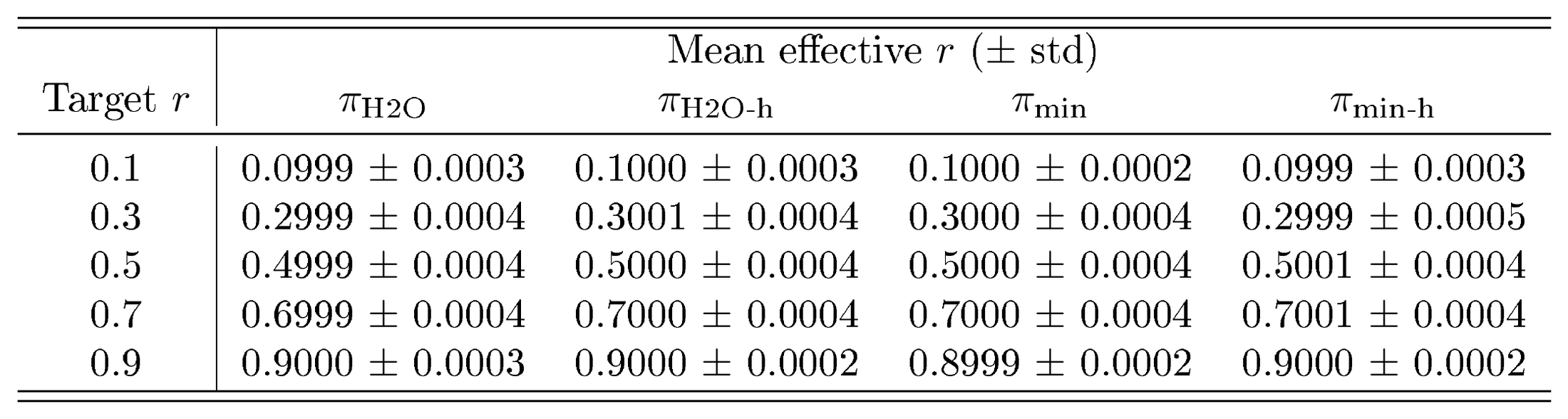
Table 1 empirically shows that when we set the target compression ratio in Algorithm 2, we obtain an effective compression ratio with minimal error.

::: {caption="Table 1: Difference between target and effective compression ratio is insignificant for Llama3 on the RULER dataset. Results are similar for Qwen3 and LongBench."}

:::

G. Experimental Details

We use the evaluation pipeline and implementations of SnapKV, TOVA, H2O, StreamingLLM, and K-norm available in KVPress v0.5.3 ([18]). All experiments are run on two NVIDIA RTX A6000 (48GB) and eight NVIDIA RTX A5000 (24GB). All experiments can be run on a 24GB GPU, taking approximately $3$ to $5$ seconds to completely run each example in either LongBench or RULER. The full research project required more compute than what is reported in the paper due to preliminary experiments as well as initial experimentation that either contained errors in implementation or were not as competitive.

$**Figure 7:** **Importance sampling temperature scaling pairwise win scores.** **Llama3** (top) and **Qwen3** (bottom) pairwise win scores at different importance sampling temperature scale values $\tau$.$

H. Minimum Variance Proposals and Priors

We define the following four proposal distributions

$ \begin{aligned} \pi_{\text{min}}(\mathbf{v}_i)\vcentcolon= \frac{p_t(\mathbf{v}_i)\cdot\lVert\mathbf{v}i\rVert}{\sum{j=1}^t p_t(\mathbf{v}j)\cdot\lVert\mathbf{v}j\rVert}, \qquad& \pi{\text{min-h}}(\mathbf{v}i)\vcentcolon=\frac{\sum{j=1}^t p_j(\mathbf{v}i)\cdot h_j\cdot\lVert\mathbf{v}i\rVert}{\sum{l=1}^t\sum{j=1}^t p_j(\mathbf{v}l)\cdot h_j\cdot\lVert\mathbf{v}l\rVert}, \ \pi{\text{H2O}}(\mathbf{v}i)\vcentcolon=\frac{\sum{j=1}^t p_j(\mathbf{v}i)}{\sum{l=1}^t \sum{j=1}^t p_j(\mathbf{v}l)}, \qquad & \pi{\text{H2O-h}}(\mathbf{v}i)\vcentcolon=\frac{\sum{j=1}^t p_j(\mathbf{v}i)\cdot h_j}{\sum{l=1}^t \sum{j=1}^t p_j(\mathbf{v}_l)\cdot h_j}; \end{aligned} $

where $h_j \vcentcolon=\left[(t-j+1)\cdot\mathcal{H}_t\right]^{-1}$ and $\mathcal{H}_t$ is the $t$-th harmonic number.

In this section, we discuss what exactly are the semantics of these distributions. Proposal $\pi_{\text{min}}$ is well known folklore result in the statistical methods literature ([9]). It is simply the proposal distribution that minimizes the variance for the expectation estimator for the last query attention value, i.e. $\mathbb{E}_{p_t}[\mathbf{V}]$: the expectation at eviction time. Notably, it is a proposal that uses the values of $\mathbf{V}$ in order to choose which entries to evict. None of the top- $k$ eviction methods we compare and study make use of both $p(\mathbf{V})$ and $\mathbf{V}$; see Appendix D for a description on how these eviction strategies compute their score.

Proposal $\pi_{\text{min-h}}$ extends this to all distributions ${p_i(\mathbf{V})}{i=1}^t$. To be precise, recall that the softmax matrix in Equation 5 $p(\mathbf{V})$ at eviction time $t$ (i.e. during the prefilling step) is $t\times t$. The first proposal $\pi{\text{min}}$ ignores all of the first $[1..t-1]$ rows, even though they may contain useful information to decide on which entries to evict. We interpret these rows as a random variable $T$ that, when used to condition the probability of eviction, tells you which entries are best to evict. That is,

$ \text{softmax}\left(\mathbf{Q}\cdot\mathbf{K}^{^{\mkern-1.5mu\mathsf{T}}}\right)=\left[p(\mathbf{V}|T=i)\right] _{i=1}^t.\tag{34} $

This assumes that there exists a distribution on $T$. We interpret this distribution $p(T)$ as some prior knowledge on how meaningful are each $p(\mathbf{V}|T=i)$ as $i$ distances from $t$. In both $\pi_{\text{min-h}}$ and $\pi$, we set this to

$ h_j \vcentcolon= p(T=j)=\frac{1}{(t-j+1)\cdot\mathcal{H}_t}.\tag{35} $

The semantics of this prior is simple: we assume that each row has exponentially diminishing importance: we weigh each row according to the following sequence $\mathbf{h}=\left[\frac{1}{t}, \frac{1}{t-1}, \dots, \frac{1}{3}, \frac{1}{2}, 1\right]$ and then normalize to get a probability distribution. The normalizing constant of sequence $\mathbf{h}$ is the harmonic number $\mathcal{H}t=\sum{k=1}^t\frac{1}{k}$, and the probability of each row is $p(T=i)=\left[(t-j+1)\cdot\mathcal{H}_h\right]^{-1}$

To then retrieve the probability of each entry $p(\mathbf{v}_i)$, we marginalize over all possible time steps

$ p(\mathbf{v}i)=\sum{j=1}^t p(\mathbf{v}i, T=j)=\sum{j=1}^t p(\mathbf{v}_i|T=j)\cdot p(T=j),\tag{36} $

which when using $p(T=j)=h_j$ for either the minimum variance proposal or the H2O proposal, yields $\pi_{\text{min-h}}$ and $\pi_{\text{H2O-h}}$ respectively. Note that any distribution for $p(T)$ is valid and results in a different proposal. In fact, any proposal that ignores the first $[1..t-1]$ rows contains a prior that is degenerated at $T=t$, with zero probability everywhere else.

I. Additional Experiments

In this section, we show additional experiments that supplement the claims in Section 7.

$**Figure 8:** **Importance sampling temperature scaling average total scores.** **Llama3** (top) and **Qwen3** (bottom) average total scores at different importance sampling temperature scale values $\tau$.$

I.1 Per Dataset Split Scores

We show the eviction scores for each of the four proposals defined in Section 7 and the five top- $k$ eviction methods—namely, Streaming LLM, SnapKV, TOVA, H2O and K-norm—across all of the splits of LongBench and some of RULER's. Due to space and time constraints, we only show six out of the 13 different splits in RULER.

Figure 5 shows the scores for Llama3 and Figure 6 shows the scores for Qwen3. In both cases, probabilistic eviction with correction tends to achieve better score performance. Notably, some eviction methods that do well in certain tasks. For example, on Llama3 StreamingLLM ranks first on the QuestionAnswer split, yet dead last in MultiKey-NIAH. Similarly, on Qwen3 K-norm is consistently in the top-3 on the MultiKey-NIAH split, yet last in CommonWords.

I.2 Importance Sampling Temperature

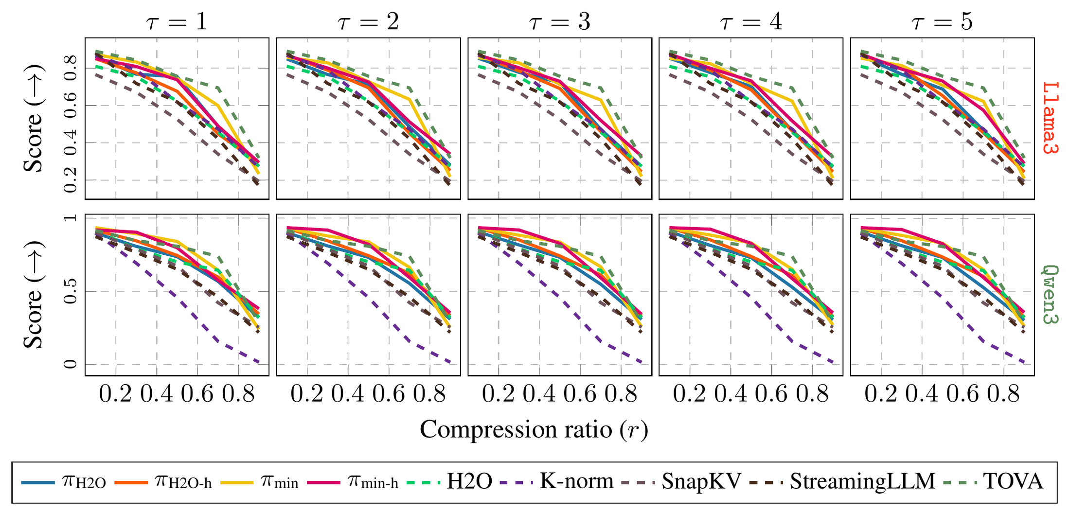
To further investigate the trade-off between bias and variance, we apply importance sampling temperature scaling to the same experimental setting as described in Section 7. Figure 8 and Figure 7 show the scores and pairwise win scores of RULER on Llama3 and Qwen3 across temperature values of $\tau\in{1, 2, 3, 4, 5}$. The plots show that, in most cases, the decrease in variance was not worth the increase in bias. This suggests that bias is the more important issue to resolve in KV eviction.

I.3 On the Behavior of Attention Head Compression Ratio

Given a fixed number of samples $m$, probabilistic eviction will automatically set the appropriate compression ratio of each head in accordance with that head's proposal distribution it samples from. This means that different attention heads might have very distinct compression ratios then others. Our findings show that this causes a distinct pattern in the distribution of attention head compression ratios. We find that lower (closer to the input) layers tend to be allocated more of the cache budget, while at higher (closer to the output) layers, less budget. This is a behavior that is reminiscent of [22]'s PyramidKV, where lower layers are given more of the KV cache budget.

Figure 9 shows this pattern for different proposal distributions. Notably, $\pi_{\text{min-h}}$ tends to act more conservatively, while $\pi_{\text{H2O}}$ spikes rapidly at certain layers.

J. Limitations

The ideal KV eviction method is not only zero-variance but also zero-bias. However, it is unrealistic to achieve this, as to do so, correction would have to be perfect, meaning that it can perfectly recreate the same KV cache from less memory than what was evicted. Our approach is also not perfect: self-normalized importance sampling is biased and has variance greater than zero. However, this estimator has reasonable upper bounds on bias and variance. This is in contrast to deterministic KV eviction methods that do not apply correction: these are zero-variance estimators but their bias is unbounded.

The bias of self-normalized importance sampling is upper bounded by $\mathcal{O} (m^{-1})$, where $m$ is the number of samples. This upper bound indicates that if there is less compression, then it will be more accurate—which is usually true for other eviction methods. Note that the inverse is not true: at a reasonable compression ratio, if the distributions at the attention heads are sparse, then the effective number of samples required to achieve a certain precision will be lower, meaning that in those cases even a higher compression ratio can achieve lower error.

In terms of implementation, we show that we are able to achieve distinct compression ratios at different heads. This requires a properly optimized KV eviction implementation to compute correction using an efficient sparse tensors implementation. This is addressed by [30], and can be extended to our case. Further, correction requires an additional memory overhead of $\mathcal{O} (k\cdot h\cdot b)$ bytes, where $k$ is the number of kept tokens, $h$ is the total number of attention heads in the LLM, and $b$ is the floating point precision in bytes. Asymptotically, this is dwarfed by the KV cache size itself and not a real concern, as the cache size is $\mathcal{O} (d\cdot k\cdot h\cdot b)$, where $d$ is the embedding dimension.

References

Section Summary: This section compiles a list of academic papers and technical reports primarily on optimizing large language models for longer contexts. It emphasizes methods for compressing and quantizing the key-value cache, refining attention mechanisms, and applying statistical sampling techniques to reduce memory demands during inference. Additional entries cover model architectures, benchmarks for long-context evaluation, and foundational work on transformers and Monte Carlo methods.

[1] Hooper et al. (2024). KVQuant: Towards 10 Million Context Length LLM Inference with KV Cache Quantization. In Advances in Neural Information Processing Systems. pp. 1270–1303. doi:10.52202/079017-0040. https://proceedings.neurips.cc/paper_files/paper/2024/file/028fcbcf85435d39a40c4d61b42c99a4-Paper-Conference.pdf.

[2] Amir Zandieh et al. (2026). TurboQuant: Online Vector Quantization with Near-optimal Distortion Rate. In The Fourteenth International Conference on Learning Representations. https://openreview.net/forum?id=tO3ASKZlok.

[3] Adam Zweiger et al. (2026). Fast KV Compaction via Attention Matching. https://arxiv.org/abs/2602.16284. arXiv:2602.16284.

[4] Sabri Eyuboglu et al. (2025). Cartridges: Lightweight and general-purpose long context representations via self-study. https://arxiv.org/abs/2506.06266. arXiv:2506.06266.

[5] Xiao et al. (2024). Efficient Streaming Language Models with Attention Sinks. In International Conference on Learning Representations. pp. 21875–21895. https://proceedings.iclr.cc/paper_files/paper/2024/file/5e5fd18f863cbe6d8ae392a93fd271c9-Paper-Conference.pdf.

[6] Li et al. (2024). SnapKV: LLM Knows What You are Looking for Before Generation. In Advances in Neural Information Processing Systems. pp. 22947–22970. doi:10.52202/079017-0722. https://proceedings.neurips.cc/paper_files/paper/2024/file/28ab418242603e0f7323e54185d19bde-Paper-Conference.pdf.

[7] Oren et al. (2024). Transformers are Multi-State RNNs. In Proceedings of the 2024 Conference on Empirical Methods in Natural Language Processing. pp. 18724–18741. doi:10.18653/v1/2024.emnlp-main.1043. https://aclanthology.org/2024.emnlp-main.1043/.

[8] Zhang et al. (2023). H2O: Heavy-Hitter Oracle for Efficient Generative Inference of Large Language Models. In Advances in Neural Information Processing Systems. pp. 34661–34710. https://proceedings.neurips.cc/paper_files/paper/2023/file/6ceefa7b15572587b78ecfcebb2827f8-Paper-Conference.pdf.

[9] Art B. Owen (2013). Monte Carlo theory, methods and examples. https://artowen.su.domains/mc/.

[10] S. Agapiou et al. (2017). Importance Sampling: Intrinsic Dimension and Computational Cost. Statistical Science. 32(3). pp. 405 – 431. doi:10.1214/17-STS611. https://doi.org/10.1214/17-STS611.

[11] Vaswani et al. (2017). Attention is All you Need. In Advances in Neural Information Processing Systems. pp. . https://proceedings.neurips.cc/paper_files/paper/2017/file/3f5ee243547dee91fbd053c1c4a845aa-Paper.pdf.

[12] Devoto et al. (2024). A Simple and Effective $L_2$ Norm-Based Strategy for KV Cache Compression. In Proceedings of the 2024 Conference on Empirical Methods in Natural Language Processing. pp. 18476–18499. doi:10.18653/v1/2024.emnlp-main.1027. https://aclanthology.org/2024.emnlp-main.1027/.

[13] T. Kloek and H. K. van Dijk (1978). Bayesian Estimates of Equation System Parameters: An Application of Integration by Monte Carlo. Econometrica. 46(1). pp. 1–19. http://www.jstor.org/stable/1913641.

[14] John Geweke (1989). Bayesian Inference in Econometric Models Using Monte Carlo Integration. Econometrica. 57(6). pp. 1317–1339. http://www.jstor.org/stable/1913710.

[15] Cardoso et al. (2022). BR-SNIS: Bias Reduced Self-Normalized Importance Sampling. In Advances in Neural Information Processing Systems. pp. 716–729. https://proceedings.neurips.cc/paper_files/paper/2022/file/04bd683d5428d91c5fbb5a7d2c27064d-Paper-Conference.pdf.

[16] Ainslie et al. (2023). GQA: Training Generalized Multi-Query Transformer Models from Multi-Head Checkpoints. In Proceedings of the 2023 Conference on Empirical Methods in Natural Language Processing. pp. 4895–4901. doi:10.18653/v1/2023.emnlp-main.298. https://aclanthology.org/2023.emnlp-main.298/.

[17] Aaron Grattafiori et al. (2024). The Llama 3 Herd of Models. https://arxiv.org/abs/2407.21783. arXiv:2407.21783.

[18] Devoto et al. (2025). Expected Attention: KV Cache Compression by Estimating Attention from Future Queries Distribution. arXiv preprint arXiv:2510.00636. https://arxiv.org/abs/2510.00636.

[19] An Yang et al. (2025). Qwen3 Technical Report. https://arxiv.org/abs/2505.09388. arXiv:2505.09388.

[20] Yushi Bai et al. (2024). LongBench: A Bilingual, Multitask Benchmark for Long Context Understanding. https://arxiv.org/abs/2308.14508. arXiv:2308.14508.

[21] Cheng-Ping Hsieh et al. (2024). RULER: What's the Real Context Size of Your Long-Context Language Models?. https://arxiv.org/abs/2404.06654. arXiv:2404.06654.

[22] Zefan Cai et al. (2025). PyramidKV: Dynamic KV Cache Compression based on Pyramidal Information Funneling. In Second Conference on Language Modeling. https://openreview.net/forum?id=ayi7qezU87.

[23] Chen et al. (2025). The Pitfalls of KV Cache Compression. arXiv preprint arXiv:2510.00231.

[24] Ryan Singh and Christopher L. Buckley (2023). Attention: Marginal Probability is All You Need?. https://arxiv.org/abs/2304.04556. arXiv:2304.04556.

[25] Arthur S. Bianchessi et al. (2026). Bayesian Attention Mechanism: A Probabilistic Framework for Positional Encoding and Context Length Extrapolation. In The Fourteenth International Conference on Learning Representations. https://openreview.net/forum?id=dXJB9O8fLd.

[26] Brent, Richard P. and Zimmermann, Paul (2010). Modern Computer Arithmetic. Cambridge University Press.

[27] Erdős, Paul and Rényi, Alfréd (1961). On a classical problem of probability theory. Magyar Tudományos Akadémia Matematikai Kutató Intézetének Kőzleményei. https://www.renyi.hu/~$p_e$rdos/1961-09.pdf.

[28] Philippe Flajolet et al. (1992). Birthday paradox, coupon collectors, caching algorithms and self-organizing search. Discrete Applied Mathematics. 39(3). pp. 207-229. doi:https://doi.org/10.1016/0166-218X(92)90177-C. https://www.sciencedirect.com/science/article/pii/0166218X9290177C.

[29] Robert Z (https://math.stackexchange.com/users/299698/robert-z). Expected number of non-empty boxes. Mathematics Stack Exchange. URL:https://math.stackexchange.com/q/1950447 (version: 2016-10-02). https://math.stackexchange.com/q/1950447.

[30] Yuan Feng et al. (2026). Ada-KV: Optimizing KV Cache Eviction by Adaptive Budget Allocation for Efficient LLM Inference. In The Thirty-ninth Annual Conference on Neural Information Processing Systems. https://openreview.net/forum?id=tcisuhGsQZ.