Storing Infinite Dynamical Attractors in Nonreciprocal Associative Neural Networks

Miguel Aguilera
BCAM -- Basque Center for Applied Mathematics, 48009 Bilbao, Spain

Daniele De Martino
Biofisika Institute (CSIC, EHU), 48940 Leioa, Spain

Abstract

We develop a dynamical mean-field theory for nonreciprocal associative networks that store an extensive number of dynamical attractors, from limit cycles to strange attractors. Using a path integral calculation under quenched disorder, we derive self-consistent dynamical mean-field equations for pattern overlaps, autocorrelations and response functions. Memory retrieval capacity is governed by the spectral structure of the coupling matrices encoding stored patterns. When their eigenvalues are coherently aligned, retarded self-interactions and quenched noise feed back destructively: at zero eigenphase (fixed point attractors) the classical equilibrium capacity bound is recovered, while for limit cycles retrieval collapses far below it. In contrast, for uniformly distributed eigenphases, retarded self-interactions and much of the quenched noise cancels, reducing the dynamics to an effective single-spin process and amplifying capacity substantially. We validate the theory against microscopic simulations for limit-cycle and chaotic attractors, identifying eigenvalue decoherence as the mechanism enabling enhanced storage of dynamical memories.

Biological neural circuits sustain multiple oscillatory rhythms simultaneously, spanning distinct timescales and coexisting within the same circuits [1, 2].

Such multiplicity is a long-standing theme in systems neuroscience [3, 4], proposed to support a code in which different frequency bands carry distinct information streams [5].

Statistical mechanics has proven fundamental to understanding how neural network models function as associative memories [6, 7], but it remains an open question how a recurrent network can simultaneously store an extensive number of distinct dynamical attractors, each with its own temporal structure.

Analytical studies of associative memory have largely focused on the storage of static patterns [8, 9], with symmetric interactions among neuronal units.

Nonreciprocal (asymmetric) couplings extend this to sequential association [10, 11, 12, 13, 14] and oscillations [15, 16], but the capacity of such networks has been characterized only for a single stored sequence or cycle [17, 18] and nonreciprocal diluted systems retrieving static patterns [19, 20, 21].

Similar nonreciprocal Hebbian structures underlie linear attention mechanisms [22]. Exponential hetero-associative networks have become an active object of study to characterise nonlinear attention [23, 24], connecting the memory capacity of sequential memories to modern transformer architectures.

Here we develop a a dynamical mean-field theory for nonrecirocal associative memories that encode an extensive number of dynamical attractors with distinct frequencies and structure, and we show that the retrieval capacity is governed by the spectral structure of the couplings between encoded patterns.

Model— We consider a network of $N$ binary spins, $\bm x_t=(x_{1,t},\ldots,x_{N,t})$, with $x_{i,t}\in{\pm1}$ and $t=0,\ldots,\mathcal T$. Spins are updated stochastically in discrete time, with update probability $\Delta$, driven by effective fields $\bm h_t=(h_{1,t},\ldots,h_{N,t})$ defined as

Executive Summary: Nonreciprocal associative networks can in principle store many dynamical patterns such as limit cycles and chaotic orbits, yet the conditions that allow extensive storage have remained unclear. The central problem is to determine how recurrent networks with asymmetric couplings sustain multiple independent temporal attractors without destructive interference, a question motivated by the coexistence of distinct oscillatory rhythms observed in cortical circuits.

The work develops a dynamical mean-field theory that tracks pattern overlaps, response functions and noise correlations for networks storing an extensive number of such attractors. It derives closed equations for the order parameters by averaging a path-integral representation over quenched random patterns and validates the resulting predictions against large-scale microscopic simulations.

The analysis shows that retrieval capacity is controlled by the distribution of eigenvalues of the matrices that encode the stored patterns. When all eigenvalues share the same phase, retarded self-interactions reinforce quenched noise and capacity collapses well below the classical Hopfield limit once genuine oscillations appear. When eigenvalues are spread uniformly around the unit circle, these cross terms largely cancel, the effective dynamics reduces to a simpler single-spin process, and capacity roughly doubles. The same amplification occurs for a chaotic attractor when its two conjugate eigenvalue pairs are drawn from a broad phase distribution. Direct simulations confirm that gradually increasing phase diversity across attractors raises capacity by a factor of 1.5 to 3 for most frequencies.

These results indicate that spectral diversity, rather than the specific topology of the attractors, is the decisive factor that permits many dynamical memories to coexist. The finding reverses the usual expectation that greater complexity reduces stability and supplies a functional rationale for the incommensurate frequency bands observed in hippocampus and cortex.

The theory requires that the spectral radius of the response matrix remain below one and that the patterns remain random; it has been tested only for intermediate update rates and for attractors whose encoding matrices are orthogonal. Further work is needed to relax these restrictions and to test whether biological circuits exploit eigenvalue diversity to maintain multiple rhythms.

$ h_{i,t}=H_{i,t}+\sum_{j; j\neq i} J_{ij}x_{j,t}, $

where $H_{i,t}$ are time-dependent external fields.

Couplings $J_{ij}$, with $J_{ii}=0$, are constructed from $1+L$ blocks of interacting random patterns.

Each block $\upsilon$ encodes one dynamical attractor, each containing $M_\upsilon$ patterns $\bm\xi_\upsilon^a=(\xi_{1,\upsilon}^a,\ldots,\xi_{N,\upsilon}^a)$. Patterns are composed by i.i.d. random variables $\xi_{i,\upsilon}^a\in{\pm1}$, coupled through an $M_\upsilon\times M_\upsilon$ matrix $\bm A^\upsilon$:

$ J_{ij} =\frac{1}{N}\sum_{\upsilon=0}^{L} \sum_{a,b=1}^{M_\upsilon} A_{ab}^\upsilon\xi_{i,\upsilon}^a\xi_{j,\upsilon}^b, \qquad i\neq j. $

Trajectories $\bm x={\bm x_0,\dots,\bm x_{\mathcal T}}$ evolve through stochastic updates governed by independent variables $\tau_{i,t}\sim\mathrm{Bernoulli}(\Delta)$, which determine whether spin $i$ is updated at time $t$ via Glauber dynamics at inverse temperature $\beta=1/T$ ($\tau_{i,t}=1$), or held fixed ($\tau_{i,t}=0$). For a given field history $\bm h={\bm h_0,\dots,\bm h_{\mathcal T}}$, this defines the path probability

$ \begin{aligned} p_{\bm h}(\bm x, \bm \tau) =& \prod_{i,t} p(\tau_{i,t+1}) \big( (1-\tau_{i,t+1}) \delta_{x_{i,t+1},x_{i,t}} \nonumber\ & + \tau_{i,t+1} \frac{1}{2} (1+ x_{i,t} \tanh[\beta h_{i,t}]) \big). \end{aligned} $

The parameter $\Delta$ interpolates between parallel dynamics ($\Delta=1$) and single–spin updates ($\Delta\to 0$); for all numerical results in this Letter we use an intermediate value $\Delta=0.1$.

Note that leaving $\bm h$ as a generic function allows us to later introduce the self-consistent fields from our mean-field theory.

Quenched disorder and order parameters— We single out block patterns for $\upsilon=0$ as the target sequential memory, and split the patterns into this main target set and the remaining $P:=\sum_{\upsilon=1}^{L}M_\upsilon$ sets as a source of quenched disorder,

$ \begin{aligned} J_{ij} &= \frac{1}{N} \bm\xi_i^\top \bm A \bm\xi_j + \frac{1}{N} \bm{\hat{\xi}}_i^\top \bm{\hat{A}} \bm{\hat{\xi}}_j, \qquad i \neq j, \end{aligned} $

with the target pattern $\bm \xi_i \coloneqq \bm \xi_{i,0}$, $\bm A \coloneqq \bm A^0$ (with $M=M_0$), and joint patterns $\bm{\hat{\xi}}i \coloneqq (\bm \xi{i,1},\dots, \bm \xi_{i,P})$ and couplings $\bm{\hat{A}} \coloneqq \mathrm{diag}(\bm A^1, \ldots, \bm A^L)$. The memory load per spin is defined as $\alpha = P/N$.

Dynamical mean-field theory— We introduce a moment-generating functional for trajectories, for each realization of $\bm{\hat{\xi}}$, adding fields $\bm g$:

$ \begin{aligned} Z_{\bm{\hat{\xi}}}(\bm g) &= \left\langle e^{\sum_{i,t} x_{i,t} g_{i,t}} \right\rangle_{\bm h}, \end{aligned} $

with $\langle f(\bm x)\rangle_{\bm h} = \sum_{\bm x, \bm \tau} p_{\bm h}(\bm x, \bm \tau) f(\bm x)$.

Derivatives of $Z_{\bm{\hat{\xi}}}(\bm g)$ retrieve spin moments, e.g., $\partial Z_{\bm{\hat{\xi}}}(\bm 0)/\partial g_{i,t} = \left\langle x_{i,t}\right\rangle_{\bm h}$, and response functions, ${\partial^2 Z_{\bm{\hat{\xi}}}(\bm 0)}/(\partial g_{i,t}\partial H_{j,s}) = {\partial \left\langle x_{i,t}\right\rangle_{\bm h}}/{\partial H_{j,s}}$.

We define dynamical order parameters for the pattern overlaps, correlations, and response functions:

$ \begin{aligned} m_t^a &= \frac{1}{N}\sum_i \xi_i^a \frac{\partial Z_{\bm{\hat{\xi}}}(\bm 0)}{\partial g_{i,t}} = \frac{1}{N}\sum_i \xi_i^a \left\langle x_{i,t}\right\rangle_{\bm h}, \quad\text{(a)}\ q_{t,s} &= \frac{1}{N}\sum_i \frac{\partial^2 Z_{\bm{\hat{\xi}}}(\bm 0)}{\partial g_{i,t}\partial g_{i,s}} = \frac{1}{N}\sum_i \left\langle x_{i,t}x_{i,s}\right\rangle_{\bm h}, \quad\text{(b)}\ \chi_{t,s} &= \frac{1}{N}\sum_i \frac{\partial^2 Z_{\bm{\hat{\xi}}}(\bm 0)}{\partial g_{i,t}\partial H_{i,s}} \nonumber\ &= \frac{\beta}{N}\sum_i \left\langle x_{i,t} \tau_{i,s+1}(x_{i,s+1} - \tanh[\beta h_{i,s}])\right\rangle_{\bm h}, \quad\text{(c)} \end{aligned} $

We also introduce $\rho_{t,s}= N^{-1} \sum_i{\partial^2 Z_{\bm{\hat{\xi}}}(\bm 0)}/(\partial H_{i,t}\partial H_{i,s})$, which becomes equal to zero as $\partial Z_{\bm{\hat{\xi}}}(\bm 0)/\partial H_{i,t}=0$.

To obtain closed equations for the order parameters, we follow a path-integral approach [25, 7] to calculate the average $\langle\langle{Z_{\bm{\hat{\xi}}}(\bm g)}\rangle\rangle = \sum_{\bm{\hat{\xi}}} p(\bm{\hat{\xi}}) Z_{\bm{\hat{\xi}}}(\bm g)$ over uniformly distributed independent patterns $\xi_{i,\upsilon}^a$ for $\upsilon>0$ so $p(\bm{\hat{\xi}}) = 2^{-P}$. We introduce the order parameters above plus additional auxiliary variables via integral representations of delta functions to allow averaging over quenched disorder (see SM [26] for a detailed calculation, a summary of which is reported in End matter). Finally saddle-point evaluation results in the quenched generating functional

$ \begin{aligned} \langle\langle{Z_{\bm{\hat{\xi}}}(\bm g)}\rangle\rangle \propto & \int d\bm z p(\bm z) \frac{1}{2^M}\sum_{\bm\sigma} \left\langle e^{\sum_{i,t}x_{i,t} g_{i,t}}\right\rangle_{\bm {\tilde{h}}^{\bm\sigma}}. \ {\tilde{h}}{i,t}^{\bm\sigma} &= H{i,t} + \sum_{ab}\sigma_a A_{ab} m_t^b + \alpha\sum_{s; s<t} K_{t,s} x_{i,s} + z_{i,t}. \end{aligned} $

Here, we represent the realizations of $\bm{\xi}_i = (\xi_i^1,\ldots,\xi_i^M)$ by a binary vector $\bm{\sigma}\in{\pm1}^M$ with $2^M$ possible states (with $M=M_0$).

The term $\bm z_i = (z_{i,0}, \dots, z_{i,\mathcal T})$ is a Gaussian variable determined by $p(\bm z_i) \sim \mathcal{N}(\bm 0, \alpha\bm R)$.

The result relies on the kernels $\bm R, \bm K$, defined as functions of $\bm q, \bm \chi$ and $\bm{\hat{A}}$

$ \begin{aligned} R_{t,s} &= \frac{1}{P} \sum_{a=0}^{P-1} \big[\bm\kappa^{-1} \big(\bm I_P \otimes \bm q\big) \bm\kappa^{-\top} \Big]{(aT+t,aT+s)}, \quad\text{(a)} \ K{t,s} &= \frac{1}{P} \sum_{a=0}^{P-1} \big[-\bm\kappa^{-1} \big]{(aT+t,aT+s)}, \ \bm\kappa & \coloneqq \bm I_P\otimes\bm\chi - \bm{\hat{A}}^{-1}\otimes\bm I{\mathcal T}. \quad\text{(b)} \end{aligned} $

being $\otimes$ the Kroneker product and where $\bm\kappa^{-\top} = (\bm\kappa^{\top})^{-1}$.

Note that the diagonal exclusion $J_{ii}=0$ generates an Onsager correction that cancels $K_{t,t}$ exactly (see End Matter), so the retarded kernel couples $x_{t+1}$ only to spins at $s<t$.

The result above can be simplified in the case of an orthonormal matrix $\bm{\hat{A}}$ with eigenvalues ${\hat\lambda_r}$ yielding

$ \begin{aligned} \bm R &= \frac{1}{P} \sum_{n,m=0}^\infty \sum_{r=1}^{P} \hat\lambda_r^{n+1}(\hat\lambda_r^\ast)^{m+1} \bm\chi^n \bm q (\bm\chi^\top)^m, \quad\text{(a)} \ \bm K &=\frac{1}{P} \sum_{n=0}^\infty \sum_{r=1}^P \hat\lambda_r^{n+1} \bm\chi^n. \quad\text{(b)} \end{aligned} $

As $\bm\chi$ is strictly lower diagonal, Eqs. (8a-Equation 8b) can be computed at time $t+1$ using only causal influences from time $s\le t$ (see Equation 16a-Equation 16b in the End Matter).

Furthermore, the equation above results in diverging $\bm R, \bm K$ when the spectral radius of $\bm\chi$ is larger than 1. This predicts that memory retrieval will be unfeasible beyond that point (quenched noise is amplified indefinitely).

Mean-field equations— The quenched generating functional Equation 6 factorises over spins once the kernels $\bm R$ and $\bm K$ are fixed.

Dropping $i$ terms for simplicity, for zero fields and orthonormal $\bm{\hat{A}}$, we describe the behaviour of the system with simplified mean-field equations

$ \begin{aligned} \bm m_{t} &= \frac{1}{2^M}\sum_{\bm\sigma} \bm\sigma \left\langle x_{t}\right\rangle_{\bm {\tilde{h}}^{\bm\sigma}} \quad\text{(a)} \ \chi_{t,s} &= \frac{\beta}{2^M}\sum_{\bm\sigma} \left\langle x_{t} \tau_{s+1}(x_{s+1} - \tanh[\beta {\tilde{h}}s])\right\rangle{\bm {\tilde{h}}^{\bm\sigma}}, \quad\text{(b)} \end{aligned} $

Two-time correlations propagate recursively. For $t>s$,

$ \begin{aligned} q_{t+1,s} &=(1-\Delta)q_{t,s} +\left\langle \tau_{t+1}x_{t+1}x_s\right\rangle_ {\bm{\bar{h}}^{\bm\sigma}}, \ \left\langle \tau_{t+1}x_{t+1}x_{s+1}\right\rangle_ {\bm{\bar{h}}^{\bm\sigma}} &=(1-\Delta) \left\langle \tau_{t+1}x_{t+1}x_s\right\rangle_ {\bm{\bar{h}}^{\bm\sigma}} \nonumber\ &\quad+ \left\langle \tau_{t+1}\tau_{s+1} x_{t+1}x_{s+1}\right\rangle_ {\bm{\bar{h}}^{\bm\sigma}} . \end{aligned} $

and, for $t\neq s$,

$ \left\langle \tau_{t+1}\tau_{s+1}x_{t+1}x_{s+1}\right\rangle_ {\bm{\bar{h}}^{\bm\sigma}} = \frac{\Delta^2}{2^M} \sum_{\bm\sigma} \left\langle \tanh(\beta\bar{h}_t^{\bm\sigma}) \tanh(\beta\bar{h}s^{\bm\sigma}) \right\rangle{\bm{\bar{h}}^{\bm\sigma}}. $

Solving these equations is made intractable by the self-dependence of $\bm x$ through couplings $\bm K$ and the non-Markovian history encoded in $\bm R$. The mean field behaviour can be estimated by Monte Carlo sampling of the effective single-spin process (similarly to [27]), or directly solving the equations in special cases where $\bm K=\bm 0$.

Encoding identical cycles— Since matrices $\bm A^\upsilon$ are real, their eigenvalues come in conjugate pairs $e^{\pm \mathrm{i}\mkern1mu\phi_r}$ (with an additional $\pm1$ eigenvalue when the dimension is odd).

We first consider the simplest case of identical $2{\times}2$ rotation matrices $\bm A^\upsilon=\bm A = \bm \Omega_\phi$, where $\bm \Omega_\phi \coloneqq \left[\begin{smallmatrix} \cos\phi & \sin\phi\ -\sin\phi & \cos\phi\end{smallmatrix}\right]$.

This yields

$ \begin{aligned} \bm R &= \sum_{n,m=0}^\infty \cos((n-m)\phi) \bm\chi^n \bm q (\bm\chi^\top)^m, \ \bm K &= \sum_{n=0}^\infty \cos((n+1)\phi)\bm\chi^n. \end{aligned} $

Decomposing $\bm R = \operatorname{Re}[\bm S]$ and $\bm K = \operatorname{Re}[\bm G]$ with complex auxiliary matrices, the order parameters satisfy $\bm S = \bm q + e^{\mathrm{i}\mkern1mu\phi}\bm\chi\bm S + e^{-\mathrm{i}\mkern1mu\phi}\bm S\bm\chi^\top - \bm\chi\bm S\bm\chi^\top, \bm G = e^{\mathrm{i}\mkern1mu\phi}!\left(\bm I + \bm\chi\bm G\right)$ which can be solved forward in time exploiting the strictly lower-triangular (causal) structure of $\bm\chi$.

The rotation angle $\phi$ interpolates between qualitatively different dynamical regimes.

For $\phi=0$ the attractors are fixed points, recovering the results of a classical Hopfield network (similar to [9]) but for partially parallel dynamics.

As $\phi$ increases from zero the network can sustain genuine cyclic orbits, and the critical capacity drops sharply.

Already at zero load the dynamics undergoes a heteroclinic bifurcation at $\beta^*(\phi)$, where the cycle slows near four saddle-type fixed points until its period diverges and the orbit collapses onto fixed points (see End Matter; see also Ref. [28]).

This boundary also appears in Figure 1(a): warm-colored curves lie on the fixed-point side of $\beta^*$ and decay slowly, cooler ones retrieve limit cycles.

Once oscillations emerge, the retarded self-interaction $\bm K$ and the cross-terms in $\bm R$ feed back destructively, drastically reducing the number of storable patterns.

Encoding cycles with isotropic eigenvalues— A remarkable simplification occurs when the eigenvalues of $\bm{\hat{A}}$ are uniformly distributed on the unit circle.

The sums over eigenvalues in Equation 8b and over conjugate pairs in Equation 8a are equal to zero except the latter when $n=m$, resulting in

$ \bm R = \sum_{n=0}^\infty \bm\chi^n \bm q (\bm\chi^\top)^n, \qquad \bm K = 0. $

The new form allows us to write $\bm R$ in the form of the Lyapunov equation $\bm R=\bm q+\bm\chi \bm R \bm\chi^\top$, and the absence of $\bm K$ eliminates the delayed self-coupling rendering the effective single-spin dynamics equivalent to a nonequilibrium spin glass driven by coloured Gaussian noise.

For uniform eigenvalues on the unit circle, the stochastic update of the mean-field equations reads

$ \bm m_{t+1}=(1-\Delta)\bm m_t +\frac{\Delta}{2^M}\sum_{\bm\sigma} \bm\sigma\int Dz_t \tanh[\beta {\tilde{h}}_t^{\bm\sigma}], $

with susceptibility, for $t>s$,

$ \chi_{t,s}=\Delta (1-\Delta)^{t-s-1} \frac{\beta}{2^M}\sum_{\bm\sigma}\int Dz_s \Big(1-\tanh^2[\beta {\tilde{h}}_s^{\bm\sigma}]\Big), $

where $Dz=dz\frac{1}{\sqrt{2\pi}}e^{-\frac{1}{2}z^2}$.

In this case, we can solve the self-consistent equations directly without recurring to Monte Carlo methods. Figure 1(b) shows the resulting phase boundary $\alpha_c$ for independent rotation matrices $\bm A^\upsilon = \bm \Omega_{\phi_\upsilon}$ with angles $\phi_\upsilon$ sampled uniformly from $[0,2\pi)$, so that each stored attractor oscillates at a different, randomly chosen frequency.

The $\phi=0$ curve shows $\alpha_c(T=0)\simeq 0.27$, roughly twice the classical Hopfield capacity of $0.138$. This parallels the result in [17] for a single infinite-length sequence at $\Delta = 1$, whose solution is equivalent to the equilibrium solution of the system at $\phi=0$ for any $\Delta$. All other curves interpolate smoothly toward it, suggesting the destructive feedback responsible for the capacity collapse in Figure 1(a) is an artifact of coherent eigenphase alignment rather than an intrinsic cost of storing cyclic attractors.

Compared with the single-angle case (Figure 1(a)), the memory capacity is greatly amplified: for all angles the capacity substantially exceeds that of the corresponding limit-cycle regime. The exception is the edge case $\phi=0.3\pi$. We find attractors beyond $\phi\approx 0.32\pi$ cannot be stored at all, and memory retrieval fails even for infinitely small $\alpha$. This is predicted nicely by our theory. For $\alpha=0$, we find for large $\beta$ a transition (see Figure 4) where the spectral value of $\bm\chi$ becomes larger than 1, making $\bm R$ diverge for large t. Thus, near this limit the memory capacity is reduced instead of amplified.

Retrieval of a chaotic attractor— The framework extends naturally to higher-dimensional coupling matrices.

For $M = 4$, a real orthogonal matrix $\bm A$ has two conjugate eigenvalue pairs $e^{\pm \mathrm{i}\mkern1mu\phi_1}$, $e^{\pm \mathrm{i}\mkern1mu\phi_2}$.

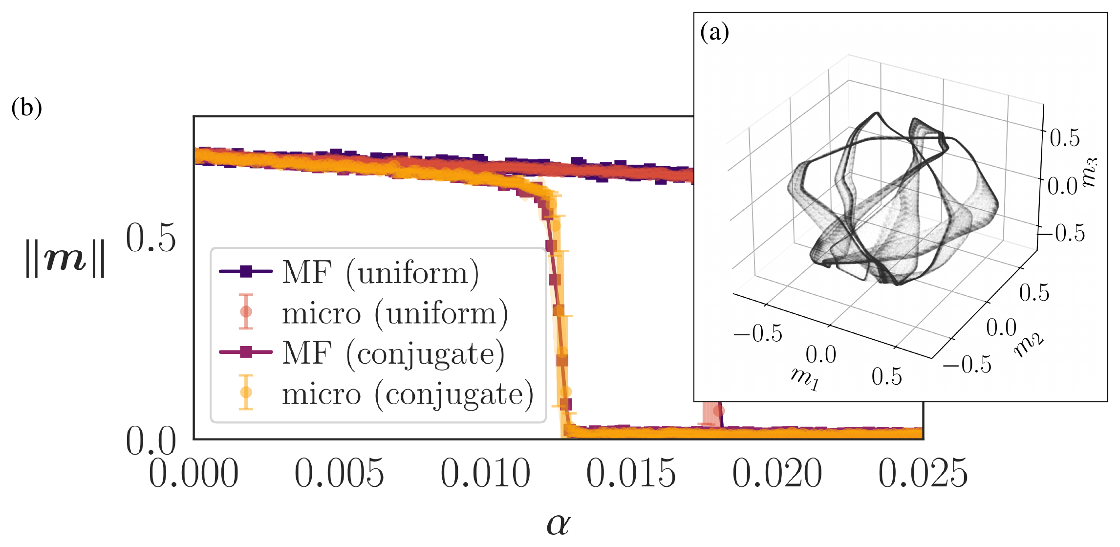
For suitable choices of $\bm A$ this orbit can become quasiperiodic or chaotic. We used a genetic algorithm (see SM) to find matrices $\bm A$ resulting in chaotic dynamics for $\alpha=0$ and spectral radius of $\bm\chi$ smaller than one to ensure the attractor can be stored in memory. Figure 2(a) shows a strange attractor obtained by this procedure, with $\phi_1\approx 0.23\pi$, $\phi_2\approx 1.73\pi$, and Lyapunov exponents $\lambda_1\approx 0.032$, $\lambda_2\approx -0.001$, projected onto the first three pattern overlaps.

Figure 2(b) shows the memory capacity of this chaotic attractor for the conjugate and uniform eigenvalue distributions, respectively (see End matter).

In both cases the mean-field prediction agrees quantitatively with microscopic simulations, validating the mean-field description of chaotic attractor retrieval under quenched disorder.

As in the limit-cycle regime, the uniform distribution yields a higher critical load than the conjugate one, supporting the hypothesis that eigenvalue decoherence amplifies memory capacity independently of the attractor topology.

{width=80%}

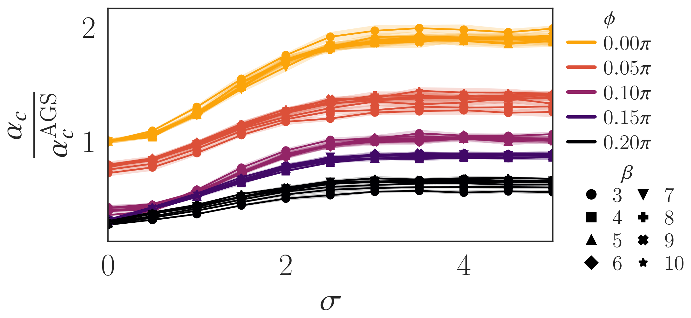
Partial coherence— The results above suggest that it is the diversity of eigenphases across stored attractors that controls the memory capacity. To test this directly, we come back to the case of storing 2D limit cycles, this time by drawing each eigenphase from a normal distribution centred at a common angle $\phi$ with standard deviation $\sigma$, so that $\sigma=0$ recovers the fully coherent case of Figure 1(a) and increasing $\sigma$ progressively decorrelates the phases across attractors, . through numerical simulations with $N=50,000$ spins. Figure 3 shows the resulting critical capacity $\alpha_c(\beta,\sigma,\phi)$ for several central angles $\phi$ and inverse temperatures $3\leq\beta\leq 10$, normalized by the classical memory capacity solution $\alpha^\mathrm{AGS}(\beta) = \alpha_c(\beta,0,0)$ at $\phi=0$ [9] and a factor $f(\phi)$ minimising the mean squared error between $\alpha_c(\beta,0,\phi)$ and $\alpha^\mathrm{AGS}(\beta)f(\phi)$. For all but the largest $\phi$, capacity increases monotonically with $\sigma$, improving memory capacity by a factor between 1.5 and 3. Note that large values of $\phi$, too close to the instability boundary, do not display a memory enhancement with phase decoherence.

{width=70%}

Discussion— Recurrent networks with nonreciprocal Hebbian couplings can store an extensive number of dynamical attractors, provided the response matrix $\bm\chi$ has a spectral radius smaller than one. The resulting memory capacity crucially depends on the spectral structure of the encoding matrices $\bm{\hat{A}}$.

Since coherent eigenphases make the cross-terms in $\bm R$ and the retarded couplings $\bm K$ feed back destructively while decoherence cancels both, it is the spectral diversity of the stored attractors, rather than their dynamical topology, that sets how many of them can coexist.

Both quantities also simplify by other mechanisms. In diluted networks [19, 7], $\bm R$ collapses onto the spin autocorrelation, while $\bm K$ is also eliminated for fully asymmetric dilutions. As in the case of eigenvalue decoherence, dilution severs crosstalk interactions among patterns.

From a biological perspective, the coexistence of multiple oscillatory modes with incommensurate frequencies is ubiquitous in hippocampal and cortical circuits [29, 2], with different bands carrying different information streams [30].

Our results give this spectral diversity a functional rationale: attractors spanning incommensurate frequencies interfere less, so capacity grows with the spread of eigenphases.

In the more general context of complex systems dynamics the fact that diversity amplifies rather than degrades capacity runs against the intuition, formalised by May [31, 32], that complexity destabilises large interacting systems.

Analogous inversions appear elsewhere: from heterogeneous excitability tuning stability in excitatory-inhibitory neural networks [33] to diversity of species in generalized Lotka-Volterra models with sublinear population growth promoting stability [34].

In each case, a form of diversity (eigenphases, excitability thresholds, or number of species) turns increasing complexity from a source of instability into a stabilising force.

Acknowledgements

Section Summary: The acknowledgements section outlines the various sources of financial and institutional support for the researchers M.A. and D.D.M. M.A. receives backing through Spain's Ramón y Cajal program, multiple national grants from the Ministry of Science and related agencies, European Union funds, and several Basque Government initiatives, including programs at the BCAM research center. D.D.M. is supported by additional grants from the Basque Government and a project funded jointly by Spanish agencies and European regional development funds.

Acknowledgments

M.A. is partly supported by the Ramón y Cajal programme (RYC2022-038204-I), funded by MICIU/AEI/10.13039/501100011033 and by the European Social Fund Plus (FSE+), Grant PID2023-146869NA-I00 funded by MICIU/AEI/10.13039/501100011033 and cofunded by the European Union, and Basque Government ELKARTEK funding (code KK-2023/00085). He is also supported by the Basque Government through the BERC 2022-2025 program and by the Spanish State Research Agency through BCAM Severo Ochoa excellence accreditation CEX2021-01142-S funded by MICIU/AEI/10.13039/501100011033. D.D.M. acknowledges financial support from the grants PIBA 2024 1 0016 (Basque Government) and Project PID2023-146408NB-I00 funded by MICIU/AEI/10.13039/501100011033 and by FEDER, UE.

Author Contributions

Section Summary: Two researchers, M.A. and D.D.M., came up with the idea for the study. M.A. created the main theoretical approach and wrote the computer code to carry it out. Both authors worked together on the simulations, made sense of the findings, and prepared the final paper.

M.A. and D.D.M. conceived the study. M.A. developed the analytical theory and wrote the code implementing it. Both authors contributed to the numerical simulations, interpreted the results, and wrote the manuscript.

Data Availability Statement

The code used in this study is available in a public repository [35].

Appendix

Section Summary: The appendix derives the mean-field equations for the network dynamics from a generating-functional approach that introduces auxiliary fields and overlaps, performs a disorder average, and reduces the system to an effective single-spin process driven by retarded kernels. It shows that self-coupling terms cancel exactly to enforce strict causality in the interactions, then outlines the numerical procedures used to solve the equations and simulate the microscopic model for various coupling matrices and update schemes. The section closes by mapping the phase diagram of a simple two-pattern oscillator at zero load, identifying paramagnetic, fixed-point, and limit-cycle regimes separated by Hopf and heteroclinic bifurcations.

End Matter

Summary of the mean-field derivation— Equation 6 follows from a generating-functional calculation [25, 7], sketched here and detailed in the SM [26]. We first promote the local fields to free variables $\theta_{i,t}$ constrained by $\delta(\theta_{i,t}-h_{i,t})\propto\int d\hat\theta_{i,t} e^{-\mathrm{i}\mkern1mu\hat\theta_{i,t}(\theta_{i,t}-h_{i,t})}$, so that the trajectory average is taken at prescribed fields $\bm\theta$ and the disordered patterns $\bm{\hat\xi}_i$ survive only through the overlaps

$ \mu_{\upsilon,t}^a = \tfrac{1}{\sqrt N}\sum_i \hat\xi_{i,\upsilon}^a x_{i,t}, \qquad \nu_{\upsilon,t}^a = \tfrac{1}{\sqrt N}\sum_i \hat\xi_{i,\upsilon}^a \mathrm{i}\mkern1mu\hat\theta_{i,t}, $

coupled bilinearly as $\sum_t\bm\nu_t^\top\bm{\hat{A}}\bm\mu_t$ and imposed, like every order parameter below, by a delta function with their conjugate variables $\mathrm{i}\mkern1mu\hat\mu_{\upsilon,t}^a$, $\mathrm{i}\mkern1mu\hat\nu_{\upsilon,t}^a$. The resulting average over $\hat\xi_{i,\upsilon}^a=\pm1$ factorises over sites, resulting in $\ln 2\cosh(\cdot)$ exponents, that expand to second order in $N^{-1/2}$ into a quadratic in $\mathrm{i}\mkern1mu\hat{\bm\mu}, \mathrm{i}\mkern1mu\hat{\bm\nu}$ expressions. Integrating out $\mathrm{i}\mkern1mu\hat{\bm\mu}, \mathrm{i}\mkern1mu\hat{\bm\nu}$ contributes an exponent $\tfrac12\ln\lvert\bm Q^{-1}\rvert$, with $\bm Q = \Bigl(\begin{smallmatrix} \bm I_P\otimes,\bm q & \bm\kappa\[2pt] \bm\kappa^\top & \bm I_P\otimes,\bm\rho \end{smallmatrix}\Bigr)$, and the conjugates follow from its derivatives. The saddle point solution results in the kernels $\bm R$ and $\bm K$ in Equation 7a–Equation 7b in the main text. Finally, the surviving term $\tfrac12\sum_{t,s}\alpha R_{t,s} \mathrm{i}\mkern1mu\hat\theta_{i,t}\mathrm{i}\mkern1mu\hat\theta_{i,s}$ is linearised by a Hubbard–Stratonovich transformation introducing $\bm z_i\sim\mathcal N(\bm 0,\alpha\bm R)$, after which the integral over $\mathrm{i}\mkern1mu\hat{\bm\theta}$ collapses $\theta_{i,t}$ onto ${\tilde{h}}_{i,t}^{\bm\sigma}$, resulting in a single-spin process. Because $\bm\chi$ is strictly lower triangular, $\bm\kappa$ is block triangular in time, so $\bm K$ is strictly retarded and all kernels propagate forward in time.

Diagonal exclusion— The constraint $J_{ii}=0$ removes a self-coupling $N^{-1}\hat{\bm\xi}i^\top\hat{\bm A}\hat{\bm\xi}i,x{i,t}$ from the effective field. By the law of large numbers this concentrates at $\alpha \operatorname{Tr}(\hat{\bm A})/P$ as $N\to\infty$. Meanwhile, the $n=0$ term in the resolvent expansion Equation 8b gives $K{t,t} = P^{-1}\sum_{r=1}^{P}\hat\lambda_r = \operatorname{Tr}(\hat{\bm A})/P$, since $\bm\chi^n$ for $n\geq 1$ has vanishing diagonal. The two contributions cancel exactly, so the retarded kernel in the mean-field equations is strictly causal, $K_{t,s}=0$ for $s\geq t$.

Numerical setup— All results in the paper are obtained for $\Delta=0.1$, an intermediate point between fully parallel ($\Delta=1$) and sequential ($\Delta\to 0$) updates. Mean-field behaviour is calculated for two settings for the couplings $\bm A^\upsilon$: (i) identical matrices $\bm A^\upsilon = \bm A^0$, thus $\bm{\hat{A}}$ has a finite number of conjugate eigenvalues, and (ii) random orthonormal matrices $\bm A^\upsilon$, with eigenvalues uniformly distributed on the unit circle. For each case we will compare $2{\times}2$ matrices $\bm A^0$ encoding limit cycle attractors and a $4{\times}4$ matrix $\bm A^0$ encoding a chaotic attractor. In the conjugate eigenvalue case, mean-field equations are solved by Monte Carlo sampling of the effective single-spin process with $N=20,000$ spins, and validated against microscopic simulations of $N=500,000$ spins. Results in Figure 3 are generated from $N=50,000$ simulations. All results are averaged over $10$ disorder realizations, with error bars given by the sample standard deviation with the $n-1$ (Bessel) correction.

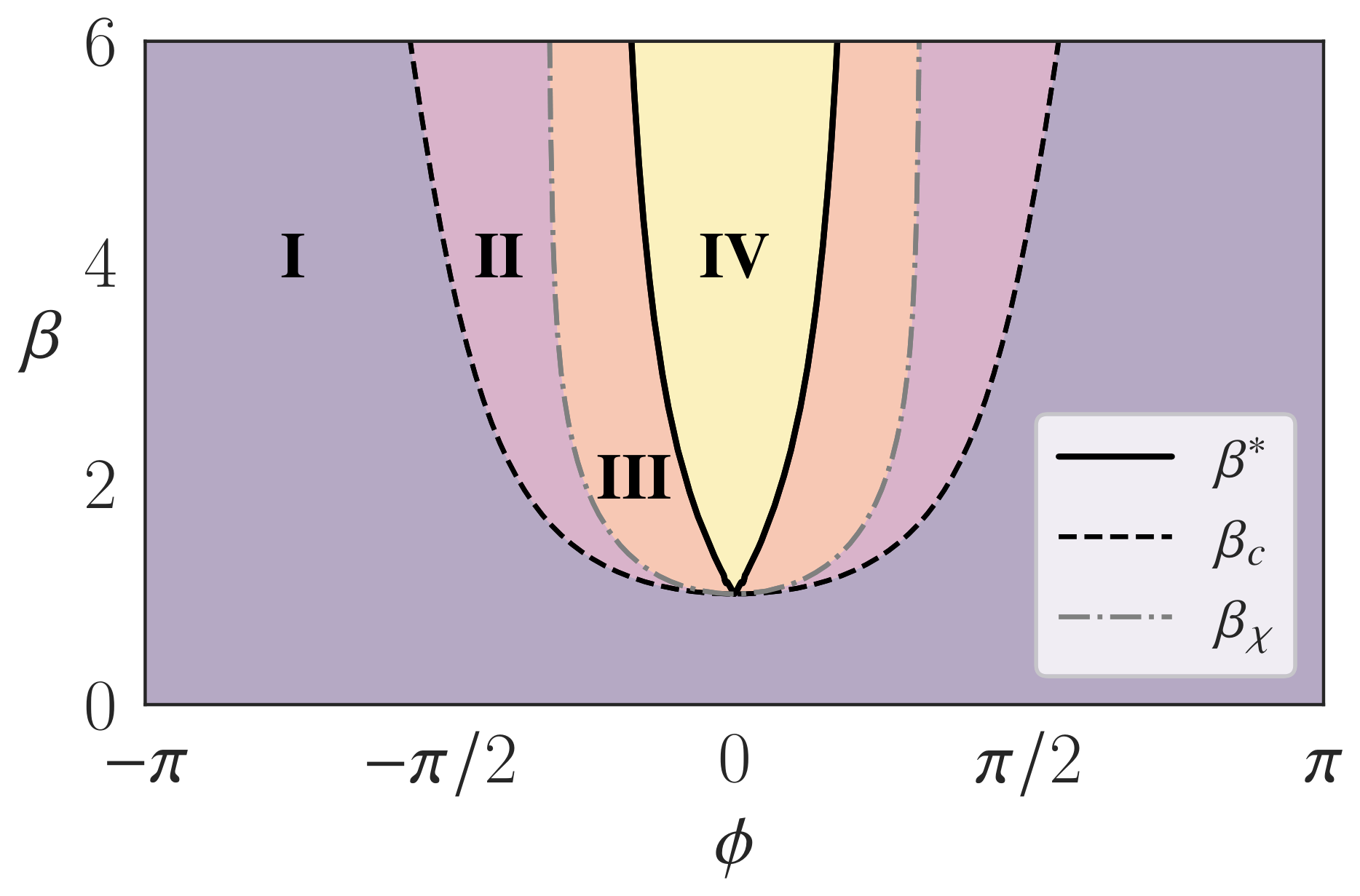
Phase diagram of two-pattern cycles at $\alpha=0$— We consider dynamical attractors constructed by matrices $\bm A = \bm \Omega_\phi$, being $\bm \Omega_\phi$ a $2\times 2$ rotation matrix with eigenvalues $e^{\pm \mathrm{i}\mkern1mu\phi}$. Encoding a single attractor set ($\alpha=0$), the dynamics converges to the mean field $\bm m_{t+1} = (1-\Delta) \bm m_t + \tfrac{\Delta}{2^M} \sum_{\bm \sigma} \bm \sigma \tanh[\beta \sigma^\top \bm \Omega_\phi \bm m_t]$. This system was studied by [28] at the $\Delta\to 0$ limit. The system converges to either one fixed point, four fixed points, or a single limit cycle, where $\phi$ controls the oscillation frequency (radians per update step) as $\omega = \arctan\big[\tfrac{\Delta\beta\sin\phi}{(1-\Delta)+\Delta\beta\cos\phi}\big]$.

We characterize the single-attractor phase structure of the system as a function of rotation angle $\phi$ and inverse temperature $\beta$ by computing three critical lines numerically. First, we calculate analytically a Hopf bifurcation by linearizing the overlap dynamics around $\bm m=0$, located at $\beta_c(\phi) = \Delta^{-1}(-(1-\Delta)\cos\phi + \sqrt{(1-\Delta)^2\cos^2!\phi + \Delta(2-\Delta)})$. Next, there is a heteroclinic bifurcation at $\beta^*(\phi)$ in which the cycle turns into four fixed points. We locate it using the bisection method for each fixed $\phi$ and finding numerically the value of $\beta$ where the limit cycle disappears. Finally, we calculate a third boundary $\beta_\chi$, characterized by the spectral radius of the response matrix $\bm\chi$ equal to $1$. We locate it numerically, also via the bisection method. After this point, the values of $R_{tt}$ diverge as $t\to\infty$, making the attractor unstable when $\alpha>0$.

The three lines partition the $(\phi,\beta)$ plane into four phases (Figure 4). Region I: $\beta<\beta_c$, paramagnetic phase with no pattern retrieval. Region II: $\beta_c<\beta<\beta_\chi$, unstable limit-cycle retrieval with $\lim_{t\to\infty} R_{tt} = \infty$, at any load $\alpha>0$. Region III: $\beta_\chi<\beta<\beta^*$, stable limit-cycle retrieval with bounded $R_{tt}$. Region *IV**: $\beta>\beta^$, fixed-point pattern retrieval.

{width=60%}

Calculation of the memory load capacity— For each inverse temperature $\beta$ and rotation angle $\phi$, we determine the critical capacity $\alpha_c(\beta)$ by bisection on $\alpha$. We initialize the network in a state aligned with the target patterns and evolve the mean-field equations for $\mathcal T$ time steps. The retrieval quality is measured by the root-mean-square overlap $|\bm m| = \sqrt{\langle |\bm m_t|^2 \rangle_t}$, averaged over the last $K$ time steps to filter transients. We define $\alpha_c$ as the largest $\alpha$ for which $|\bm m|$ exceeds a fraction $f$ of its value at $\alpha=0$, with $f=0.5$ throughout. The bisection terminates after at most $10$ iterations or when the bracketing interval falls below $10^{-4}$. For microscopic simulations, $\alpha_c$ is determined independently for each of $10$ random realizations of the disorder, and error bars report the sample standard deviation across trials.

Calculation of $\bm K, \bm R$ in the general case— Defining per-eigenvalue matrices $\bm G_\lambda = \sum_{n=0}^\infty \lambda^{n+1}\bm\chi^n$ and $\bm S_\lambda = \sum_{n,m=0}^\infty \lambda^{n+1}(\lambda^\ast)^{m+1}\bm\chi^n\bm q(\bm\chi^\top)^m$, so that

$ \bm K = \frac{1}{P}\sum_{r=1}^P \bm G_{\hat\lambda_r}, \qquad \bm R = \frac{1}{P}\sum_{r=1}^P \bm S_{\hat\lambda_r}, $

one obtains the recursive equations

$ \begin{aligned} \bm G_\lambda &= \lambda\left(\bm I + \bm\chi\bm G_\lambda\right), \quad\text{(a)} \ \bm S_\lambda &= |\lambda|^2\bm q + \lambda\bm\chi\bm S_\lambda + \lambda^\ast\bm S_\lambda\bm\chi^\top - |\lambda|^2\bm\chi\bm S_\lambda\bm\chi^\top, \quad\text{(b)} \end{aligned} $

which can be solved forward in time due to the strictly lower-triangular (causal) structure of $\bm\chi$. The special cases discussed in the main text follow by substituting the appropriate eigenvalue distributions.

Chaotic attractor search— The 4D orthogonal matrix $\bm{A}^\upsilon$ used for the chaotic attractor results was obtained via an island-model genetic algorithm at $\alpha=0$. The search space consists of the $2$ eigenvalue angles $\phi\in[0,\pi]$ and Givens plane angles $\psi_\mu\in[0,2\pi)$ parameterizing $\bm{A}\in\mathrm{SO}(M)$, together with $\beta$. The fitness function penalizes the leading Lyapunov exponent $\lambda_1$ falling below a threshold and the spectral radius of $\bm\chi$ exceeding unity, while rewarding positive $\lambda_1$. Each of the $10$ islands maintains an independent sub-population of 20 individuals evolved with Gaussian mutation with per-island adaptive step size $\sigma$, and elitism. Crossover samples each gene uniformly from an interval extending a fraction $0.3$ beyond the range spanned by the two parents. Every 10 generations, the two fittest individuals migrate along a ring topology. Mutation rates adapt between migrations: $\sigma$ shrinks upon improvement and grows upon stagnation, balancing exploitation and exploration across islands. The optimal solution found is

$ \begin{aligned} \bm{A}^\upsilon = \left[\begin{smallmatrix} 0.72192159 & 0.36388779 & 0.38903112 & 0.44166693 \ -0.42269013 & 0.72675866 & -0.35727641 & 0.40682732 \ -0.32417986 & 0.41701206 & 0.72090032 & -0.44867704 \ -0.44166693 & -0.40682732 & 0.44867704 & 0.66189936 \end{smallmatrix}\right], \end{aligned} $

at $\beta = 14.7329$, with leading Lyapunov exponents $\lambda_1\approx 0.032$, $\lambda_2\approx -0.001$.

References

Section Summary: This reference list compiles key scientific works on brain rhythms, such as theta and gamma oscillations in the hippocampus, alongside foundational studies of neural network models for memory storage and sequence processing. It includes classic papers on attractor networks like the Hopfield model, along with more recent research on nonreciprocal interactions, dynamical stability, and capacity limits in complex neural systems. The list also points to related books, mathematical derivations, and a code repository for exploring these ideas.

[1] Colgin, Laura Lee (2016). Rhythms of the hippocampal network. Nat. Rev. Neurosci.. 17(4). pp. 239–249. doi:10.1038/nrn.2016.21.

[2] Buzsáki, György and Vöröslakos, Mihály (2023). Brain rhythms have come of age. Neuron. 111(7). pp. 922–926. doi:10.1016/j.neuron.2023.03.018.

[3] Buzsáki, György (2006). Rhythms of the Brain. Oxford University Press.

[4] Wang, Xiao-Jing (2010). Neurophysiological and computational principles of cortical rhythms in cognition. Physiol. Rev.. 90. pp. 1195–1268. doi:10.1152/physrev.00035.2008.

[5] Lisman, John E. and Jensen, Ole (2013). The Theta–Gamma Neural Code. Neuron. 77(6). pp. 1002–1016. doi:10.1016/j.neuron.2013.03.007.

[6] Amit, Daniel J. (1989). Modeling Brain Function: The World of Attractor Neural Networks. Cambridge University Press.

[7] Coolen et al. (2005). Theory of Neural Information Processing Systems. Oxford University Press.

[8] Hopfield, John J. (1982). Neural networks and physical systems with emergent collective computational abilities. Proc. Natl. Acad. Sci. U.S.A.. 79(8). pp. 2554–2558. doi:10.1073/pnas.79.8.2554.

[9] Amit et al. (1985). Storing infinite numbers of patterns in a spin-glass model of neural networks. Phys. Rev. Lett.. 55(14). pp. 1530–1533. doi:10.1103/PhysRevLett.55.1530.

[10] Amari, Shun-Ichi (1972). Learning patterns and pattern sequences by self-organizing nets of threshold elements. IEEE Trans. Comput.. C-21(11). pp. 1197–1206. doi:10.1109/T-C.1972.223477.

[11] Sompolinsky, Haim and Kanter, Ido (1986). Temporal association in asymmetric neural networks. Phys. Rev. Lett.. 57(22). pp. 2861–2864. doi:10.1103/PhysRevLett.57.2861.

[12] Kleinfeld, David (1986). Sequential state generation by model neural networks. Proc. Natl. Acad. Sci. U.S.A.. 83(24). pp. 9469–9473. doi:10.1073/pnas.83.24.9469.

[13] Kleinfeld, David and Sompolinsky, Haim (1988). Associative neural network model for the generation of temporal patterns: Theory and application to central pattern generators. Biophys. J.. 54(6). pp. 1039–1051. doi:10.1016/S0006-3495(88)83041-8.

[14] Gutfreund, H. and Mézard, M. (1988). Processing of temporal sequences in neural networks. Phys. Rev. Lett.. 61(2). pp. 235–238. doi:10.1103/PhysRevLett.61.235.

[15] Avni et al. (2025). Nonreciprocal Ising Model. Phys. Rev. Lett.. 134. pp. 117103. doi:10.1103/PhysRevLett.134.117103.

[16] Avni et al. (2025). Dynamical phase transitions in the nonreciprocal Ising model. Phys. Rev. E. 111. pp. 034124. doi:10.1103/PhysRevE.111.034124.

[17] Düring et al. (1998). Phase diagram and storage capacity of sequence processing neural networks. J. Phys. A: Math. Gen.. 31(43). pp. 8607–8621. doi:10.1088/0305-4470/31/43/005.

[18] Kawamura, Masaki and Okada, Masato (2002). Transient dynamics for sequence processing neural networks. J. Phys. A: Math. Gen.. 35(2). pp. 253–266. doi:10.1088/0305-4470/35/2/306.

[19] Derrida et al. (1987). An exactly solvable asymmetric neural network model. Europhys. Lett.. 4(2). pp. 167–173. doi:10.1209/0295-5075/4/2/007.

[20] Derrida, B. and Nadal, J.-P. (1987). Learning and forgetting on asymmetric, diluted neural networks. J. Stat. Phys.. 49. pp. 993–1009. doi:10.1007/BF01017556.

[21] Crisanti, A. and Sompolinsky, H. (1988). Dynamics of spin systems with randomly asymmetric bonds: Ising spins and Glauber dynamics. Phys. Rev. A. 37. pp. 4865. doi:10.1103/PhysRevA.37.4865.

[22] Schlag et al. (2021). Linear Transformers Are Secretly Fast Weight Programmers. In Proceedings of the 38th International Conference on Machine Learning. pp. 9355–9366.

[23] Lucibello, Carlo and Mézard, Marc (2024). Exponential Capacity of Dense Associative Memories. Phys. Rev. Lett.. 132(7). pp. 077301. doi:10.1103/PhysRevLett.132.077301.

[24] Agliari et al. (2026). Exponential Capacity in Multilayer Hetero-Associative Neural Networks. doi:10.48550/arXiv.2607.29554. arXiv:2607.29554.

[25] Sommers, H.-J. (1987). Path-Integral Approach to Ising Spin-Glass Dynamics. Phys. Rev. Lett.. 58. pp. 1268–1271. doi:10.1103/PhysRevLett.58.1268.

[26] See Supplemental Material at [URL will be inserted by publisher] for detailed derivations of the generating functional, quenched disorder average, saddle-point equations, and mean-field dynamical equations..

[27] Eissfeller, H. and Opper, M. (1992). New method for studying the dynamics of disordered spin systems without finite-size effects. Phys. Rev. Lett.. 68(13). pp. 2094–2097. doi:10.1103/PhysRevLett.68.2094.

[28] Xue et al. (2025). Critical dynamics and cyclic memory retrieval in non-reciprocal Hopfield networks. SciPost Phys.. 19(4). pp. 100. doi:10.21468/SciPostPhys.19.4.100.

[29] Penttonen, Markku and Buzsáki, György (2003). Natural logarithmic relationship between brain oscillators. Thalamus Relat. Syst.. 2(2). pp. 145–152. doi:10.1016/S1472-9288(03)00007-4.

[30] Colgin et al. (2009). Frequency of gamma oscillations routes flow of information in the hippocampus. Nature. 462. pp. 353–357. doi:10.1038/nature08573.

[31] May, Robert M. (1972). Will a Large Complex System be Stable?. Nature. 238. pp. 413–414. doi:10.1038/238413a0.

[32] May, Robert M. (1973). Stability and Complexity in Model Ecosystems. Princeton University Press.

[33] Hutt et al. (2023). Intrinsic neural diversity quenches the dynamic volatility of neural networks. Proc. Natl. Acad. Sci. U.S.A.. 120(28). pp. e2218841120. doi:10.1073/pnas.2218841120.

[34] Hatton et al. (2024). Diversity begets stability: Sublinear growth and competitive coexistence across ecosystems. Science. 383(6688). pp. eadg8488. doi:10.1126/science.adg8488.

[35] Aguilera, Miguel (2026). Storing Infinite Dynamical Attractors in Nonreciprocal Associative Neural Networks: Code repository. https://github.com/MiguelAguilera/DynamicalMemoryCapacity.