Self-Improving Language Models with Bidirectional Evolutionary Search

Guowei Xu$^{1}$ Zhenting Qi$^{1}$ Huangyuan Su$^{1}$ Weirui Ye$^{2}$ Himabindu Lakkaraju$^{1}$ Sham M. Kakade$^{1}$ Yilun Du$^{1}$
$^{1}$ Harvard University $^{2}$ MIT

Abstract

Search has been proposed as an effective method for self-improving language models and agentic systems, both for post-training sample generation and for inference. However, widely used methods such as best-of-N sampling and tree search face two fundamental limitations: they are guided by sparse verification signals, and they construct candidates primarily through autoregressive expansion, restricting exploration to regions with substantial model probability mass. To address these, we propose Bidirectional Evolutionary Search (BES), a search framework that couples forward candidate evolution with backward goal decomposition. In the forward search, BES augments standard expansion with evolution operators that recombine partial trajectories to generate candidates that are difficult to obtain from a single model rollout. In the backward search, BES recursively decomposes the original task into checkable sub-goals, producing dense intermediate feedback that guides forward search. We provide theoretical motivation showing that candidates generated by expansion-only search are confined to a narrow entropy shell while evolutionary operators can escape it, and that backward search can exponentially reduce the number of required samples to find a correct answer. Experiments show that on challenging post-training tasks where mainstream post-training algorithms fail to improve, BES enables consistent gains, and on three open problem solving benchmarks at inference time, BES outperforms existing open-source frameworks in both average and best-case performance. Code and trained models are available at https://github.com/Embodied-Minds-Lab/BES.

Preprint.

Executive Summary: BES is a new search framework for improving the quality of outputs from large language models and agent systems. Current sampling methods such as best-of-N and tree search rely on sparse binary feedback and generate candidates only through sequential model rollouts. These constraints make it hard to discover high-quality solutions on difficult problems, limiting both post-training self-improvement and test-time performance gains.

The work introduces Bidirectional Evolutionary Search to overcome these limitations. Forward search augments standard expansion with four evolution operators—combination, deletion, translocation, and crossover—that recombine useful segments from different trajectories. Backward search recursively decomposes the original task into fine-grained, checkable sub-goals, supplying dense intermediate scores that guide candidate selection. The approach was evaluated on post-training for logical and multi-hop reasoning tasks, and on three open optimization benchmarks at inference time, using models up to 8 billion parameters and GPT-5.

Experiments show that BES produces meaningful gains where mainstream post-training methods such as GRPO, MaxRL, and Tree-GRPO deliver little or no improvement. On the MuSiQue multi-hop benchmark it raised accuracy by 3.0 percentage points on the 3B model and 3.8 points on the 8B model, while also increasing the number of valid search actions. At inference, BES outperformed three established open-source evolutionary frameworks on every open problem, achieved lower variance across runs, and required only modest additional API cost.

These results indicate that recombination beyond a single model’s output distribution, combined with structured sub-goal feedback, can unlock training and inference gains on frontier-level problems. The added overhead remains limited—roughly 30 percent more wall-clock time than tree search baselines—while delivering substantially stronger signals for downstream learning.

Organizations seeking stronger reasoning performance should consider integrating BES into post-training pipelines for hard reasoning domains and as an inference-time wrapper on open-ended tasks. Further validation on larger models, tasks without clear objective verifiers, and subjective domains would strengthen deployment decisions. The main limitations are dependence on reliable reward signals and the policy’s ability to perform goal decomposition; results on models larger than 8B remain to be confirmed.

1. Introduction

Section Summary: Large language models can tackle difficult reasoning tasks, but finding the best answers through sampling remains challenging, especially on frontier problems. Existing approaches like best-of-N sampling and tree search often provide only weak feedback and tend to stay within the model's familiar output patterns, limiting their ability to discover rare correct solutions. The paper introduces Bidirectional Evolutionary Search, which combines forward and backward exploration with biology-inspired operators to recombine and refine responses, yielding stronger results in both model training and inference across reasoning benchmarks.

Large language models (LLMs) and agentic systems have demonstrated remarkable capabilities on complex reasoning problems ([1, 2, 3]). They can even solve open problems across mathematical and scientific domains ([4, 5]) and surpass the best human performance on tasks such as code generation ([6, 7]). In this context, the question of how to do better sampling from LLMs and agentic systems is of critical importance ([8]). This is particularly significant for problems at the frontier of model capability, where naive sampling methods may require too many samples to obtain a correct answer or may simply fail ([9, 10]). At training time, higher-quality samples enable more effective post-training and self-improvement ([11, 12]); at inference time, they serve as a natural mechanism for test-time scaling ([13, 14, 15]), which can further push the boundary of what models can achieve.

Currently, the two dominant sampling methods in post-training, self-improvement, and inference for LLMs and agentic systems are best-of-N sampling and tree search. Best-of-N sampling is simple and efficient. For problems of moderate difficulty, it typically suffices to find high-quality responses and is therefore widely adopted in post-training algorithms such as GRPO ([3]) and its variants ([16]), while also serving as a strong baseline for inference. Tree search methods such as beam search and Monte Carlo Tree Search ([17]) can discover better responses more sample-efficiently than best-of-N on harder problems. For example, Tree-GRPO leverages tree search for sample generation during post-training ([18]), and Tree of Thoughts explores multiple reasoning paths at inference time ([19]).

However, both methods share two fundamental limitations. (1) The verification signal to guide the search is sparse. Effective search depends critically on the accuracy and granularity of the verifier, yet in common settings such as RLVR post-training, verifiers typically provide only binary or coarse-grained feedback. (2) They struggle to generate candidates beyond the model's own distribution. They construct candidates by auto-regressively extending responses. This confines candidates to the support of the model's own distribution ([20]), making it difficult to reach low-probability regions where correct solutions often reside on hard problems.

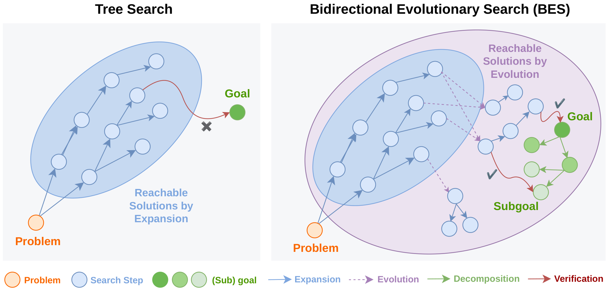
To address these two limitations, we propose Bidirectional Evolutionary Search (BES). First, to tackle the sparsity of verification signals, we introduce bidirectional search: the forward search seeks better candidate solutions, while the backward search discovers finer-grained sub-goals to verify them. Second, to generate candidates beyond the model's own distribution, we draw inspiration from evolutionary biology. For much of the history of life, organisms reproduced asexually. Each offspring was a direct extension of its parent, and beneficial mutations arising independently in different individuals could never be combined ([21]). Sexual reproduction fundamentally changed this through chromosomal recombination: gene segments from different lineages are spliced together to produce novel combinations that neither parent possessed ([22]). Analogously, in our setting, rather than only extending responses auto-regressively, we introduce four evolution operators: combination, translocation, deletion, and crossover. Combination, translocation, and crossover merge the strengths of two distinct responses in different ways to construct a new candidate, while deletion removes the least sound segment from a response. We theoretically prove that responses generated by expansion-only search are confined to a narrow entropy shell, while evolution operators can escape it.

We evaluate BES on both post-training and inference across LLM and agent settings. For post-training, we test on challenging logical reasoning and multi-hop reasoning tasks where mainstream post-training algorithms such as GRPO ([3]), MaxRL ([23]), and Tree-GRPO ([18]) struggle to find sufficient high-quality training samples and consequently fail to improve or even degrade from the base model. In contrast, BES consistently discovers effective training samples, enabling meaningful improvements where these baselines nearly fail. For inference, we test on three open problem solving benchmarks, where BES discovers more stable and higher-quality solutions compared to all existing open-source frameworks, including OpenEvolve ([24]), GEPA ([25]), and ShinkaEvolve ([15]). We also provide ablation studies validating the contribution of each component, case studies visualizing our search process, and cost analysis comparing the wall-clock time and API cost of BES against baselines.

2. Preliminaries

Section Summary: The section introduces reasoning tasks defined by a problem statement and a verifier that scores candidate solutions on a scale from zero to one. The central goal is to generate a high-scoring final answer under a generative policy such as a language model, yet directly locating the single best solution is intractable because such answers are typically very rare under the model’s own distribution. Practical methods therefore approximate the optimum by sampling many independent candidates and retaining the highest-scoring one, or by using tree-search procedures that expand promising partial solutions step by step.

We consider reasoning problems of the form $\mathcal{T} = (x, V), $ where $x$ is a problem description (e.g. a math question) and $V(x, y) \in [0, 1]$ is a verifier that assigns a score measuring how well a trajectory $y$ solves the problem $x$.

Given a policy $\pi_\theta(\cdot\mid x)$ (e.g. an LLM that generates reasoning traces, or an agent that interacts with an environment through a sequence of actions), our goal is to produce a terminal response $y$ that maximizes the verifier score. Let $\mathcal{Y}_{\mathrm{term}}(x)$ denote the set of valid terminal responses under the task specification and resource budget. We write the target as

$ y^{\star}(x) ;\in; \operatorname*{arg, max}{y\in\mathcal{Y}{term}(x)} V(x, y).\tag{1} $

Finding $y^{\star}$ is important in both training and inference. During training, high-quality candidates can facilitate post-training or iterative self-improvement. During inference, $y^{\star}$ is the response we seek.

The challenge is that the maximization in Equation 1 is intractable: on hard problems, the probability mass that $\pi_\theta$ assigns to correct trajectories can be extremely small. Practical algorithms therefore approximate $y^{\star}$ by searching over a set of candidates. We introduce two common methods below.

Best-of- $N$ sampling. The simplest approach is to draw $N$ independent trajectories and return the one with the highest verifier score. Formally, let $y^{(1)}, \dots, y^{(N)} \overset{\text{i.i.d.}}{\sim} \pi_\theta(\cdot \mid x)$. The method returns $ y^{\mathrm{BoN}} ;=; \operatorname*{arg, max}{y \in {y^{(1)}, \dots, y^{(N)}}} V(x, y) $. Best-of- $N$ is parallel and requires no structural knowledge of the problem. Its effectiveness, however, is bounded by the finite-sample coverage of $\pi\theta$: all $N$ trajectories are drawn from the same distribution, so if the optimal trajectory lies in a region with very small policy mass, increasing $N$ gives only linear coverage improvement.

Tree search. Tree-search methods exploit the sequential structure of a trajectory. A trajectory is decomposed into steps (e.g. tokens, reasoning segments, or agent actions), and the search maintains a tree whose nodes are partial trajectories and whose edges correspond to appending a step. Branches are selected and extended according to a heuristic value so that compute is concentrated on prefixes that look promising. Classic methods include beam search, best-first search, and Monte Carlo Tree Search ([17]); recent work applies these ideas to LLM and agent reasoning ([19, 18]). Tree search can be more sample-efficient than best-of- $N$ when the per-step signal is informative, but it still materializes terminal candidates one lineage at a time through sequential extension.

3. BES: Bidirectional Evolutionary Search

Section Summary: BES is a search method that alternates between two linked processes to solve complex problems more effectively than ordinary step-by-step generation. In the forward direction, it grows and reshapes collections of partial solutions by adding new steps and by mixing, shortening, or swapping pieces from different candidates, allowing combinations that a single straight-line attempt would rarely produce. The backward process repeatedly breaks the original goal into smaller sub-goals, then scores each partial solution by how many of those sub-goals it has already satisfied, supplying steady guidance that helps the forward process favor promising directions.

BES performs a bidirectional evolutionary search that alternates between two coupled processes: a forward search that seeks better candidates, and a backward search that decomposes the problem into fine-grained sub-goals to evaluate each forward node. The forward search not only extends trajectories but also recombines parts of different candidates, producing solutions that no single rollout from $\pi_\theta$ would likely reach. The backward search provides dense and interpretable scores for partial trajectories, guiding the forward search toward promising candidates. In practice, one backward search step is performed after every several forward search steps. The full pseudocode is given in Appendix A, and a case study illustrating the search process is provided in Appendix E.

3.1 Forward Search: Expanding the Reachable Solution Space

We represent each candidate partial trajectory as a node $n=(y_1, \dots, y_{t})$, where $y_i$ denotes the $i$-th step (e.g. a reasoning segment or an action). The search maintains a candidate set $\mathcal{P}$ of such nodes, and at each search step applies one of two types of operators, expansion or evolution, to produce a child node $n'$, which is scored by the backward search (Section 3.2) and added to $\mathcal{P}$.

Expansion. Expansion extends a parent node by sampling new steps. Given $n=(y_1, \dots, y_{t})$, we sample a step count $K\sim\mathrm{Uniform}{1, \dots, K_{\max}}$ and draw up to $K$ new steps from $\pi_\theta$:

$ y_{t+k}, \sim, \pi_\theta\bigl(\cdot\mid x\oplus y_1\oplus\cdot s\oplus y_{t+k-1}\bigr), \qquad k=1, \dots, K,\tag{2} $

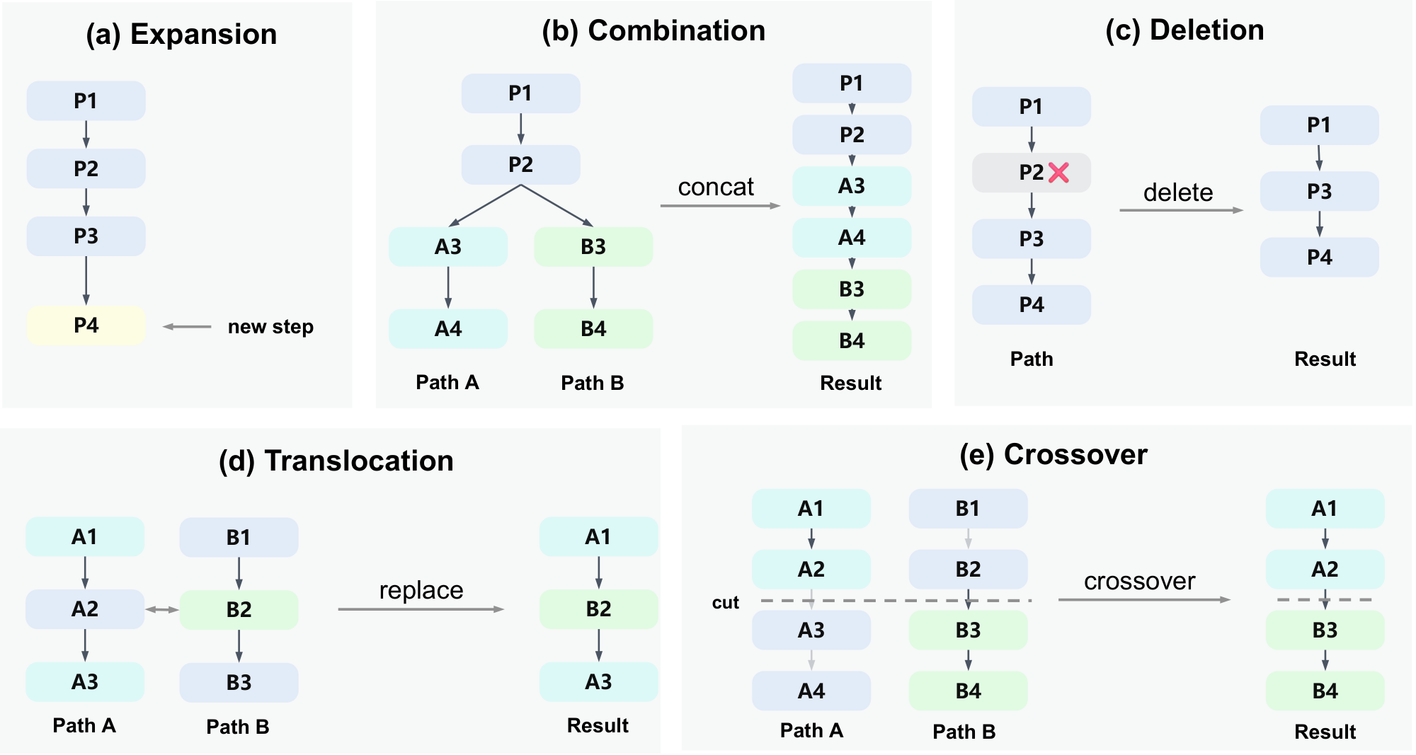
Evolution. A key limitation of expansion alone is that each candidate is built by sequentially extending a single trajectory, so it cannot combine useful parts from different candidates. Evolution operators overcome this by editing and recombining existing trajectories. As illustrated in Figure 2, we define four operators inspired by biological evolution: (i) Combination merges two trajectories by concatenating their suffixes beyond a shared prefix; (ii) Deletion removes one interior step, producing a shorter candidate; (iii) Translocation transplants a single step from one trajectory into another; and (iv) Crossover splices the prefix of one trajectory onto the tail of another. Formal definitions are provided in Appendix B. Together, these four evolution operators allow the search to restructure, condense, and recombine existing trajectories. As with mutations in nature, evolution operations are not guaranteed to produce better candidates. However, the value of evolution lies in generating diverse candidates: even if only a small fraction turn out to be improvements, that is sufficient for the search to make progress. Here, the four evolution operators are defined as direct edits on the step sequence. In settings where direct concatenation is not well-defined, the evolution operators can alternatively be implemented by prompting the policy model.

At each forward search step, we select among the operators with fixed probabilities. All operators require selecting one or two parent nodes from $\mathcal{P}$. Let $\mathcal{C}_t$ be the set of eligible non-terminal members of $\mathcal{P}$ at step $t$. For single-parent operators (expansion, deletion), we sample the parent from a Boltzmann distribution over backward score $s(n)$ Equation (5):

$ \Pr\bigl[n\mid\mathcal{C}t\bigr] ;=;\frac{\exp(\tilde{s}(n)/\tau_t)} {\sum{n'\in\mathcal{C}_t}\exp(\tilde{s}(n')/\tau_t)}, \qquad \tilde{s}(n) ;=; s(n) + \lambda\cdot\mathbf{1}!\bigl[\deg(n)=0\bigr],\tag{3} $

where $\tau_t>0$, $\deg(n)$ is the number of children of $n$ in $\mathcal{P}$, and the indicator term adds a small constant bonus $\lambda$ (we use $\lambda=0.1$) to candidates that have not yet been selected as parents, giving unexplored nodes a higher chance of being expanded.

For two-parent operators (combination, translocation, crossover), we select a pair of parent nodes $(n_a, n_b)$ from $\mathcal{C}_t$. We calculate a pair score $s(n_a, n_b)$ Equation (6) that favors complementary parents whose strengths cover different parts of the problem. The pair is then drawn from the analogous Boltzmann distribution:

$ \Pr[(n_a, n_b) \mid \mathcal{C}t] ;=;\frac{\exp(s(n_a, n_b)/\tau_t)} {\sum{n_a, n_b\in\mathcal{C}_t}\exp(s(n_a, n_b)/\tau_t)}.\tag{4} $

The temperature $\tau_t$ is annealed linearly from an initial value $\tau_0$ to a final value $\tau_{\mathrm{end}}<\tau_0$ over the search budget, gradually shifting from exploration to exploitation.

3.2 Backward Search: Better Verification through Goal Decomposition

While the verifier $V$ provides a score for each node in the forward search, this signal is relatively sparse. Backward search addresses this by decomposing the problem into a tree of fine-grained sub-goals. Each forward node is then scored against this tree: the more sub-goals a candidate trajectory has addressed, the higher its score. This gives the forward search a dense, informative signal to select promising candidates, even when none of them have fully solved the problem yet.

Below we describe how the backward search is constructed. Starting from the top-level goal $g_{\texttt{root}}$ (i.e. solving the entire problem), the policy $\pi_\theta$ is prompted to break each goal into finer sub-goals, producing a rooted backward goal tree. Each goal $g$ on the tree can be recursively split into children $\mathrm{ch}(g)$ (finer sub-goals), and every $g$ comes with a verifier $V_g(x, n) \in [0, 1]$ that tests how well a candidate node $n$ addresses the sub-goal $g$ on problem $x$. For the top-level goal, $V_{g_{\texttt{root}}} = V$ (the verifier of the original problem). This decomposition is re-invoked every $K$ forward search steps: at each invocation, we select a leaf sub-goal that no current candidate fully satisfies and prompt $\pi_\theta$ to split it into finer sub-goals. After that, all existing forward nodes are re-scored. The verifiers are task-dependent and can be instantiated as rule-based checkers, test-case code executors, embedding similarity models, or LLM judgers. We describe the verifiers used in each experiment in Appendix D.

For example, consider the problem "Compute $\frac{(4+6)\times 3}{2} - 5$." The backward search can produce the following goal tree:

:::: .figure

for tree={ grow'=0, anchor=west, child anchor=west, parent anchor=east, l sep=12mm, s sep=4mm, edge=->, >=latex, font=, } [$g_{\texttt{root}}$: compute $\frac{(4+6)\times 3}2 - 5$ [$g_1$: compute $(4+6)\times 3$ [$g_1.1$: compute $4+6$] [$g_1.2$: #1 multiply by $3$]] [$g_2$: #1 divide by $2$] [$g_3$: #2 subtract $5$]]

::::

For a candidate node $n$ from the forward search (Section 3.1) and a sub-goal $g$, define the sub-goal score

$ s(n, g) ;=; \alpha\cdot V_g(x, n) ;+;(1-\alpha)\cdot\frac{1}{|ch(g)|} \sum_{g'\in ch(g)} s(n, g'),\tag{5} $

where $\alpha\in[0, 1]$ balances the contribution of coarser parent goals and finer-grained sub-goals to the overall score. For leaf sub-goals ($\mathrm{ch}(g)=\emptyset$), we set $s(n, g)=V_g(x, n)$. If a goal is already fully satisfied ($V_g(x, n)=1$), we short-circuit to $s(n, g)=1$ without evaluating its children. The overall score is $s(n)\triangleq s(n, g_{\texttt{root}})$.

For two candidate nodes $n_a$ and $n_b$, we further define a pair score that measures their joint coverage of the goal tree. Replacing each sub-goal verifier with the maximum of the two parents' scores gives

$ s(n_a, n_b, g) ;=; \alpha\cdot \max{V_g(x, n_a), , V_g(x, n_b)} ;+;(1-\alpha)\cdot\frac{1}{|ch(g)|} \sum_{g'\in ch(g)} s(n_a, n_b, g'),\tag{6} $

with $s(n_a, n_b)\triangleq s(n_a, n_b, g_{\texttt{root}})$. A sub-goal is considered covered if either parent addresses it, so the pair score favors complementary parents that cover different parts of the goal tree.

Applying this procedure to every node in the forward search tree yields a backward score for each node and a pair score for each pair of nodes, which directly drive node selection in the forward search.

3.3 Using BES for Post-Training and Inference

Post-Training. BES replaces the sample-generation stage of post-training. Given a training problem, BES returns a set of high-quality trajectories from the forward search candidate set $\mathcal{P}$. These trajectories are then used as training data for post-training algorithms, replacing the candidates that would otherwise be obtained from i.i.d. rollouts. Because BES can find correct solutions that single rollouts rarely reach, it provides stronger training signal, especially on hard problems.

Inference. At inference time, BES runs on open problems with a fixed compute budget, and the terminal trajectory with the highest score is returned as the final answer.

4. Theoretical Motivations

Section Summary: Evolution operators confer a fundamental advantage over standard expansion-only search because they can break the statistical dependencies between segments of a trajectory and thereby produce candidates whose likelihood under the original policy lies well outside the narrow high-probability “entropy shell” to which ordinary rollouts are confined. Under mild assumptions on bounded surprise, decaying dependence, and linear growth of block correlations, the expected log-probability of an evolved trajectory exceeds the shell boundary by a term proportional to total correlation, so that a non-vanishing fraction of such candidates escape the typical set. Bidirectional search complements this enlargement of the candidate space by turning discovered sub-goals into independent early-warning signals; the resulting reduction in the number of trials needed to reach a solution is exponential in the number of sub-goals relative to terminal-only verification.

4.1 Theoretical Motivation for Evolution Operators

We justify why evolution operators provide a fundamental advantage over expansion-only search. Specifically, we prove that expansion-only candidates are confined to a narrow entropy shell, while evolution operators can escape it. The full proof is given in Appendix C.1.

Fix a task $x$ and a step horizon $T$. A trajectory $Y = (y_1, \dots, y_T)$ is generated by the policy with probability $P(Y) = \prod_{t=1}^T P(y_t \mid y_{<t})$. Let $H_T = H_P(Y)$ denote the trajectory-level entropy. We partition the trajectory into $k$ contiguous blocks $U_1, \dots, U_k$. We make three assumptions on the policy. All of them are naturally satisfied in practice; see Appendix C.1.1 for a detailed discussion.

########## {caption="Assumption 1: Bounded per-step surprise"}

There exists $L<\infty$ such that for every reachable prefix and every step with positive probability, $-\log P(v\mid y_{<t})\le L$.

########## {caption="Assumption 2: Decaying step dependence"}

There exists a summable nonnegative sequence $(\beta_\ell){\ell\ge1}$ with $C\beta:=\sum_{\ell\ge1}\beta_\ell<\infty$ such that for every $s<t$, prefix $y_{<s}$, and two steps $v, v'$ at position $s$,

$ \begin{aligned} &\left| \mathbb{E}!\big[h_t(Y_{<t})\mid Y_{<s}=y_{<s}, Y_s=v\big]

\mathbb{E}!\big[h_t(Y_{<t})\mid Y_{<s}=y_{<s}, Y_s=v'\big] \right| \le \beta_{t-s}. \end{aligned} $

########## {caption="Assumption 3: Linear block total correlation"}

We partition the trajectory into $k \geq 2$ contiguous blocks $U_1, \dots, U_k$ at fixed boundaries $0 = s_0 < s_1 < \cdot s < s_k = T$. The block total correlation grows linearly in the horizon: $\sum_{j=1}^k H_P(U_j) - H_P(U_1, \ldots, U_k) \geq \gamma T$ for some constant $\gamma > 0$.

########## {caption="Theorem 4: Shell confinement and escape"}

Under Assumption 1–Assumption 3, define the typical set $A_\epsilon^{(T)}:={y:|-\log P(y)-H_T|\le\epsilon T}$.

(a) Shell confinement. Every trajectory $Y \sim P$ produced by expansion-only search satisfies $\Pr[Y \notin A_\epsilon^{(T)}] \leq \exp(-\Omega(T))$. That is, search is confined to a typical set of size at most $\exp(H_T + \epsilon T)$.

(b) Shell escape. Let $Q = \bigotimes_{j=1}^k P_j$ be the $k$-time evolution distribution. For any $\epsilon < \gamma$,

$ \mathbb{E}_Q[-\log P(\widetilde{Y})] ;\geq; H_T + \gamma T ;>; H_T + \epsilon T,\tag{7} $

so evolution candidates have expected log-probability strictly beyond the shell boundary. Moreover,

$ \Pr_Q!\left[\widetilde{Y} \in A_\epsilon^{(T)}\right] ;\leq; 1 - \frac{(\gamma - \epsilon)T}{LT - H_T - \epsilon T} ;<; 1,\tag{8} $

confirming that a positive fraction of evolution candidates escape the shell.

Proof sketch. We first establish that, with high probability, every policy rollout has log-probability close to $H_T$, confining expansion-only search to a thin entropy shell. We then show that evolution operators break inter-block dependence and result in increased surprise (Lemma 11). Generalizing to $k$-time evolution, the expected surprise exceeds $H_T$ by the block total correlation (Lemma 12), which is $\Omega(T)$ under Assumption 3, pushing evolution candidates outside the shell.

4.2 Theoretical Motivation for Bidirectional Search

The previous section shows that evolution operators can construct candidates beyond the policy's entropy shell. We now show that backward search makes this enlarged space efficiently searchable. The full proof is given in Appendix C.2.

Let the backward search produce $m$ leaf sub-goals ${g_1, \ldots, g_m}$. For a candidate trajectory $n$, define $C_i(n)=\mathbf{1}{V_{g_i}(x, n)=1}$. We assume that terminal success requires all leaf sub-goals: $V(x, n)=1 \Rightarrow C_i(n)=1, \ \forall i\in[m]$. For simplicity, suppose that for a fresh candidate $n$, the events ${C_i(n)=1}$ are independent with probabilities $\Pr[C_i(n)=1]=p_i$.

########## {caption="Theorem 5: Exponential advantage from backward sub-goal signals"}

Let $N$ candidates be sampled independently. Terminal-only search requires $N_{\mathrm{term}} = \Omega!\left(1 / \prod_{i=1}^m p_i\right)$ candidates to obtain constant success probability. By contrast, backward-guided bidirectional search requires only $N_{\mathrm{bidir}} = O!\left(p_{\min}^{-1}\log(m/\delta)\right)$, where $p_{\min}=\min_i p_i$, to collect evidence for all sub-goals with probability at least $1-\delta$. In the symmetric case $p_i=p$, the ratio is $N_{\mathrm{term}} / N_{\mathrm{bidir}} = \Omega!\left(p^{-(m-1)} / \log(m/\delta)\right)$, which is exponential in the number of sub-goals $m$.

5. Experiments

Section Summary: The experiments evaluate Bidirectional Evolutionary Search (BES) in two main settings: improving model training after initial fine-tuning and guiding the search for solutions during inference. In post-training tests on logical puzzles and multi-hop reasoning tasks, BES produced steady gains in accuracy and encouraged more effective problem-solving behavior compared with standard reinforcement methods like GRPO, which often stalled or degraded performance. During inference on open-ended challenges such as circle packing and point-placement problems, BES again outperformed existing evolutionary frameworks, delivering higher-quality solutions with greater consistency.

We evaluate BES on both post-training and inference across LLM and agent settings. For post-training, we consider Logical Reasoning (LLM) and Multi-Hop Reasoning (Agent). For inference, we consider three representative open problem solving benchmarks: Circle Packing (Square), Circle Packing (Rectangle), and the Heilbronn Convex problem. In each benchmark, we compare BES against commonly used baselines and show that BES consistently achieves better sampling.

5.1 Bidirectional Evolutionary Search for Post-Training

5.1.1 Logical Reasoning

For logical reasoning, we use the Knights-and-Knaves dataset ([26]). In this task, each puzzle involves a group of people who are either a knight or a knave, and the solver must deduce each one's identity.

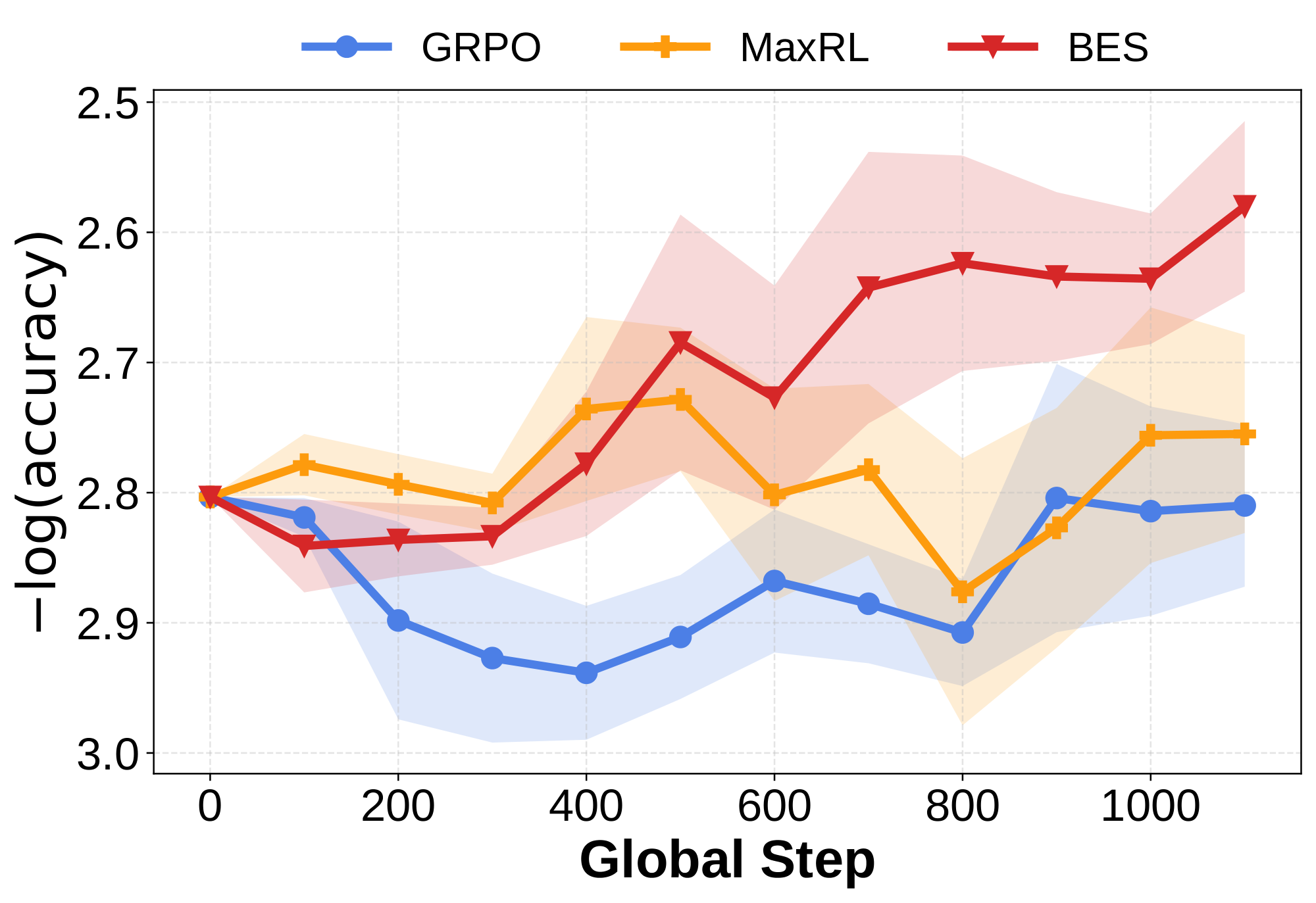
Baselines. We select two post-training algorithms, GRPO ([3]) and MaxRL ([23]), as baselines, as we apply BES on top of MaxRL. We note that BES is a sampling algorithm that is agnostic to the training method and can be applied on top of any post-training algorithm.

Training Setup. We use Gemma-3-1B-it ([27]) as the base model. To adapt the model to the Knights-and-Knaves benchmark, we first perform a cold start by fine-tuning on 1K SFT examples generated using the official data generation pipeline for 3 epochs, followed by 4 epochs of post-training on 5K problems, during which we compare the different methods on a 1.3K validation set. Detailed experimental configurations are provided in Appendix D.1.

Results. As shown in Figure 3, due to the difficulty of the training set, GRPO and MaxRL show little to no improvement during training, while BES steadily improves on the validation set throughout training, demonstrating that BES is more effective at discovering high-quality training samples.

5.1.2 Multi-Hop Reasoning

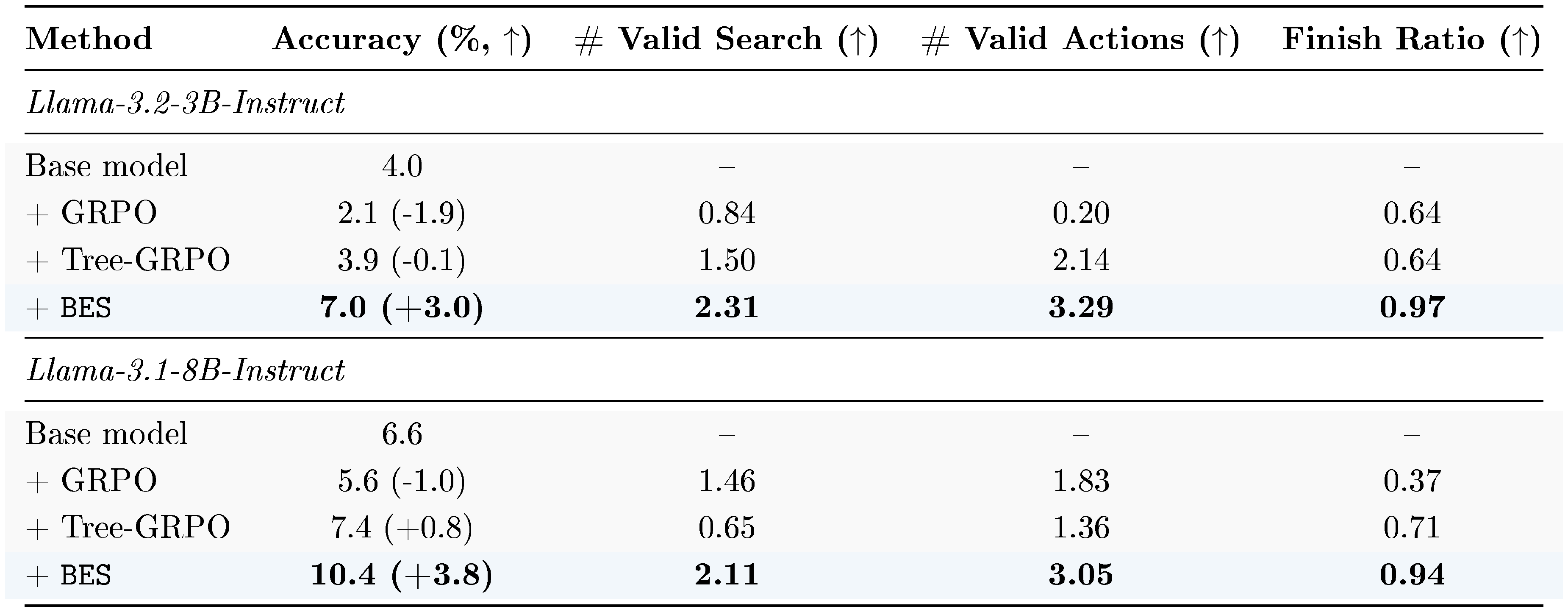
::: {caption="Table 1: Multi-hop reasoning post-training results on MuSiQue with Llama-3.2-3B-Instruct and Llama-3.1-8B-Instruct. We report accuracy, number of valid searches, number of valid actions, and finish ratio. Higher is better for all metrics. Bold denotes the best performing method per backbone."}

:::

For multi-hop reasoning, we use the MuSiQue dataset ([28]). In this task, the agent must answer complex questions that require retrieving and integrating information across multiple documents, where no single document contains the complete answer.

Baselines. We compare against GRPO ([3]) and Tree-GRPO ([18]), with the latter being the current state-of-the-art method for search agent post-training. We apply BES on top of GRPO.

Training Setup. We adopt the training setup of Tree-GRPO ([18]), using Llama-3.2-3B-Instruct and Llama-3.1-8B-Instruct ([29]) as base models. During the search process, the agent can perform multiple search actions before producing a final answer. Search results are provided by an offline Wikipedia server. We use the 3–4 hop solvable subset of the MuSiQue training set as our training data and train for 2 epochs, as additional epochs lead to training collapse. We evaluate on the full official MuSiQue validation set. Detailed configurations are provided in Appendix D.2.

Results. As shown in Table 1, GRPO consistently degrades from the base model on both scales, likely due to reward hacking where the model learns to skip search actions and guess directly, as reflected by its low number of valid searches. Tree-GRPO provides marginal improvement on the 8B model ($+0.8%$) but fails to improve the 3B model. In contrast, BES achieves substantial gains on both scales ($+3.0%$ on 3B, $+3.8%$ on 8B), outperforming all baselines by a wide margin. Beyond accuracy, BES also produces agents with significantly more valid search actions and higher finish ratios, indicating that the trained agents learn to actively search rather than randomly guessing.

5.2 Bidirectional Evolutionary Search for Inference

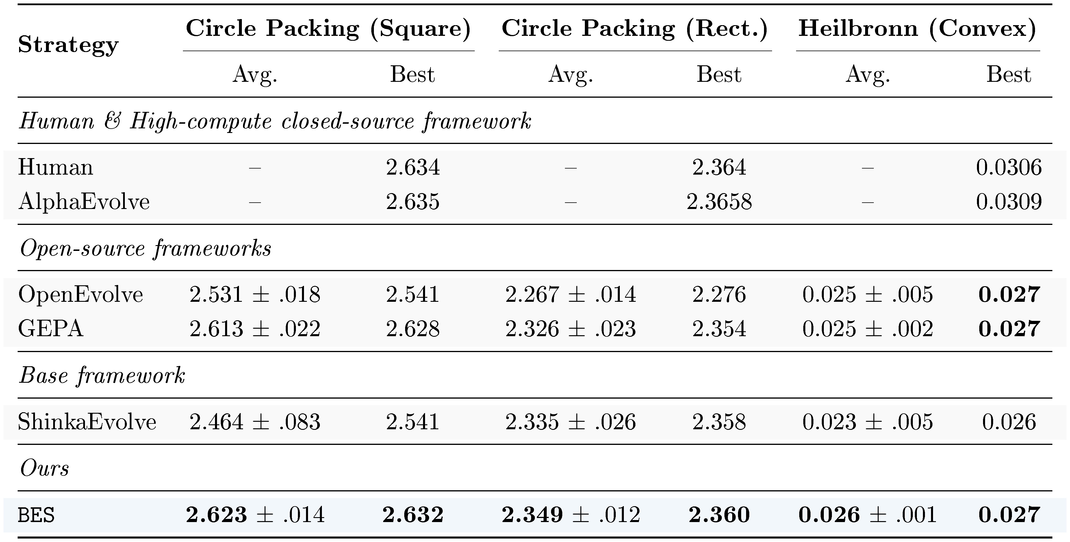
At inference time, we evaluate the ability of BES to solve open problems. Specifically, we consider three benchmarks: Circle Packing (Square), which seeks to pack $N$ circles into a unit square with maximum radius; Circle Packing (Rect), the analogous problem for a rectangular container; and Heilbronn (Convex), which seeks to place $N$ points in the unit square to maximize the minimum area of any convex polygon formed by subsets of the points.

::: {caption="Table 2: Open problem solving benchmarks with GPT-5 as the backbone model. We report Mean ± Std and Best objective values (↑). Bold denotes the best performing method."}

:::

Baselines. We compare against three open-source frameworks: OpenEvolve ([24]), GEPA ([25]), and ShinkaEvolve ([15]). All baseline results are taken from SkyDiscover ([30]), which uses the same backbone model, compute budget, and configuration as ours. We apply BES on top of ShinkaEvolve. For reference, we also include the results of human experts and AlphaEvolve ([4]), which is closed-source and uses significantly more compute than all other frameworks.

Setup. ShinkaEvolve maintains a population of candidate programs and iteratively proposes modifications. Since directly concatenating model outputs is not meaningful on this benchmark (where candidates are executable programs), we implement the evolution operators by prompting LLMs. We use GPT-5 as the backbone model. Detailed configurations are provided in Appendix D.3.

Results. As shown in Table 2, BES outperforms open-source frameworks on every benchmark. Notably, BES also exhibits much lower variance across runs than all baselines, indicating the search is more stable and reliable. In Appendix N, we list a summary of the best programs discovered by BES.

5.3 Ablation Study

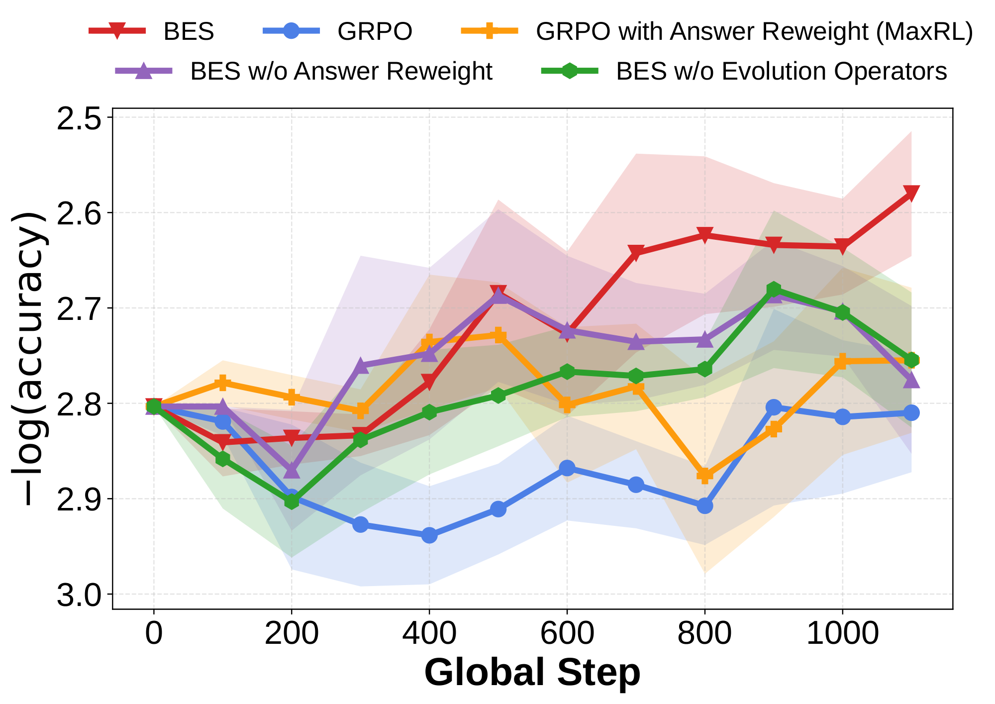
We conduct an ablation study on the Knights-and-Knaves benchmark. On this benchmark, BES combines bidirectional evolutionary search for discovering high-quality samples with MaxRL's answer reweighting for training. We therefore consider two ablations: (1) removing answer reweighting; and (2) removing the evolution operators to verify that both bidirectional search and evolution operators are necessary. As shown in Figure 4, both ablations underperform the full BES method, while still outperforming the GRPO and MaxRL baselines. This confirms the effectiveness of each component in our approach.

5.4 Cost Analysis

Post-Training. To evaluate the cost-effectiveness of BES, we compare the per-step wall-clock time and final accuracy across GRPO, Tree-GRPO, and BES when training Llama-3.2-3B-Instruct on the agentic search task. We report the median wall-clock time per step throughout the training process.

\begin{tabular}{lccc}
\toprule
\textbf{Method} & \textbf{Accuracy (\%)} & \textbf{# Valid Search} & \textbf{Walltime (s)} \\
\midrule
\rowcolor{cellbase} GRPO & 2.1 (-1.9) & 0.84 & 64 \\
\rowcolor{cellbase} Tree-GRPO & 3.9 (-0.1) & 1.50 & 240 \\
\rowcolor{tabband} \texttt{BES} & \textbf{7.0 (+3.0)} & \textbf{2.31} & 309 \\
\bottomrule
\end{tabular}

Notably, the low wall-clock time of GRPO is misleading: during training, GRPO quickly exhibits reward hacking, with the model learning to skip search actions and guess answers directly, as reflected by its low number of valid searches. In contrast, BES incurs less than 30% additional overhead compared to Tree-GRPO, while achieving significantly better performance across all metrics.

Inference. We compare the API cost of BES against ShinkaEvolve across all three open problem solving benchmarks. As shown in Table 4, BES achieves consistently higher average values while incurring modest additional API costs.

\begin{tabular}{lccccccccc}
\toprule
& \multicolumn{3}{c}{\textbf{Circle Packing (Sq.)}} & \multicolumn{3}{c}{\textbf{Circle Packing (Rect.)}} & \multicolumn{3}{c}{\textbf{Heilbronn (Convex)}} \\
\cmidrule(lr){2-4} \cmidrule(lr){5-7} \cmidrule(lr){8-10}
\textbf{Method} & Avg. & Best & Cost & Avg. & Best & Cost & Avg. & Best & Cost \\
\midrule
\rowcolor{cellbase} ShinkaEvolve & 2.464 & 2.541 & \$13.0 & 2.335 & 2.358 & \$11.9 & 0.023 & 0.026 & \$11.5 \\
\rowcolor{tabband} \texttt{BES} & \textbf{2.623} & \textbf{2.632} & \$18.6 & \textbf{2.349} & \textbf{2.360} & \$14.0 & \textbf{0.026} & \textbf{0.027} & \$13.7 \\
\bottomrule
\end{tabular}

6. Related Work

Section Summary: Recent research has explored how large language models can improve themselves by generating and filtering their own outputs for training or by using feedback at runtime, as seen in methods that refine reasoning or build reusable skills through exploration. A related line of work applies search techniques during both model training and inference, often expanding possible reasoning paths in tree-like structures or evolving populations of candidate solutions, though these approaches tend to remain limited by the model's existing tendencies and struggle to venture into truly novel territory. These modern techniques build on longstanding ideas from classical computer science, such as heuristic-guided graph search, branch pruning to eliminate weak options early, and population-based evolutionary algorithms.

Self-Improvement for LLM and Agent. A growing line of work studies how language models and agents can improve using their own outputs to self-evolve ([31, 32]). STaR ([11]) bootstraps reasoning by filtering correct rationales for fine-tuning, while Self-Refine ([33]) revises outputs at inference time through self-generated feedback. Self-Rewarding Language Models ([12]) use the model itself as a judge for preference optimization. In agentic settings, Reflexion ([34]) converts environmental feedback into verbal reflections, and Voyager ([35]) accumulates reusable skills through continual exploration. These methods typically refine individual trajectories or rely on the model to judge its own outputs. In contrast, BES treats self-improvement as a structured search problem, systematically discovering high-quality solutions that facilitate model self-improvement.

Search in LLM and Agent. Recent work applies search to both training and inference of LLMs and agents ([36, 37]). On the training side, tree-structured exploration provides richer supervision and finer-grained credit assignment than standard rollout-based methods. Tree-GRPO ([18]) and TreeRL ([38]) integrate tree search directly into reinforcement learning, while ReST-MCTS* ([39]), MCTS-DPO ([40]), and rStar-Math ([8]) use search to bootstrap higher-quality training data for self-improvement. On the inference side, Tree of Thoughts ([19]), Graph of Thoughts ([41]), and RAP ([42]) established reasoning as an explicit search problem by expanding chain-of-thought into tree-structured exploration ([43]). More recently, evolutionary approaches such as AlphaEvolve ([4]), ShinkaEvolve ([15]), and ThetaEvolve ([44]) tackle hard and even open problems ([45]) by maintaining candidate populations with LLM-driven mutations and external evaluation. However, these methods predominantly rely on tree search and thus struggle to explore beyond the policy's own distribution.

Classical Search Methods. The recent surge of search-based methods in LLMs and agents draws on a long history of classical search. In symbolic planning and graph search, algorithms such as A* ([46]) and bidirectional search introduced core principles including heuristic guidance, frontier expansion, and search-space reduction. Branch-and-bound methods ([47]), which prune subtrees whose bounds certify suboptimality, offer a natural analogy for modern methods that use verifiers to discard unpromising candidates early. Evolutionary methods, including genetic search ([48, 49]) and differential evolution ([50]), optimize by maintaining and iteratively refining candidate populations.

7. Conclusion

Section Summary: The paper introduces BES, a new search method designed to help large language models and AI agents solve complex problems more effectively. It works by evolving candidate solutions in a forward direction while also breaking problems down backward into smaller, verifiable steps that give clearer feedback along the way. Theoretical analysis and experiments on reasoning and open-ended tasks show that this bidirectional approach outperforms prior methods and offers a promising path toward self-improving AI systems.

In this paper, we present BES, a bidirectional evolutionary search framework that addresses two fundamental limitations of existing search methods for LLMs and agents: sparse verification signals and confined candidate generation. BES couples forward search, which evolves candidates through expansion and four evolution operators, with backward search, which recursively decomposes problems into verifiable sub-goals to provide dense intermediate feedback. We provide theoretical justification showing that candidates generated by expansion-only search are confined to a narrow entropy shell while evolution operators can escape it, and that backward sub-goal decomposition exponentially reduces the number of candidates needed to find a solution. Experiments on logical reasoning, multi-hop reasoning, and open problem solving demonstrate that BES consistently improves over strong baselines in both post-training and inference settings. We hope that BES provides useful insights for self-improving language models and agents.

Appendix

Section Summary: The appendix presents the complete pseudocode for the Bidirectional Evolutionary Search algorithm, including its main loop that alternates forward generation steps with backward scoring on a goal tree, plus procedures for sampling evolutionary operators, refining unsolved sub-goals, and recomputing scores. It also supplies formal mathematical definitions of the five operators (expansion, deletion, combination, translocation, and crossover) that recombine solution trajectories, followed by a theoretical discussion of why such recombination improves coverage over single-lineage search by leveraging measures of surprisal and conditional entropy.

etocdepthtag.tocappendix etocsettocstyle{

Appendix - Table of Contents

A. Pseudo Code

We provide the full pseudocode for BES below. Algorithm 1 describes the main loop, which alternates between forward search steps (Algorithm 2) and backward scoring (Algorithm 3). Every $K_{\mathrm{dec}}$ steps, the backward goal tree is refined by decomposing an unsolved leaf into finer sub-goals (Algorithm 4), after which all pool scores are recomputed under the updated tree.

```algorithm {caption="**Algorithm 1:** BES: Bidirectional Evolutionary Search" .numberLines startFrom="0"} Require: problem x, policy π(θ), verifier V, budget B, decomposition interval K(dec) Initialize G with root goal g₀; prompt π(θ) to decompose g₀ into initial sub-goals P ← (n₀) with n₀ = () // Empty root node for t = 0, 1, … while calls(t) < B do n' ← FORWARDSTEP(P, C(t), G, τ(t)) // Algorithm 2 s(n') ← BACKWARDSCORE(n', g₀, G) // Algorithm 3 P ← P cup (n') if (t+1) bmod K(dec) = 0 then G ← BACKWARDDECOMPOSE(x, G, P) // Algorithm 4 for n ∈ P // Recompute all scores under refined tree do s(n) ← BACKWARDSCORE(n, g₀, G) end for end if if n' is terminal ∧ V(x, n') = 1 then

**return** n'

end if end for return argmax(n ∈ P: terminal(n)) V(x, n)

Algorithm 2 details a single forward search step. An operator is sampled from the fixed distribution over the five operators. Single-parent operators (expansion and deletion) select a parent via Boltzmann selection based on backward scores; two-parent operators (combination, translocation, crossover) select a pair that maximizes joint sub-goal coverage.

```algorithm {caption="**Algorithm 2:**  $\textsc{ForwardStep}$: Forward Search Step" .numberLines startFrom="0"}
**Require:** pool P, eligible set C(t), goal tree G, temperature τ(t)
Sample operator o ∈ (expand, combine, delete, translocate, crossover) with fixed probabilities
**if** o ∈ (expand, delete) // Single-parent operators **then**
  Sample parent n from C(t) via Boltzmann selection (Eq. 3)
  **if** o = expand **then**
    Sample K ∼ Uniform(1, …, K(max))
    n' ← (y₁, …, y(t), y(t+1), …, y(t+K)) where y(t+k) ∼ π(θ)(· | x ⊕ y(1:t+k-1))
  **else**
    Sample ell ∼ Uniform(2, …, t-1); n' ← (y₁, …, y(ell-1), y(ell+1), …, y(t))
  **end if**
**else**
  Sample pair (n(a), n(b)) from C(t) via pair Boltzmann selection (Eq. 4)
  Compute shared prefix length s and suffixes σ(a), σ(b)
  **if** o = combine **then**
    n' ← y(a,1:s) ⊕ σ(a) ⊕ σ(b)
  **else if** o = translocate **then**
    Sample r, q; n' ← y(a,1:s) ⊕ σ(a)[1:r - 1] ⊕ (σ(b))_q ⊕ σ(a)[r + 1:m(a)]
  **else if** o = crossover **then**
    Sample i, j; n' ← y(a,1:s) ⊕ σ(a)[1:i] ⊕ σ(b)[j + 1:m(b)]
  **end if**
**end if**
**return** n'

Algorithm 3 computes the backward score for a candidate node by recursively traversing the sub-goal tree. If a sub-goal is fully satisfied, the score is 1; otherwise, the score blends the local verifier output with the average score over its children.

**Require:** candidate node n, sub-goal g, goal tree G
**if** V(g)(x, n) = 1 **then**

  **return** 1
**else if** ch(g) ≠ ∅ **then**

  **return** α · V(g)(x, n) + (1 - α) · 1/|ch(g)| ∑ over g' ∈ ch(g) BACKWARDSCORE(n, g', G)
**else**

  **return** V(g)(x, n)
**end if**

Algorithm 4 refines the goal tree by selecting a random unsolved leaf sub-goal and prompting the policy to decompose it into finer children, each equipped with its own local verifier.

**Require:** problem x, current goal tree G, pool P
L ← (g ∈ G : ch(g) = ∅ ∧ max(n ∈ P) V(g)(x, n) < 1) // Unsolved leaves
Sample g* uniformly from L
Prompt π(θ) to decompose g* into children (g'₁, …, g'(c)) with local verifiers (V(g)'₁, …, V(g)'(c))
ch(g*) ← (g'₁, …, g'(c)); add to G
**return** G

B. Formal Definitions of Evolution Operators

For two parents $n_a, n_b$, let $s=\max{\ell:y_{a, 1:\ell}=y_{b, 1:\ell}}$ denote their common-prefix length, and let $\sigma_a=(y_{a, s+1}, \dots, y_{a, t_a})$ and $\sigma_b=(y_{b, s+1}, \dots, y_{b, t_b})$ be their respective suffixes.

(i) Combination. $n' = y_{a, 1:s}, \oplus, \sigma_a, \oplus, \sigma_b$.

(ii) Deletion. $n' = (y_{1}, \dots, y_{\ell-1}, , y_{\ell+1}, \dots, y_{t})$, where $\ell\sim\mathrm{Uniform}{2, \dots, t-1}$.

(iii) Translocation. $n' = y_{a, 1:s}, \oplus, \sigma_a[1:r-1], \oplus, (\sigma_b)_q, \oplus, \sigma_a[r+1:m_a]$, where $r\sim\mathrm{Uniform}{1, \dots, m_a}$ and $q\sim\mathrm{Uniform}{1, \dots, m_b}$.

(iv) Crossover. $n' = y_{a, 1:s}, \oplus, \sigma_a[1:i], \oplus, \sigma_b[j+1:m_b]$, where $i\in{0, \dots, m_a}$ and $j\in{0, \dots, m_b-1}$ are sampled uniformly.

C. Theoretical Motivations

C.1 Theoretical Motivation for Evolution Operators

In this section, we give a theoretical justification for the evolution operators. Expansion-only search builds candidates one lineage at a time. Evolution, by contrast, recombines blocks from different trajectories, so the number of reachable candidates grows as a Cartesian product of the per-block libraries.

Fix a task $x$ and a step horizon $T$. A trajectory is $Y=(y_1, \ldots, y_T)$, where each $y_t$ is a step:

$ P(Y) := \pi_\theta(Y\mid x) =\prod_{t=1}^{T}P(y_t\mid y_{<t}). $

To quantify the uncertainty at each step, we introduce the surprisal (pointwise information content) of the $t$-th step and its expected value, the conditional entropy:

$ Z_t := -\log P(Y_t \mid Y_{<t}), \qquad h_t(y_{<t}) := H_P(Y_t \mid Y_{<t} = y_{<t}). $

Intuitively, $Z_t$ measures how surprising the generated step is, while $h_t$ measures how uncertain the policy is about the next step on average, given the history so far.

Summing the per-step surprisals yields the total information content of the trajectory:

$ S_T := -\log P(Y) = \sum_{t=1}^{T} Z_t. $

Taking its expectation recovers the trajectory-level entropy, which decomposes by the chain rule as

$ H_T := H_P(Y) = \mathbb{E}P[S_T] = \sum{t=1}^{T} \mathbb{E}P\bigl[h_t(Y{<t})\bigr]. $

Finally, let $\mathcal{F}_t = \sigma(Y_1, \dots, Y_t)$ denote the natural filtration, i.e. the information available after observing the first $t$ steps. This filtration will serve as the basis for the martingale analysis that follows.

We assume that evolution operators and verification are computationally cheap relative to policy calls. This is typical in practice: evolution operators act by directly editing step sequences (Section 3.1), and verification is fast for most tasks of interest, e.g. test-case execution for coding. The computational bottleneck is therefore mainly the number of policy calls. Other assumptions have been stated in Section 4.1.

C.1.1 Discussion of Assumptions

To begin with, we first briefly discuss why Assumption 1–Assumption 3 are mild and naturally satisfied in practice.

Assumption 1 (bounded per-step surprise).

This requires that no single step carries unbounded information. It holds for any policy with a finite action space, which includes all LLMs with a fixed vocabulary and all agents with a discrete action set. For an LLM with vocabulary size $|\mathcal{V}|$, we have $L = \log |\mathcal{V}|$.

Assumption 2 (decaying step dependence).

This requires that changing a single step has diminishing influence on the conditional entropy of distant future steps. In practice, this is satisfied when the policy's effective context dependence decays with distance, a property that holds for finite-context models and, empirically, for transformer-based LLMs whose attention weights concentrate on recent tokens for most layers. For a policy with finite memory (e.g., a Markov chain of order $d$), $\beta_\ell = 0$ for all $\ell > d$, trivially satisfying the assumption.

Assumption 3 (linear block total correlation).

By the chain rule, the total correlation decomposes as $\mathrm{TC}P = \sum{j=1}^k I_P(U_j; U_{<j})$, where $I_P(U_j; U_{<j})$ is the mutual information between block $j$ and all preceding blocks. This term is strictly positive whenever block $j$ depends on its context, which is the generic case for coherent sequential reasoning: the content of later reasoning steps is informed by earlier ones. As long as each block's dependence on the past contributes at least a constant amount of mutual information, the total correlation grows linearly in the number of blocks, and hence linearly in $T$ when blocks have bounded size. Empirically, this is a weak requirement: even simple autoregressive models on natural language exhibit strong inter-block dependence, and reasoning traces exhibit even stronger dependence since later steps logically build on earlier conclusions.

C.1.2 Shell Confinement of Expansion

The deviation $S_T - H_T$ between a trajectory's actual information content and the expected entropy governs how tightly ordinary rollouts cluster around the typical set. We aim to show that this deviation is small with high probability. To this end, we decompose it into two terms and bound each separately.

########## {caption="Lemma 6: Martingale decomposition"}

Define

$ D_t:=Z_t-h_t(Y_{<t}), \qquad M_T:=\sum_{t=1}^{T}D_t, \qquad R_T:=\sum_{t=1}^{T}\big(h_t(Y_{<t})-\mathbb{E}h_t(Y_{<t})\big). $

Then $(D_t, \mathcal{F}_t)$ is a martingale difference sequence, $|D_t|\le L$, and

$ S_T-H_T=M_T+R_T.\tag{9} $

Here $M_T$ captures the per-step noise, while $R_T$ captures how the realized trajectory shifts the conditional entropy away from its unconditional mean.

Proof: By definition, $\mathbb{E}[Z_t\mid \mathcal{F}{t-1}] = H_P(Y_t\mid Y{<t}) = h_t(Y_{<t})$, so $\mathbb{E}[D_t\mid\mathcal{F}{t-1}]=0$. Assumption 1 gives $0\le Z_t\le L$. Since $h_t(Y{<t})$ is the conditional expectation of $Z_t$, we also have $0\le h_t(Y_{<t})\le L$, hence $|D_t|\le L$. Finally, $S_T=\sum_t D_t + \sum_t h_t(Y_{<t})$ and $H_T=\sum_t\mathbb{E}h_t(Y_{<t})$, which proves Equation 9.

########## {caption="Lemma 7: Concentration of $R_T$ "}

Under Assumption 2, for every $u>0$,

$ \Pr(|R_T|\ge u) \le 2\exp!\left(-\frac{u^2}{2TC_\beta^2}\right).\tag{10} $

Proof: Let $G(Y)=\sum_{t=1}^{T}h_t(Y_{<t})$, so $R_T=G(Y)-\mathbb{E}G(Y)$. We construct a Doob martingale by progressively revealing the trajectory one step at a time. Define

$ A_s=\mathbb{E}[G(Y)\mid Y_1, \dots, Y_s] = \sum_{t=1}^{s} h_t(Y_{<t}) + \sum_{t=s+1}^{T} \mathbb{E}[h_t(Y_{<t})\mid Y_1, \dots, Y_s], $

where the first sum is already determined by the observed steps, and the second sum averages over the unobserved future. Note that $A_0 = \mathbb{E}[G(Y)]$ and $A_T = G(Y)$, so $R_T = A_T - A_0 = \sum_{s=1}^{T}\delta_s$ where $\delta_s = A_s - A_{s-1}$.

Expanding the increment gives

$ \delta_s = \sum_{t=s+1}^{T}\Big(\mathbb{E}[h_t(Y_{<t})\mid Y_1, \dots, Y_s] - \mathbb{E}[h_t(Y_{<t})\mid Y_1, \dots, Y_{s-1}]\Big). $

Each term measures how much the prediction of $h_t$ changes upon revealing $Y_s$. By Assumption 2, this change is bounded by $\beta_{t-s}$ for each $t>s$. Therefore

$ |\delta_s|\le \sum_{t=s+1}^{T}\beta_{t-s}\le \sum_{\ell=1}^{\infty}\beta_\ell = C_\beta. $

Since $(A_s)$ is a martingale, $\mathbb{E}[\delta_s\mid Y_1, \dots, Y_{s-1}]=0$. Applying the Azuma-Hoeffding inequality to $R_T=\sum_{s=1}^{T}\delta_s$ with bounded increments $|\delta_s|\le C_\beta$ gives Equation 10.

########## {caption="Lemma 8: Concentration of $M_T$ "}

The first term $M_T$ is itself a martingale with bounded increments $|D_t| \le L$. Let

$ V_T:=\sum_{t=1}^{T}\mathbb{E}[D_t^2\mid\mathcal{F}_{t-1}]. $

If $V_T\le v_T$ almost surely for a deterministic $v_T$, then for every $u>0$,

$ \Pr(|M_T|\ge u) \le 2\exp!\left(-\frac{u^2}{2(v_T+Lu/3)}\right).\tag{11} $

Proof: This is Freedman's inequality for martingales with increments bounded by $L$, applied to $M_T$ and $-M_T$. If no sharper variance proxy is available, the worst-case bound $v_T=TL^2$ is valid.

Combining the two concentration results yields a finite-sample analogue of the asymptotic equipartition property (AEP): with high probability, the information content of a trajectory is close to the expected entropy.

########## {caption="Theorem 9: Finite-sample AEP for policy rollouts"}

Under Assumption 1–Assumption 2 and the variance condition in Lemma 8,

$ \Pr(|S_T-H_T|\ge u) \le 2\exp!\left(-\frac{u^2}{8(v_T+Lu/6)}\right) +2\exp!\left(-\frac{u^2}{8TC_\beta^2}\right).\tag{12} $

In particular, if $v_T=O(T)$, then for every fixed $\epsilon>0$,

$ \Pr!\left(\left|\frac{S_T}{T}-\frac{H_T}{T}\right|\ge\epsilon\right) \le \exp(-\Omega(T)). $

Proof: By Lemma 6, $S_T-H_T=M_T+R_T$. A union bound gives $\Pr(|S_T-H_T|\ge u) \le \Pr(|M_T|\ge u/2)+\Pr(|R_T|\ge u/2)$. Applying Lemma 8 and Lemma 7 with threshold $u/2$ proves Equation 12. Taking $u=\epsilon T$ and $v_T=O(T)$ gives the exponential concentration rate.

########## {caption="Corollary 10: Shell confinement"}

For $\epsilon>0$, define the typical set

$ A_\epsilon^{(T)}:={y:|-\log P(y)-H_T|\le\epsilon T}. $

Then $P(A_\epsilon^{(T)})\ge1-\exp(-\Omega(T))$ under Equation 12. Moreover,

$ |A_\epsilon^{(T)}|\le\exp(H_T+\epsilon T).\tag{13} $

In other words, almost all rollouts land in a set of size $\approx \exp(H_T)$. Expansion-only search, regardless of how it selects prefixes, can only explore within this shell.

Proof: The probability statement follows from Equation 12. Every $y\in A_\epsilon^{(T)}$ satisfies $P(y)\ge\exp(-(H_T+\epsilon T))$, so summing probabilities gives $1\ge |A_\epsilon^{(T)}|\exp(-(H_T+\epsilon T))$, which proves Equation 13.

C.1.3 Shell Escape via Evolution

We now show that evolution operators construct candidates whose expected log-probability falls strictly outside the entropy shell. We prove the results using crossover; the analysis for other evolution operators (combination, translocation) follows analogously.

########## {caption="Lemma 11: Splice-point KL identity"}

Split a trajectory at position $s$ and write $V=Y_{1:s}$ and $U=Y_{s+1:T}$. Let $(V, U)$ and $(V', U')$ be two independent policy rollouts, and form the crossover trajectory $\widetilde{Y}=(V, U')$. The expected increase in native surprise is

$ \mathbb{E}[-\log P(V, U')]-H_T =\mathbb{E}{V, V'} \left[D{KL}(P_{U\mid V'}|P_{U\mid V})\right].\tag{14} $

Equivalently,

$ \mathbb{E}[-\log P(V, U')]-H_T =I_P(V;U)+D_{KL}(P_V\otimes P_U|P_{V, U}) \ge I_P(V;U).\tag{15} $

The gap is strictly positive whenever the suffix distribution $P_{U\mid V}$ depends on the prefix.

Proof: Using $P(V, U)=P_V(V)P_{U\mid V}(U)$,

$ \begin{aligned} \mathbb{E}[-\log P(V, U')] &=H(V)+\mathbb{E}{V, V'}\mathbb{E}{U\sim P_{U\mid V'}}[-\log P_{U\mid V}(U)], \ H_T &=H(V)+\mathbb{E}{V'}H(P{U\mid V'}). \end{aligned} $

Subtracting gives Equation 14. The marginal law of $(V, U')$ is $P_V\otimes P_U$, so the same difference equals the cross-entropy gap $H(P_V\otimes P_U, P_{V, U})-H(P_{V, U})$, which is $H(P_V\otimes P_U)+D_{\mathrm{KL}}(P_V\otimes P_U|P_{V, U})-H(P_{V, U})$. Since $H(P_V\otimes P_U)-H(P_{V, U})=I_P(V;U)$, Equation 15 follows.

Lemma 11 analyzes crossover at a single splice point. We now generalize to $k$-way block evolution, where a trajectory is partitioned into multiple blocks and each block is drawn from a different seed trajectory.

Fix a partition $0=s_0<s_1<\cdot s<s_k=T$ and define blocks $U_j=Y_{s_{j-1}+1:s_j}$. Let $P$ denote the joint law of $(U_1, \ldots, U_k)$ under the policy, and let $P_j$ be the marginal law of $U_j$. A $k$-way blockwise evolution draws $k$ independent seed trajectories and takes block $j$ from seed $j$. The resulting distribution is

$ Q=\bigotimes_{j=1}^{k}P_j.\tag{16} $

########## {caption="Lemma 12: Block evolution cross-entropy gap"}

For $\widetilde{Y}\sim Q$,

$ \mathbb{E}{Q}[-\log P(\widetilde{Y})]-H(P) =TC_P(U_1, \ldots, U_k)+D{KL}(Q|P) \ge TC_P(U_1, \ldots, U_k),\tag{17} $

where $\mathrm{TC}P(U_1, \ldots, U_k) := \sum{j=1}^{k}H_P(U_j)-H_P(U_1, \ldots, U_k)$ is the block total correlation.

Proof: The expected surprise of an evolution sample under the policy is the cross entropy $H(Q, P)=H(Q)+D_{\mathrm{KL}}(Q|P)$. Since $Q$ is the product of the policy's block marginals, $H(Q)=\sum_j H_P(U_j)$. Subtracting $H(P)=H_P(U_1, \ldots, U_k)$ gives Equation 17.

We can now state the main theorem.

Theorem 4 (Shell confinement and escape). Restated from Section 4.1.

Under Assumption 1–Assumption 3, define the typical set $A_\epsilon^{(T)}:={y:|-\log P(y)-H_T|\le\epsilon T}$.

(a) Shell confinement. Every trajectory $Y \sim P$ produced by expansion satisfies $\Pr[Y \notin A_\epsilon^{(T)}] \leq \exp(-\Omega(T))$. That is, expansion-only search is confined to a typical set of size at most $\exp(H_T + \epsilon T)$.

(b) Shell escape. Let $Q = \bigotimes_{j=1}^k P_j$ be the $k$-way evolution distribution. For any $\epsilon < \gamma$,

$ \mathbb{E}_Q[-\log P(\widetilde{Y})] ;\geq; H_T + \gamma T ;>; H_T + \epsilon T, $

so evolution candidates have expected log-probability strictly beyond the shell boundary. Moreover,

$ \Pr_Q!\left[\widetilde{Y} \in A_\epsilon^{(T)}\right] ;\leq; 1 - \frac{(\gamma - \epsilon)T}{LT - H_T - \epsilon T} ;<; 1, $

confirming that a positive fraction of evolution candidates escape the shell.

Proof: Part (a) is Corollary 10.

For part (b), Lemma 12 gives $\mathbb{E}_Q[-\log P(\widetilde{Y})] = H_T + \mathrm{TC}P + D{\mathrm{KL}}(Q | P) \geq H_T + \gamma T$ by Assumption 3, proving Equation 7.

For Equation 8, let $p = \Pr_Q[\widetilde{Y} \in A_\epsilon^{(T)}]$. By Assumption 1, $-\log P(\widetilde{Y}) \in [0, LT]$ always. If $\widetilde{Y} \in A_\epsilon^{(T)}$ then $-\log P(\widetilde{Y}) \leq H_T + \epsilon T$. Therefore

$ H_T + \gamma T ;\leq; \mathbb{E}_Q[-\log P(\widetilde{Y})] ;\leq; (H_T + \epsilon T), p + LT, (1 - p). $

Rearranging: $p \leq \frac{LT - H_T - \gamma T}{LT - H_T - \epsilon T} = 1 - \frac{(\gamma - \epsilon)T}{LT - H_T - \epsilon T}$, which is strictly less than $1$ whenever $\gamma > \epsilon$.

C.2 Theoretical Motivation for Bidirectional Search

Theorem 5 (Exponential advantage from backward sub-goal signals). Restated from Section 4.2.

Let $N$ candidates be sampled independently. Terminal-only search requires $N_{\mathrm{term}} = \Omega!\left(1 / \prod_{i=1}^m p_i\right)$ candidates to obtain constant success probability. By contrast, backward-guided bidirectional search requires only $N_{\mathrm{bidir}} = O!\left(p_{\min}^{-1}\log(m/\delta)\right)$, where $p_{\min}=\min_i p_i$, to collect evidence for all sub-goals with probability at least $1-\delta$. In the symmetric case $p_i=p$, the ratio is $N_{\mathrm{term}} / N_{\mathrm{bidir}} = \Omega!\left(p^{-(m-1)} / \log(m/\delta)\right)$, which is exponential in the number of sub-goals $m$.

Proof: For a single candidate, terminal success requires all sub-goals:

$ \Pr[V(x, n)=1] \le \Pr!\left[\bigcap_{i=1}^m {C_i(n)=1}\right]

\prod_{i=1}^m p_i. $

Therefore, after $N$ independent candidates, the probability that a terminal-only method observes a complete solution is at most

$ 1-\left(1-\prod_{i=1}^m p_i\right)^N. $

To make this probability constant, one needs

$ N=\Omega!\left(\frac{1}{\prod_{i=1}^m p_i}\right). $

Now consider backward verification. The pool contains evidence for all sub-goals if, for every $i$, at least one sampled candidate satisfies $C_i(n)=1$ . This event has probability

$ \prod_{i=1}^m \left(1-(1-p_i)^N\right). $

Using $(1-p_i)^N\le e^{-Np_i}$, we obtain

$ \Pr[\text{some sub-goal is missing}] \le \sum_{i=1}^m e^{-Np_i} \le m e^{-N p_{\min}}. $

Thus

$ N\ge \frac{1}{p_{\min}}\log\frac{m}{\delta} $

ensures that the pool contains evidence for every sub-goal with probability at least $1-\delta$ . Once such evidence exists, backward search identifies it and evolution can recombine the corresponding partial trajectories. Hence bidirectional search replaces the one-shot probability $\prod_i p_i$ by the much larger local probabilities $p_i$, turning a multiplicative hitting problem into a sub-goal collection problem. In the symmetric case $p_i=p$, terminal-only search needs $\Omega(p^{-m})$ candidates, whereas bidirectional search needs $O(p^{-1}\log(m/\delta))$, giving the stated exponential advantage.

D. Detailed Experimental Setup

D.1 Logical Reasoning

Resources.

The trainer uses 2 H200 GPUs. A separate auxiliary GPU hosts a vLLM server for the backward decomposer (a copy of Gemma-3-1B-it serving the $\textsc{Decompose}$ calls of the goal tree); the trainer reaches it over HTTP.

Data.

We generate the K&K corpus with the official sampling pipeline. The SFT cold-start corpus contains $1{,}000$ problems with $n_\mathrm{people}\in{2, 3, 4}$. The post-training corpus contains $5{,}000$ problems with $n_\mathrm{people}\in{4, 5, 6}$. Validation contains $143$ problems per difficulty level $n_\mathrm{people}\in{2, \dots, 10}$ for a total of $1{,}287$ problems.

Training schedule.

Stage 1 is a 3-epoch supervised fine-tuning on the SFT corpus to teach the output format. Stage 2 is post-training. For BES, each training step runs the forward-backward search on every problem in the training batch, returning either eight unique terminal trajectories (when the search hits the budget or finds enough successes) or fewer, in which case the remaining slots are padded with single-rollout samples to keep the GRPO group size fixed at $8$; the trainer then conducts post-training on these samples. We compare against two baselines (GRPO and MaxRL), both of which sample $8$ i.i.d. trajectories per problem.

Forward search.

The forward search maintains a pool of partial reasoning trajectories partitioned at paragraph granularity (nn-separated reasoning steps). At every search step we sample one of five actions: combine with probability $0.10$; deletion with probability $0.05$; translocation with probability $0.075$; crossover with probability $0.075$; and expansion with probability $0.70$. The Boltzmann temperature $\tau$ is annealed linearly from $\tau_0=2.0$ at step $0$ to $\tau_\mathrm{end}=1.0$ at step $B{-}2$. A trajectory becomes terminal when it contains a "### Final Answer" marker followed by a parseable JSON map name: 0/1; the rule-based KK scorer then assigns reward $r\in{0, 1}$ from exact match against the ground-truth assignment. The search runs until $B=200$ policy calls have been used or eight unique terminal trajectories have been found.

Backward search.

At the start of every BES search on a puzzle we instantiate a goal tree whose root goal is to identify every person's role correctly, verified by the rule-based K&K scorer applied to the trajectory's final answer. The root expands into one sub-goal per person (determining whether that person is a knight or a knave) and each per-person sub-goal further expands into elementary verification strategies that human solvers commonly apply to K&K puzzles, e.g.\ assume the opposite role and seek a contradiction, assume the correct role and confirm consistency, or jointly fix two people's roles and check pair-wise consistency. Leaf sub-goals are verified via lightweight syntactic checks on the trajectory against the reasoning markers each strategy is expected to produce.

Because Gemma-3-1B-it is too small to reliably perform open-ended goal decomposition, we restrict the backward LLM's role to scheduling traversal of this template tree rather than constructing it. At the start of the search the decomposer is asked to choose the order in which the per-person sub-goals should be verified; every $D=10$ search steps thereafter it is asked to pick which verification strategies should be activated under the next-in-line per-person sub-goal. The recursive node score $s(n)$ is recomputed on every search step using $\alpha=0.3$.

Hyperparameters.

Hyperparameters are listed in Table 5.

\begin{tabularx}{\ccccccccc}{@lX@}
\toprule
\textbf{Category} & \textbf{Hyperparameter $=$ Value} \\
\midrule
\textbf{Model} &
backbone $=$ Gemma-3-1B-it; cold-start $=$ 3 epochs SFT on $1\, $ K problems; \\
& post-training $=$ 4 epochs on $5\, $ K problems. \\
\midrule
\textbf{Optimization} &
optimizer $=$ AdamW; learning\_rate $=$ $1\!\times\!10^{-6}$; \\
& train\_batch\_size $=$ 32; ppo\_mini\_batch\_size $=$ 32; \\
& ppo\_micro\_batch\_size\_per\_gpu $=$ 16; ppo\_epochs $=$ 1; \\
& clip\_ratio $=$ 0.2; grad\_clip $=$ 0.3; kl\_coef $=$ 0.0. \\
\midrule
\textbf{Generation} &
max\_prompt\_length $=$ 1024; max\_response\_length $=$ 4096; \\
& max\_model\_len $=$ 6144; train\_temperature $=$ 1.0; \\
& val\_temperature $=$ 0.6; val\_top\_p $=$ 0.95. \\
\midrule
\textbf{BES search} &
adv\_estimator $=$ \texttt{maxrl}; group\_size $=$ 8 trajectories/problem; \\
& search\_budget $=$ 200 policy calls/problem; \\
& decompose\_interval $=$ 10 search steps; \\
\bottomrule
\end{tabularx}

D.2 Multi-Hop Reasoning

Resources.

The trainer uses 2 H200 GPUs. Two auxiliary servers run independently and communicate with the trainer over HTTP: (i) a retriever (E5 encoder + FAISS over the 2018 Wikipedia dump) on 1 H200 GPU, and (ii) a backward decomposition server hosting Llama-3.1-8B-Instruct on 1 H200 GPU.

Data.

We use the answerable subset of MuSiQue. The training set is the 3-to-4-hop solvable split of the MuSiQue training data and is held fixed across methods; the validation set is the full official MuSiQue validation set.

Training schedule.

Two epochs of post-training. At each rollout the BES search returns $8$ trajectories per problem; the same per-problem budget is used by the GRPO and Tree-GRPO baselines for fair comparison. Two epochs are sufficient; extra epochs lead to overfitting and training collapse.

Action format and reward.

The agent emits actions as <think>...</think> followed by either <search>q</search> or <answer>...</answer>. Each <search> call goes to the offline retriever which returns the top $3$ passages back to the agent inside <information>...</information> tokens.

Forward search.

The forward search maintains a candidate pool of trajectories per question, where every trajectory is a sequence of $(\langle\texttt{think}\rangle, \langle\texttt{search}\rangle, \langle\texttt{information}\rangle)$ triples optionally followed by a terminal $(\langle\texttt{think}\rangle, \langle\texttt{answer}\rangle)$ pair. Strict format validation is enforced on every expansion.

At every search step we sample one of five actions with the same mixture used in the logical-reasoning experiment: combination $0.10$, deletion $0.05$, translocation $0.075$, crossover $0.075$, expansion $0.70$. The evolution operators here operate at the triple boundary. The Boltzmann temperature $\tau$ is annealed linearly from $\tau_0=1.5$ at step $0$ to $\tau_\mathrm{end}=0.3$ at the budget. We pick $\alpha=0.7$.

Backward search.

Backward search decomposes each question into an ordered chain of atomic sub-questions. The original question together with these sub-questions defines the per-question goal tree. The local verifier $V_{g_i}$ is queried by the forward search for every candidate trajectory at every step, so a per-call LLM verifier would be impractical. We therefore instantiate $V_{g_i}$ as a fast embedding model: every $\langle\texttt{search}\rangle$ query that a trajectory $n$ has emitted is embedded into the $\texttt{all-MiniLM-L6-v2}$ sentence-embedding space, and the same is done for each sub-question. A sub-question $g_i$ is declared covered by trajectory $n$ when

$ \max_{q \in searches(n)}, \cos\bigl(emb(q), emb(g_i)\bigr) ;\ge; \sigma_cov = 0.6, $

i.e. when at least one of the trajectory's search queries semantically aligns with the sub-question.

Since a later sub-question's answer typically depends on those of the earlier ones, we evaluate sub-goals sequentially: a sub-goal is only checked if all preceding sub-goals have been satisfied.

Hyperparameters.

Hyperparameters are listed in Table 6.

\begin{tabularx}{\ccccccccc}{@lX@}
\toprule
\textbf{Category} & \textbf{Hyperparameter $=$ Value} \\
\midrule
\textbf{Model} &
backbones $=$ \{Llama-3.2-3B-Instruct, Llama-3.1-8B-Instruct\}; \\
& post-training $=$ 2 epochs on the 3--4-hop solvable MuSiQue split. \\
\midrule
\textbf{Optimization} &
optimizer $=$ AdamW; learning\_rate $=$ $1\!\times\!10^{-6}$; \\
& lr\_warmup\_ratio $=$ 0.285; \\
& train\_batch\_size $=$ 128; val\_batch\_size $=$ 32; \\
& ppo\_mini\_batch\_size $=$ 16; ppo\_micro\_batch\_size $=$ 8; \\
& kl\_loss\_coef $=$ $1\!\times\!10^{-3}$; kl\_loss\_type $=$ low\_var\_kl. \\
\midrule
\textbf{Generation} &
max\_prompt\_length $=$ 4096; max\_response\_length $=$ 2048; \\
& max\_obs\_length $=$ 500; temperature $=$ 1.0; \\
&max\_turns $=$ 3. \\
\midrule
\textbf{BES search} &
adv\_estimator $=$ \texttt{grpo}; group\_size $=$ 8 trajectories/problem; \\
& search\_budget $=$ 50 policy calls/problem; $K$-parallel $=$ 4; \\
& embedder $=$ all-MiniLM-L6-v2; sim\_threshold\_ $\sigma_\mathrm{cov}$ $=$ 0.6; \\
\midrule
\textbf{Retriever} &
encoder $=$ intfloat/e5-base-v2; index $=$ wiki-18 FAISS; topk $=$ 3. \\
\bottomrule
\end{tabularx}

D.3 Open Problem Solving

Resources.

All compute is on a single CPU node; LLM access is through the OpenAI API. We use gpt-5 with reasoning_effort = high for forward proposals, meta-reasoning, and backward decomposition. Each run is capped at \50 of API spend; baseline frameworks (OpenEvolve, GEPA, ShinkaEvolve) are run under the same setting and we directly use the results from Skydiscover ([30]).

Benchmarks.

Three open optimization tasks: (i) Circle Packing (Square): pack $n=26$ non-overlapping circles in the unit square to maximize the sum of radii; (ii) Circle Packing (Rect): the same in a fixed-aspect rectangle; (iii) Heilbronn (Convex, $n=13$): place $13$ points in the unit square to maximize the minimum area of any convex polygon formed by a subset of the points. We report mean and best objective value across $3$ runs per benchmark.

Algorithm.

We adopt ShinkaEvolve as the base program-evolution framework. A population of executable Python programs is maintained in an islanded SQLite archive; at each generation, parents are sampled from the archive, mutated by an LLM-driven proposer, and the resulting offspring are evaluated against the benchmark scorer. BES adds two components on top: (a) the four evolution operators (combination, deletion, translocation, crossover), realized as LLM-driven joint rewrites of two parent programs (since direct concatenation is not meaningful for executable programs), and (b) a backward goal tree that supplies dense intermediate scores.

Forward search.

The four evolution operators of the main paper — combination, translocation, crossover, deletion — are realized at the program level. Direct token-level concatenation is not meaningful for executable programs, so we pass both parents to the proposer with an operator-specific instruction (e.g. "combine the structural decisions of program A with the parameter choices of program $B'')$ and ask it to return a single new program implementing the requested edit. Detailed prompts are listed in Appendix M.1.

Backward search.

In the backward goal tree, each leaf carries a Python verifier expression that returns a continuous partial-progress score in $[0, 1]$, evaluated against a benchmark-supplied namespace describing the program's outputs. Detailed prompts are listed in Appendix F.1.

Tree growth is performed adaptively during the run. A decomposition pass is triggered whenever the population has failed to improve on the raw objective for $S=5$ consecutive generations (improvement margin $\Delta=10^{-2}$): we pick a leaf that no program in the archive has yet fully satisfied, and ask the decomposer LLM to propose 2–4 child sub-goals that together cover the leaf, each with its own natural-language description and Python verifier. This adaptive schedule lets the tree grow into the kinds of bottlenecks the population actually encounters.

When calculating the score, in order not to hurt ground truth signals, we rank programs by a bucket-interpolation effective score: programs are first bucketed by the raw objective at precision $10^{-2}$ and ranked by bucket; within a bucket, the recursive backward score acts as an intra-bucket sub-rank, scaled so that it can never push a program past the next bucket boundary. This guarantees that any improvement in the raw objective dominates any change in the backward signal, so the backward score mainly acts as a tie-breaker among programs of similar raw scores.

Hyperparameters.

Hyperparameters are listed in Table 7.

\begin{tabularx}{\ccccccccc}{@lX@}
\toprule
\textbf{Category} & \textbf{Hyperparameter $=$ Value} \\
\midrule
\textbf{LLM} &
backbone $=$ gpt-5; reasoning\_effort $=$ high. \\
\midrule
\textbf{Evolution} &
num\_generations $=$ 100; max\_evaluation\_jobs $=$ 2; \\
& max\_proposal\_jobs $=$ 2; max\_db\_workers $=$ 2; \\
& max\_patch\_resamples $=$ 3; max\_patch\_attempts $=$ 2. \\
\midrule
\textbf{Operators} &
patch\_types $=$ \{diff, full, cross\} with probs $\{0.6, 0.3, 0.1\}$; \\
& BES operators $=$ \{combine, deletion, translocation, crossover\}. \\
\midrule
\textbf{Database} &
num\_islands $=$ 1; archive\_size $=$ 40; \\
& parent\_selection\_strategy $=$ weighted; parent\_selection\_lambda $=$ 10; \\
& effective\_score $=$ bucket-interpolation (precision $10^{-2}$). \\
\midrule
\textbf{BES backward} &
trigger $=$ stagnation; $S=5$ generations; margin $\Delta=10^{-2}$; \\
& children\_per\_decompose $=$ 2--4; max\_tree\_depth $=$ 2; \\
& recursive\_blend\_ $\alpha$ $=$ 0.3; monotonic\_expansion $=$ True. \\
\bottomrule
\end{tabularx}

E. Case Study

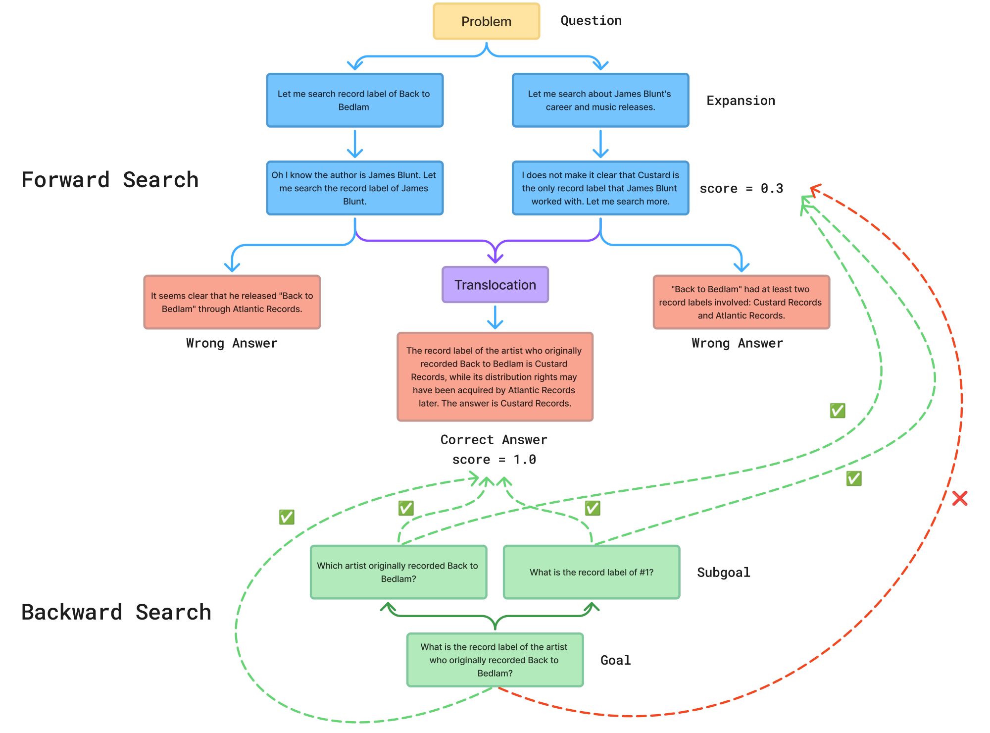
We illustrate the BES search process on a multi-hop question answering example from the MuSiQue dataset. The question is: "What is the record label of the artist who originally recorded Back to Bedlam?" The correct answer is Custard Records. Figure 5 shows the full search trace.

Backward search.

The backward search decomposes the original question into two sub-goals: (1) "Which artist originally recorded Back to Bedlam?" and (2) "What is the record label of #1?". Each sub-goal is equipped with a local verifier based on embedding similarity (Appendix D.2). This decomposition allows the search to track partial progress: a candidate that correctly identifies the artist (James Blunt) but retrieves the wrong label still receives a non-zero score, providing a useful signal for parent selection.

Forward search: expansion.

The search begins with two expansion branches from the root. The left branch searches for the record label of "Back to Bedlam" directly and concludes that the album was released through Atlantic Records, which is incorrect. The right branch takes a broader approach, searching for James Blunt's career and music releases, and discovers that both Custard Records and Atlantic Records were involved. However, it also fails to produce the correct final answer, arriving at a wrong conclusion.

Forward search: translocation.

At this point, the backward search scores both branches. The right branch receives a score of 0.3, indicating partial progress: it has identified relevant information about Custard Records but has not resolved the question correctly. The key moment occurs when the translocation operator replaces the reasoning step in the left branch (which concluded Atlantic Records) with the more nuanced reasoning step from the right branch (which noted both Custard Records and Atlantic Records). The resulting candidate inherits the left branch's identification of James Blunt as the artist and the right branch's awareness of the Custard Records connection. This recombined trajectory correctly concludes that the original record label is Custard Records, achieving a score of 1.0.

This example highlights two core advantages of BES. First, the backward search provides dense intermediate feedback: even though both initial branches produce wrong final answers, the sub-goal scores distinguish the branch that has made more relevant progress (score 0.3), enabling informed parent selection. Second, the translocation operator constructs a correct trajectory by transplanting a single useful reasoning step from one branch into another. Neither branch alone would have reached the correct answer through further expansion, but their combination via translocation succeeds. This illustrates how evolution operators can discover solutions beyond what any single policy rollout can produce.

F. Prompts for Open Problem Solving Tasks

This appendix lists the prompts used by BES on the open-problem benchmarks. The backward-search decomposition prompt (one per benchmark) elicits a JSON array of verifiable sub-goals from a goal-tree leaf, while the four evolution-operation prompts ($\textsc{diff}$, $\textsc{diff_ablate}$, $\textsc{full}$, $\textsc{cross}$) drive forward-search mutations. All prompts use Python str.format-style placeholders such as code_content, performance_metrics, previous_attempts.

F.1 Backward Search: Goal Tree Decomposition

The decomposition prompt is benchmark-specific. We list here the prompts used for Circle Packing (Square); the prompts for Circle Packing (Rectangle) and Heilbronn (Convex) follow the same structure.

```python
Decompose a circle-packing goal into smaller verifiable subgoals.

### G. Problem
Pack n=26 non-overlapping circles in [0,1]^2 to achieve sum_of_radii > 2.636 (STRICTLY EXCEED best-known).
Every candidate already satisfies validity (in-square, non-overlap, r>=0). Do NOT use those as subgoals.

### H. Elite reference layouts (top $n_e$ lites from current archive — these define the search frontier)
Look ACROSS all of them to identify:
(a) structural properties EVERY elite has -> strong reference-kind subgoals
(b) properties where elites still VARY -> indicates room for improvement, target with aspirational subgoals
(c) properties NO elite has yet but a hypothetical sum_r > best solution would have -> aspirational

elite_blocks

### I. Parent goal to decompose
goal_desc

### J. Two kinds of subgoals (BOTH required)
Produce 3-4 subgoals, MIXING the two kinds below:

A. kind="reference" (1-2 subgoals): structural properties that EVERY elite above already
   has and that naive layouts demonstrably LACK (naive grid ~ 2.4 or concentric ring ~ 2.2).
   MUST be True on every elite AND False on a uniform-radii ring/grid. Generic properties
   that any symmetric layout has (e.g. "geometric center near (0.5,0.5)", "mirror symmetry")
   are BAD — naive rings satisfy them too. Good shapes: "max radius >= some_value", "at
   least K circles with r >= some_value", "at least one pair of tangent circles with
   combined radius > some_value". Pick the threshold so EVERY elite passes.

B. kind="aspirational" (2-3 subgoals): concrete structural ideas for HOW to push sum_r
   further. These typically evaluate FALSE on most or all elites — that is the point: they
   describe what an exceed-target solution would have but the current elites still lack.
   Each must ALSO be False on naive layouts (uniform grid ~ 2.4 or ring of 26 equal circles
   ~ 2.2); otherwise a naive layout trivially passes despite a poor sum_r. Good shapes:
   - the largest circle is strictly larger than the max max_radius across elites
     (naive baselines: grid r~0.083, ring r~0.12);
   - more circles above some "large" radius cutoff than any elite achieves;
   - tighter local packing: many pairs with center-distance < $r_i + r_j +$ epsilon (tangent clusters);
   - a structural motif (hexagonal core, nested ring, dense corner clusters) requiring large radii.
   AVOID pure symmetry/centroid predicates — naive baselines satisfy them trivially.
   Set thresholds slightly beyond what the best elite exhibits — a layout that matches the
   elites still FAILS, but a layout that exceeds them can pass.

### K. Rules (both kinds)
- A strict sub-property of the parent — never a rephrasing of the parent itself.
- Pick subgoals from DIFFERENT categories: radius distribution, boundary usage, spatial
  coverage, symmetry, local geometry. Don't write variants of one idea.

### L. verify_code: return a DENSE score in [0,1], not just bool
verify_code should evaluate to a float in [0,1] representing partial credit — NOT a bool.
Use the form min(1.0, <actual> / <target>) so that progress toward the goal earns credit.
A bool is accepted (True->1.0, False->0.0) but wastes gradient; prefer dense.

CRITICAL FORMAT REQUIREMENT — single Python expression only:
  verify_code is evaluated via Python's eval(). It MUST be a single expression
  (no semicolons, no multi-line x=...; y=...; result chains, no def/for/if
  statements, no newline-separated assignments). If you need intermediate values,
  inline them or use a one-shot generator/comprehension.

### M. Output
Each subgoal:
- kind: "reference" or "aspirational".
- description: short sentence; for aspirational, briefly say WHY it pushes.
- verify_code: Python expression returning float in [0,1] (or bool). Uses centers ((26,2)),
  radii ((26,)), n=26, sum_r=float(radii.sum()), np. Must run without error.
- expected_result: typical value across the elite reference layouts (1.0 if every elite
  meets it; a fraction < 1.0 if elites only partially meet it).

Output ONLY a JSON array:

```json
[
  "kind": "reference",    "description": "...", "verify_code": "...", "expected_result": "...",
  "kind": "aspirational", "description": "...", "verify_code": "...", "expected_result": "..."
]
```

```

M.1 Forward Evolution Operations

M.1.1 Combination

```

## Current program

> **Section Summary**: The section introduces an existing program whose code is displayed as the starting point for improvement efforts. It emphasizes that any revised version must accept the same inputs and generate the same outputs while offering a more efficient internal design. Performance data for the original program is also provided to highlight areas where gains might be achieved.


Here is the current program we are trying to improve:

```{language}
code_content
```

Here are the performance metrics of the program:

performance_metrics{text_feedback_section}

## Task: trick combination

> **Section Summary**: The section describes a structured process for improving a base program by selectively borrowing one standout mechanism from each of several inspiration programs. For every candidate trick the method first checks whether it is compatible with the existing code and targets a distinct weakness; only non-conflicting mechanisms are retained. A new program is then assembled by grafting the chosen tricks onto the original skeleton, with an accompanying description that records each source and explains why the additions are expected to work together without redundancy.


Below you will see SEVERAL inspiration programs. For EACH inspiration:

1. Identify the single most distinctive trick / mechanism it uses (a particular
  initialization, a refinement step, a numerical formulation, a heuristic, ...).
2. Decide whether that trick is compatible with the current program and is likely
  additive (i.e. attacks a different failure mode than what the current program
  already handles).

Then produce a NEW full program that is the current program PLUS the compatible
tricks from the inspirations stitched in. Be explicit in the <DESCRIPTION> about
which trick came from which inspiration and why you expect them to compose
without redundancy. Drop tricks that conflict.

IMPORTANT: This is a combination, not a free rewrite. The skeleton should follow
the current program; the inspirations only contribute identifiable plug-in tricks.

Key directions to explore:

1. The optimal arrangement may involve heterogeneous or variable-sized elements
2. Strong solutions often use hybrid global-local patterns
3. The optimization routine is critical - use models with carefully tuned parameters
4. Use scipy optimize, LP, or SLSQP to optimize variables given candidate structures

```

M.1.2 Deletion

```python
## Current program

> **Section Summary**: The section introduces an existing program whose code is displayed as the starting point for improvement efforts. It emphasizes that any revised version must accept the same inputs and generate the same outputs while offering a more efficient internal design. Performance data for the original program is also provided to highlight areas where gains might be achieved.


Here is the current program. The evolution loop has been stuck on iterations of approaches similar to this one — incremental tweaks have not been moving the score:

```{language}
code_content
```

Performance metrics of the current program:

performance_metrics{text_feedback_section}

previous_attempts

## Task

> **Section Summary**: The task directs the creation of a new program by crossing over two existing code scripts, merging their strongest elements to raise performance while preserving identical inputs and outputs. It emphasizes exploring variable or heterogeneous structures, hybrid global-local patterns, and a carefully tuned optimization step that draws on tools such as scipy.optimize, linear programming, or SLSQP. The goal is framed as an iterative “translocation” exercise intended to yield a complete, improved implementation.


The current implementation has plateaued. Iterating on it further is unlikely to help. Instead:

1. Identify components of the current code that look unreasonable or that may be holding the search inside a local optimum (heuristics that don't pay off, design choices the search keeps committing to, dead branches, parameter sweeps that add little).
2. DELETE those components.
3. Rewrite the program from a fundamentally new perspective: pick an algorithm class, data structure, or strategy that the current program does NOT use, and commit fully to it.

Do not iterate on the current implementation. Do not stitch new code onto the old skeleton. Commit fully to a different approach.

A fundamental change replaces the solution representation (e.g., closed-form <-> free coordinates <-> discrete) or the search paradigm (e.g., gradient <-> sampling <-> enumeration). Swapping the optimizer, picking a sibling parametric family, or adding numerical guards are NOT fundamental changes — they leave the search trapped.

For example, the following are structurally orthogonal algorithm classes — two attempts in the same class are minor variants of each other no matter how the surface code differs:

- Closed-form analytical construction (orbit of a finite symmetry group, vertices of a known polytope, regular polygon, root-system points)
- Low-discrepancy / quasi-random sampling on a fixed domain (Halton, Sobol, Hammersley, sunflower spiral, Fibonacci lattice)
- Lattice / grid enumeration (G x G square grid, hexagonal lattice, crystallographic packing — search over subsets/labels)
- Continuous local optimization on free decision variables (gradient on a smoothed objective, SLSQP / Nelder-Mead / coordinate ascent on the raw objective)
- Population-based global search (CMA-ES, Differential Evolution, Genetic Algorithm — many parallel candidates with selection)
- Discrete combinatorial search over a finite candidate set (simulated annealing on subset selection, branch-and-bound, ILP, beam search over partial states)
- Constructive online insertion (farthest-first / k-center, max-min greedy adding one element at a time, beam search building a configuration step by step)
- Physics / relaxation methods (Lloyd / centroidal Voronoi tessellation, repulsive force fields, gradient flow with hard-margin barriers, simulated cooling on continuous coordinates)
- Algebraic / number-theoretic structure (lattice orbits of a Coxeter group, points related by a Mobius / projective map, modular-arithmetic constructions)

The list is illustrative, not exhaustive — feel free to commit to any class outside the previous attempts, including ones not above.

In the <DESCRIPTION>: name the OLD strategy in one sentence, the NEW strategy you committed to in one sentence, what you removed, and why a clean swap (not incremental tweaks) is the right move now — what local optimum the old strategy is stuck in and how the new one structurally avoids it.

Key directions to explore:

1. The optimal arrangement may involve heterogeneous or variable-sized elements
2. Strong solutions often use hybrid global-local patterns
3. The optimization routine is critical - use models with carefully tuned parameters
4. Use scipy optimize, LP, or SLSQP to optimize variables given candidate structures

```

M.1.3 Crossover

```

## Current program

> **Section Summary**: The section introduces an existing program whose code is displayed as the starting point for improvement efforts. It emphasizes that any revised version must accept the same inputs and generate the same outputs while offering a more efficient internal design. Performance data for the original program is also provided to highlight areas where gains might be achieved.


Here is the current program we are trying to improve (you will need to propose a new program with the same inputs and outputs as the original program, but with improved internal implementation):

```{language}
code_content
```

Here are the performance metrics of the program:

performance_metrics{text_feedback_section}

## Task

> **Section Summary**: The task directs the creation of a new program by crossing over two existing code scripts, merging their strongest elements to raise performance while preserving identical inputs and outputs. It emphasizes exploring variable or heterogeneous structures, hybrid global-local patterns, and a carefully tuned optimization step that draws on tools such as scipy.optimize, linear programming, or SLSQP. The goal is framed as an iterative “translocation” exercise intended to yield a complete, improved implementation.


Perform a cross-over between the code script above and the one below. Aim to combine the best parts of both code implementations that improves the score.

Provide the complete new program code.

IMPORTANT: Make sure your rewritten program maintains the same inputs and outputs as the original program, but with improved internal implementation.

Key directions to explore:

1. The optimal arrangement may involve heterogeneous or variable-sized elements
2. Strong solutions often use hybrid global-local patterns
3. The optimization routine is critical - use models with carefully tuned parameters
4. Use scipy optimize, LP, or SLSQP to optimize variables given candidate structures

```

M.1.4 Translocation

```

## Current program (the "near" parent — keep its skeleton)

```{language}
code_content
```

Performance metrics: performance_metrics{text_feedback_section}

## Task: trick translocation from a distant relative

> **Section Summary**: The task requires selecting one specific useful technique, such as a particular initialization method, constraint-handling step, or optimization heuristic, from a structurally different "donor" program. Only that single element is transplanted into the current program, with minimal adaptations to make it fit while leaving everything else unchanged. The accompanying description must justify the choice and explain why this targeted graft is preferable to broader recombination of ideas from the donor.


Below you will see ONE inspiration program drawn from the archive (a "distant
relative" — likely structurally different from the current program). Your job:

1. Read it and pick the ONE trick that is most likely to help the current
  program — a specific initialization, refinement step, constraint formulation,
  numerical detail, or heuristic. Be concrete; name it.
2. Transplant ONLY that trick into the current program. Keep the rest of the
  current program intact. Do NOT also fold in other ideas from the donor and
  do NOT broadly rewrite the recipient.
3. Adapt naming / signatures so the transplant compiles, but do not refactor
  surrounding code beyond what the transplant strictly requires.

Argue in the <DESCRIPTION>: which trick, why this one, and why grafting it onto
the current skeleton is more promising than full crossover.

Key directions to explore:

1. The optimal arrangement may involve heterogeneous or variable-sized elements
2. Strong solutions often use hybrid global-local patterns
3. The optimization routine is critical - use models with carefully tuned parameters
4. Use scipy optimize, LP, or SLSQP to optimize variables given candidate structures

```

N. Identified Programs for Open Problem Solving Tasks

This appendix summarizes, for each open-problem benchmark, the structure of the best program discovered by BES.

N.1 Circle Packing (Square)

The best program for the $n{=}26$ unit-square instance is a hybrid global optimiser. It maintains both circle centres and radii as decision variables and alternates among four ingredients: (i) a $K$-nearest-neighbour radii projection that produces a feasible packing in closed form; (ii) an active-set LP cutting-plane routine that solves for the maximum feasible radii under the current contact graph, with stateful slack counters and an annealed tightness $\tau$; (iii) a two-tier simulated-annealing search over centre perturbations with adaptive LP lock-ins and an annealed move mix; and (iv) periodic SLSQP micro-bursts on a focused subset of circles for local contact tightening. Search is launched from a portfolio of deterministic seeds, including hexagonal rows, edge rings, corner-weighted arrangements, and spokes-plus-concentric-pentagon interiors, each with controlled anisotropic jitter and short feasibility probing.

N.2 Circle Packing (Rectangle)

The best program for the $n{=}21$ rectangle-of-perimeter- $4$ instance is a deterministic multi-start constructor with a two-stage refinement. It first enumerates a dense grid of aspect ratios and a small set of jitter scales, generating candidate layouts from several heterogeneous hex-like row patterns. Each candidate is feasibility-clamped, and only the top- $K$ seeds (ranked by sum of radii, tie-broken by the minimal pairwise slack) advance to optimisation. Each surviving seed is then refined by a two-stage SLSQP: stage 1 fixes the aspect ratio with tighter bounds, and stage 2 releases the aspect ratio so all variables (centres, radii, and aspect) are co-optimised under a shrink-only feasibility projection.

N.3 Heilbronn (Convex)

The best program for the $n{=}13$ convex-hull instance commits to a $C_3$-symmetric parameterisation: one centre point and four concentric $3$-orbits (each an equilateral triangle of $3$ points at $120^{\circ}$ spacing), giving $1{+}4{\times}3=13$ points and only $8$ free parameters (four radii via a softplus-ordered map, four phases reduced modulo $2\pi/3$). Optimisation is a Coordinate Pattern Search with three custom ingredients: (i) $K$-guided weighted co-participation, where the top- $K$ smallest triangles vote on which ring to perturb next; (ii) a symmetric finite-difference $\delta v / \delta r$ sensitivity per ring with adaptive $\epsilon$ and a per-sweep cache; and (iii) per-ring adaptive step sizes with mild growth on acceptance and targeted shrink after repeated failures. The objective is the exact minimum over all $\binom{13}{3}=286$ triangles, with hull area normalised by Andrew's monotone chain plus the shoelace formula. Search is launched from a deterministic multi-seed pool with a short pre-refinement sweep before CPS.

O. Potential Limitations and Broader Impacts

Potential Limitations. We acknowledge the following limitations of the paper:

(1) BES requires an objective reward signal to guide the search. It has not been tested on subjective evaluation tasks where such signals are difficult to obtain, such as academic writing.

(2) The backward search relies on the policy's ability to decompose problems into meaningful sub-goals. For very weak models, this decomposition capability is limited.

(3) Due to resource constraints, our post-training experiments use relatively small models up to 8B parameters.

Broader Impacts. Our work proposes a general-purpose search framework for improving the quality of LLM and agent outputs. On the positive side, BES can help models achieve stronger reasoning performance, potentially reducing the need for larger models and their associated computational and environmental costs. The backward search component also improves interpretability by explicitly decomposing problems into verifiable sub-goals, making the search process more transparent. However, more effective search methods could also  enable stronger performance on tasks that could be misused.

References

Section Summary: This section compiles a numbered list of academic citations and sources referenced throughout the document. Most entries are recent papers and preprints on artificial intelligence, large language models, reasoning techniques, reinforcement learning, and related methods for improving problem-solving in AI systems. A smaller number of older references address foundational topics in genetics and statistics.

[1] Jason Wei et al. (2022). Chain of Thought Prompting Elicits Reasoning in Large Language Models. In Advances in Neural Information Processing Systems. https://openreview.net/forum?id=_VjQlMeSB_J.

[2] Zhenting Qi et al. (2025). Mutual Reasoning Makes Smaller LLMs Stronger Problem-Solver. In The Thirteenth International Conference on Learning Representations. https://openreview.net/forum?id=6aHUmotXaw.

[3] Guo et al. (2025). DeepSeek-R1 incentivizes reasoning in LLMs through reinforcement learning. Nature. 645(8081). pp. 633–638. doi:10.1038/s41586-025-09422-z. http://dx.doi.org/10.1038/s41586-025-09422-z.

[4] Alexander Novikov et al. (2025). AlphaEvolve: A coding agent for scientific and algorithmic discovery. https://arxiv.org/abs/2506.13131. arXiv:2506.13131.

[5] Hubert et al. (2026). Olympiad-level formal mathematical reasoning with reinforcement learning. Nature. 651(8106). pp. 607-613. doi:10.1038/s41586-025-09833-y. https://doi.org/10.1038/s41586-025-09833-y.

[6] Li et al. (2022). Competition-level code generation with AlphaCode. Science. 378(6624). pp. 1092–1097. doi:10.1126/science.abq1158. http://dx.doi.org/10.1126/science.abq1158.

[7] Mert Yuksekgonul et al. (2026). Learning to Discover at Test Time. https://arxiv.org/abs/2601.16175. arXiv:2601.16175.

[8] Xinyu Guan et al. (2025). rStar-Math: Small LLMs Can Master Math Reasoning with Self-Evolved Deep Thinking. In Forty-second International Conference on Machine Learning. https://openreview.net/forum?id=5zwF1GizFa.

[9] Elliot Glazer et al. (2025). FrontierMath: A Benchmark for Evaluating Advanced Mathematical Reasoning in AI. https://arxiv.org/abs/2411.04872. arXiv:2411.04872.

[10] Yang Yue et al. (2026). Does Reinforcement Learning Really Incentivize Reasoning Capacity in LLMs Beyond the Base Model?. In The Thirty-ninth Annual Conference on Neural Information Processing Systems. https://openreview.net/forum?id=4OsgYD7em5.

[11] Eric Zelikman et al. (2022). STaR: Bootstrapping Reasoning With Reasoning. In Advances in Neural Information Processing Systems. https://openreview.net/forum?id=_3ELRdg2sgI.

[12] Weizhe Yuan et al. (2024). Self-Rewarding Language Models. In Forty-first International Conference on Machine Learning. https://openreview.net/forum?id=0NphYCmgua.

[13] Eric Zelikman et al. (2024). Self-Taught Optimizer (STOP): Recursively Self-Improving Code Generation. In First Conference on Language Modeling. https://openreview.net/forum?id=46Zgqo4QIU.

[14] Yangzhen Wu et al. (2025). Inference Scaling Laws: An Empirical Analysis of Compute-Optimal Inference for LLM Problem-Solving. In The Thirteenth International Conference on Learning Representations. https://openreview.net/forum?id=VNckp7JEHn.

[15] Robert Tjarko Lange et al. (2025). ShinkaEvolve: Towards Open-Ended And Sample-Efficient Program Evolution. https://arxiv.org/abs/2509.19349. arXiv:2509.19349.

[16] Qiying Yu et al. (2025). DAPO: An Open-Source LLM Reinforcement Learning System at Scale. https://arxiv.org/abs/2503.14476. arXiv:2503.14476.

[17] Levente Kocsis and Csaba Szepesvari (2006). Bandit Based Monte-Carlo Planning. In European Conference on Machine Learning. https://api.semanticscholar.org/CorpusID:15184765.

[18] Yuxiang Ji et al. (2026). Tree Search for LLM Agent Reinforcement Learning. In The Fourteenth International Conference on Learning Representations. https://openreview.net/forum?id=ZpQwAFhU13.

[19] Shunyu Yao et al. (2023). Tree of Thoughts: Deliberate Problem Solving with Large Language Models. In Thirty-seventh Conference on Neural Information Processing Systems. https://openreview.net/forum?id=5Xc1ecxO1h.

[20] Bradley Brown et al. (2024). Large Language Monkeys: Scaling Inference Compute with Repeated Sampling. https://arxiv.org/abs/2407.21787. arXiv:2407.21787.

[21] Fisher, Ronald Aylmer (1999). The genetical theory of natural selection: a complete variorum edition. Oxford University Press.

[22] Muller, Hermann Joseph (1932). Some genetic aspects of sex. The American Naturalist. 66(703). pp. 118–138.

[23] Fahim Tajwar et al. (2026). Maximum Likelihood Reinforcement Learning. https://arxiv.org/abs/2602.02710. arXiv:2602.02710.

[24] Asankhaya Sharma (2025). OpenEvolve: an open-source evolutionary coding agent. https://github.com/algorithmicsuperintelligence/openevolve.

[25] Lakshya A Agrawal et al. (2026). GEPA: Reflective Prompt Evolution Can Outperform Reinforcement Learning. In The Fourteenth International Conference on Learning Representations. https://openreview.net/forum?id=RQm2KQTM5r.

[26] Chulin Xie et al. (2024). Large Language Interpolators Can Learn Logical Reasoning: A Study on Knights and Knaves Puzzles. In The 4th Workshop on Mathematical Reasoning and AI at NeurIPS'24. https://openreview.net/forum?id=mxX8WdPCx9.

[27] Gemma Team et al. (2025). Gemma 3 Technical Report. https://arxiv.org/abs/2503.19786. arXiv:2503.19786.

[28] Trivedi et al. (2022). MuSiQue: Multihop Questions via Single-hop Question Composition. Transactions of the Association for Computational Linguistics. 10. pp. 539–554. doi:10.1162/tacl_a_00475. https://aclanthology.org/2022.tacl-1.31/.

[29] Aaron Grattafiori et al. (2024). The Llama 3 Herd of Models. https://arxiv.org/abs/2407.21783. arXiv:2407.21783.

[30] Liu et al. (2026). SkyDiscover: A Flexible Framework for AI-Driven Scientific and Algorithmic Discovery. https://skydiscover-ai.github.io/blog.html.

[31] Audrey Huang et al. (2025). Self-Improvement in Language Models: The Sharpening Mechanism. In The Thirteenth International Conference on Learning Representations. https://openreview.net/forum?id=WJaUkwci9o.

[32] Kadlčík, Marek and Štefánik, Michal (2024). Self-training Language Models for Arithmetic Reasoning. In Findings of the Association for Computational Linguistics: EMNLP 2024. pp. 12378–12386. doi:10.18653/v1/2024.findings-emnlp.721. https://aclanthology.org/2024.findings-emnlp.721/.

[33] Aman Madaan et al. (2023). Self-Refine: Iterative Refinement with Self-Feedback. In Thirty-seventh Conference on Neural Information Processing Systems. https://openreview.net/forum?id=S37hOerQLB.

[34] Noah Shinn et al. (2023). Reflexion: language agents with verbal reinforcement learning. In Thirty-seventh Conference on Neural Information Processing Systems. https://openreview.net/forum?id=vAElhFcKW6.

[35] Guanzhi Wang et al. (2024). Voyager: An Open-Ended Embodied Agent with Large Language Models. Transactions on Machine Learning Research. https://openreview.net/forum?id=ehfRiF0R3a.

[36] Haorui Wang et al. (2025). Efficient Evolutionary Search Over Chemical Space with Large Language Models. In The Thirteenth International Conference on Learning Representations. https://openreview.net/forum?id=awWiNvQwf3.

[37] Romera-Paredes et al. (2024). Mathematical discoveries from program search with large language models. Nature. 625(7995). pp. 468–475.

[38] Hou et al. (2025). TreeRL: LLM Reinforcement Learning with On-Policy Tree Search. In Proceedings of the 63rd Annual Meeting of the Association for Computational Linguistics (Volume 1: Long Papers). pp. 12355–12369. doi:10.18653/v1/2025.acl-long.604. https://aclanthology.org/2025.acl-long.604/.

[39] Dan Zhang et al. (2024). ReST-MCTS*: LLM Self-Training via Process Reward Guided Tree Search. In The Thirty-eighth Annual Conference on Neural Information Processing Systems. https://openreview.net/forum?id=8rcFOqEud5.

[40] Yuxi Xie et al. (2024). Monte Carlo Tree Search Boosts Reasoning via Iterative Preference Learning. In The First Workshop on System-2 Reasoning at Scale, NeurIPS'24. https://openreview.net/forum?id=s004OmYP2P.

[41] Besta et al. (2024). Graph of Thoughts: Solving Elaborate Problems with Large Language Models. Proceedings of the AAAI Conference on Artificial Intelligence. 38(16). pp. 17682–17690. doi:10.1609/aaai.v38i16.29720. http://dx.doi.org/10.1609/aaai.v38i16.29720.

[42] Hao et al. (2023). Reasoning with Language Model is Planning with World Model. In Proceedings of the 2023 Conference on Empirical Methods in Natural Language Processing. pp. 8154–8173. doi:10.18653/v1/2023.emnlp-main.507. https://aclanthology.org/2023.emnlp-main.507/.

[43] Kou Misaki et al. (2025). Wider or Deeper? Scaling LLM Inference-Time Compute with Adaptive Branching Tree Search. In ICLR 2025 Workshop on Foundation Models in the Wild. https://openreview.net/forum?id=3HF6yogDEm.

[44] Yiping Wang et al. (2025). ThetaEvolve: Test-time Learning on Open Problems. https://arxiv.org/abs/2511.23473. arXiv:2511.23473.

[45] Julien Pourcel et al. (2026). Self-Improving Language Models for Evolutionary Program Synthesis: A Case Study on ARC-AGI. https://arxiv.org/abs/2507.14172. arXiv:2507.14172.

[46] Hart et al. (1968). A Formal Basis for the Heuristic Determination of Minimum Cost Paths. IEEE Transactions on Systems Science and Cybernetics. 4(2). pp. 100-107. doi:10.1109/TSSC.1968.300136.

[47] Eugene L. Lawler and D. E. Wood (1966). Branch-and-Bound Methods: A Survey. Oper. Res.. 14. pp. 699-719. https://api.semanticscholar.org/CorpusID:36099120.

[48] Holland, John H. (1992). Adaptation in Natural and Artificial Systems: An Introductory Analysis with Applications to Biology, Control, and Artificial Intelligence. The MIT Press. doi:10.7551/mitpress/1090.001.0001. https://doi.org/10.7551/mitpress/1090.001.0001.

[49] Banzhaf et al. (2000). Genetic programming. IEEE Intelligent Systems and their Applications. 15(3). pp. 74-84. doi:10.1109/5254.846288.

[50] Storn, Rainer and Price, Kenneth (1997). Differential Evolution – A Simple and Efficient Heuristic for Global Optimization over Continuous Spaces. J. of Global Optimization. 11(4). pp. 341–359. doi:10.1023/A:1008202821328. https://doi.org/10.1023/A:1008202821328.