
Functional Gradient Descent with Adaptive Representations
Daniel Csillag1^{1}1, Rodrigo Schuller2^{2}2 Pedro Dall'Antonia1^{1}1, Leonidas Guibas3^{3}3, Luiz Velho2^{2}2, Tiago Novello2,3^{2,3}2,3
1^{1}1FGV EMAp 2^{2}2IMPA 3^{3}3Stanford University
Abstract
Functional optimization problems are typically solved by optimizing the parameters of a fixed representation, such as a neural network, resulting in highly nonconvex losses that complicate both training and theoretical analysis. An interesting alternative is functional gradient descent (FGD), that is, gradient descent directly in function space, which benefits from strong convergence results and admits a clean theory. However, FGD is difficult to implement in practice because functional gradients are infinite-dimensional, and thus cannot be fully computed nor stored in memory. Existing implementations therefore rely on fixed approximations, which introduce approximation error. We propose a new, theoretically-grounded FGD algorithm that adapts the representation of the functional gradients over the course of optimization. By explicitly incorporating this approximation into the analysis, we establish convergence to a stationary point (for smooth losses) and to a global minimizer (under smoothness + a Polyak-Łojasiewicz-type condition) regardless of our approximations. To the best of our knowledge, this is the first implementable FGD method with such guarantees in a general setting. We demonstrate the effectiveness of our method on regression, numerical solution of PDEs, and modern computer vision. Across settings, our method consistently outperforms both FGD with fixed approximations and neural network baselines in efficiency and accuracy.
1. Introduction
Functional optimization problems are core to many areas, including machine learning, statistics, signal processing, scientific computing, and more. In these settings, the objective is to optimize a function over a function space to minimize some loss (e.g., mean squared error or cross-entropy).
To solve such problems, it is common to represent the target function as a neural network and optimize the loss over the network's weights through gradient descent. While flexible, this introduces some challenges: (i) the resulting optimization problem is highly nonconvex, making training costly; (ii) the representation is typically fixed a priori, limiting its ability to adapt during optimization; and (iii) the nonconvex nature of the parametrized loss significantly complicates theoretical analyses of convergence and training dynamics.
We instead consider gradient descent directly in function space — functional gradient descent (FGD) — whose dynamics are generally simpler than their parameterized counterparts and admit strong convergence guarantees. Formally, consider the optimization problem
where H\mathcal{H}H is a Hilbert space of functions (e.g., L2L^2L2, Sobolev spaces, or an RKHS1). Under suitable differentiability conditions, the (non-parametric) loss admits a well-defined functional gradient ∇L(h)∈H\nabla L(h) \in \mathcal{H}∇L(h)∈H, allowing us to write the FGD updates
1.
Reproducing Kernel Hilbert Space
From a theoretical point of view, FGD is well known to benefit from good convergence guarantees (cf. e.g. ([1, 2])). However, it is nontrivial to implement in practice. Since the functional gradients reside in the infinite-dimensional space H\mathcal{H}H, they generally cannot be computed exactly nor stored in memory. As a result, to actually implement FGD we must approximate the gradients ∇L(ft)\nabla L(f_t)∇L(ft) via some finite-dimensional representation. Yet using a fixed representation introduces approximation error, preventing convergence to a global minimizer.
In this paper, we propose a new theoretically-grounded functional gradient descent algorithm that adapts the representation of the functional gradients over the course of optimization. We show that by adaptively refining the gradient approximations so as to ensure a certain bound on a relative error condition, we guarantee sufficient descent and thus proper convergence. To the best of our knowledge,
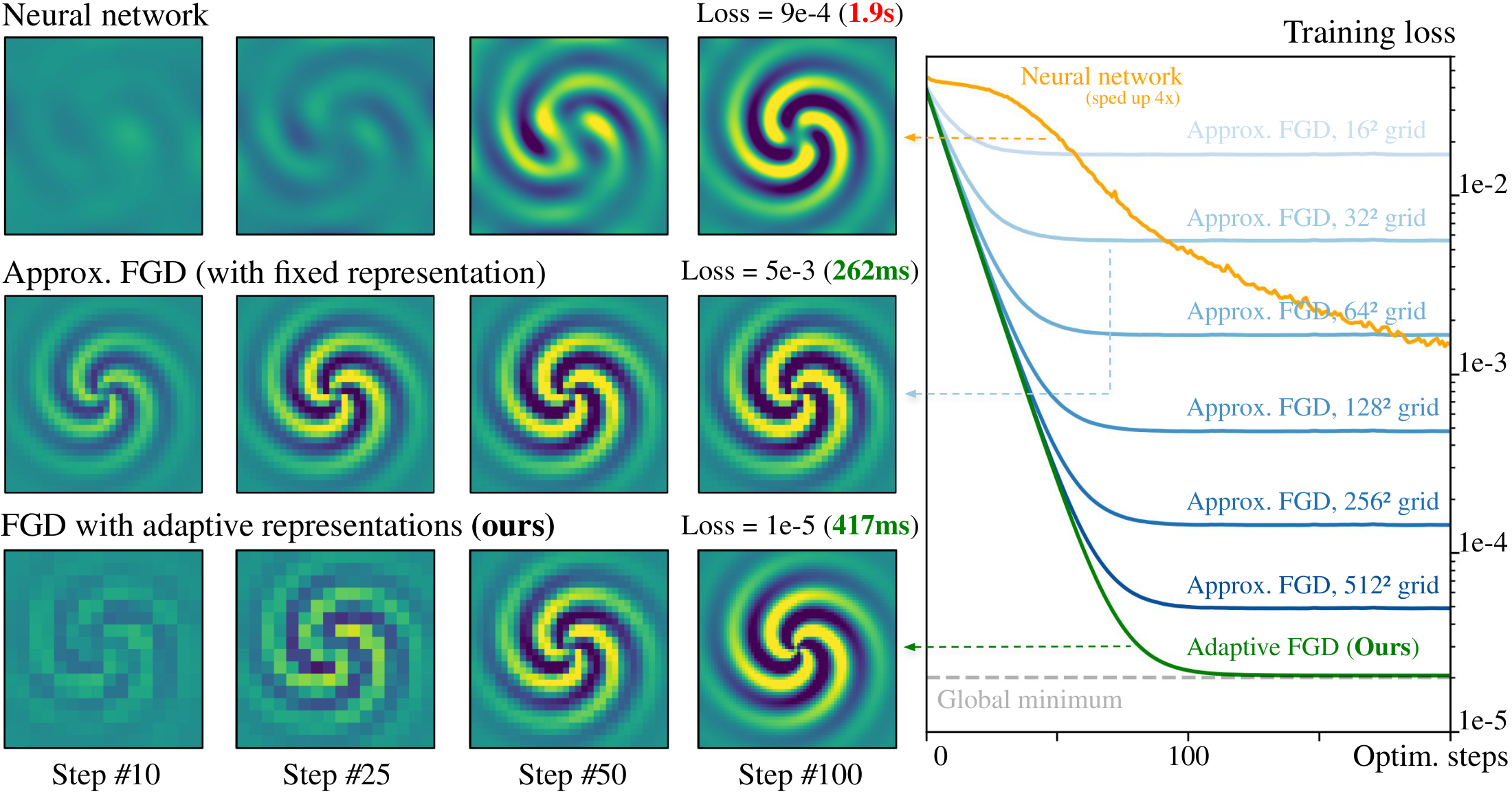
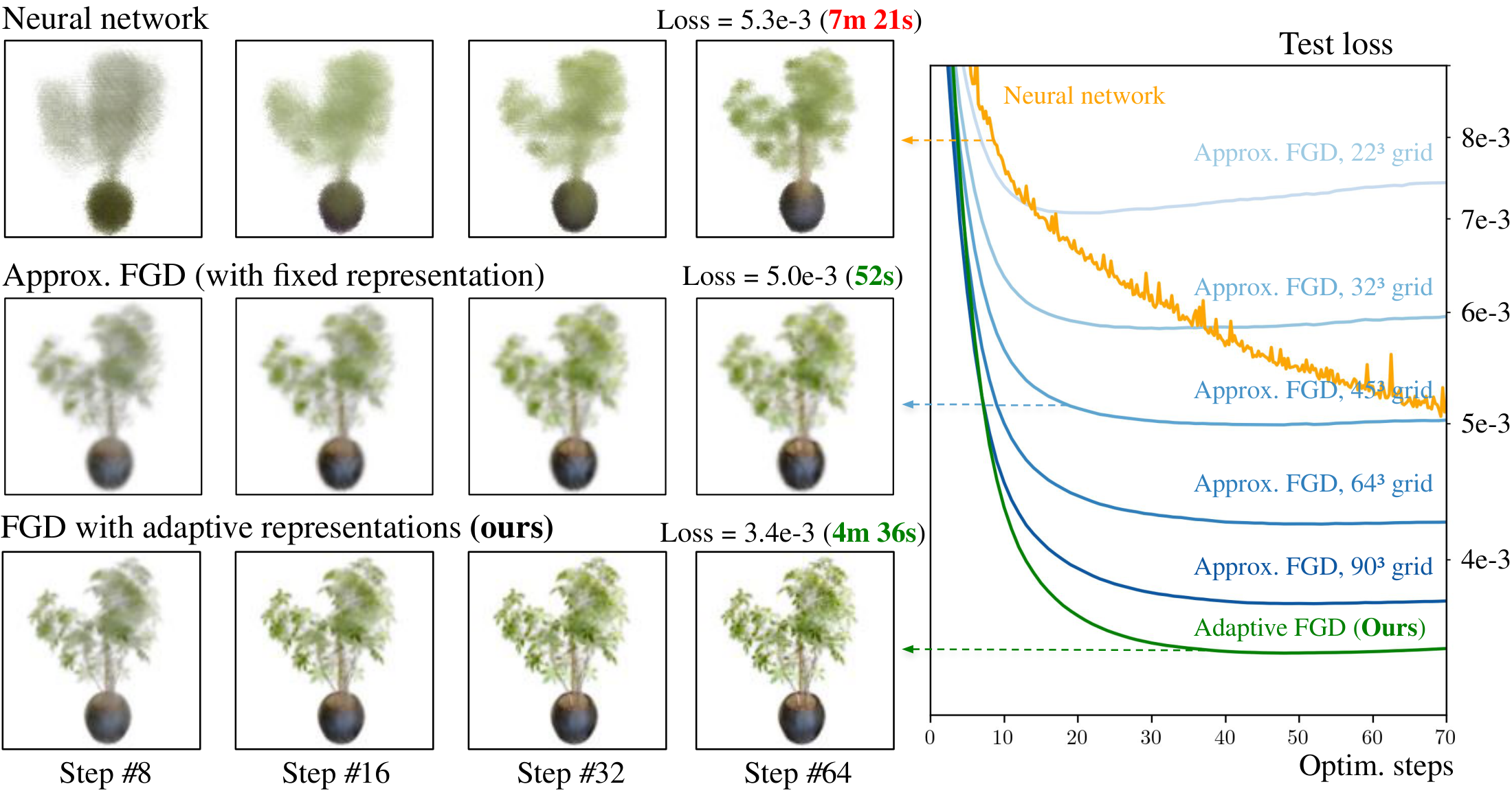
ours is the first implementable FGD method that guarantees convergence to a global minimizer. The resulting procedure strictly outperforms functional gradient descent with any fixed representation, and simultaneously outperforms neural networks in both training speed and quality; see Figure 1.
Our main contributions are:
- We establish sufficient conditions for the proper convergence of approximate FGD. Notably, our analysis covers the general setting where true gradients lie in a Hilbert space but are approximated within a broader Banach space, enabling important functional optimization tasks. We prove that maintaining a specific relative error bound guarantees convergence to a stationary point for smooth losses, and to a global minimizer under an additional Polyak-Łojasiewicz-type condition.
- We develop novel gradient approximation strategies that provably satisfy our derived relative error condition, using only computable quantities. This yields the first fully implementable FGD algorithms that retain strict, end-to-end convergence guarantees.
- We evaluate our method on three representative tasks across regression in an RKHS, numerical PDE solvers, and modern computer vision. On all settings, our adaptive approach consistently surpasses FGD using any fixed representation, while substantially outperforming neural network baselines in both training efficiency and solution quality.
Related work FGD is well-established as a theoretical procedure; see, e.g. ([2]) for an overview of the convergence theory for exact FGD. In specific cases, exact FGD is actually feasible to implement; for example, in the specific case of standard regression losses over an RKHS, the gradients are finite-dimensional and can therefore be exactly represented. This is akin to the classic representer theorems for kernel regression ([3, 4]). However, such approaches rely on specific finite-sample structures, do not generalize beyond simple regression settings, and typically scale poorly with sample size. Alternatively, several works approximate functional gradients ([5, 6, 7, 8, 9]), but introduce irreducible approximation error and often do not incorporate this approximation into their theoretical analysis. Our work addresses this by (i) providing a general theory for approximate FGD, and (ii) identifying sufficient conditions that ensure convergence to proper minimizers sans approximation error.
Our work is also related to first-order optimization with inexact gradients ([10, 11, 12]), but differs in that we operate in the infinite-dimensional setting, where many previous methods break down. In particular, most approximation schemes (e.g. ([13, 2, 14])) do not extend to infinite dimensions. Additionally, we consider a more general setting in which gradients lie in a Hilbert space but are approximated in a broader Banach space, beyond the scope of existing theory.
2. Background: function spaces and functional gradients
We briefly recall function spaces and differentiability in infinite dimensions. A Hilbert space H\mathcal{H}H is a complete inner product space, endowed with ⟨⋅,⋅⟩H\langle \cdot, \cdot \rangle_\mathcal{H}⟨⋅,⋅⟩H and induced norm ∥h∥H=⟨h,h⟩H\lVert h \rVert_\mathcal{H} = \sqrt{\langle h, h \rangle_\mathcal{H}}∥h∥H=⟨h,h⟩H. Similarly, a Banach space B\mathcal{B}B is a complete normed space with norm ∥⋅∥B\lVert \cdot \rVert_\mathcal{B}∥⋅∥B, but generally does not admit an inner product. Every Banach space B\mathcal{B}B admits a dual space B∗\mathcal{B}^*B∗, consisting of continuous linear functionals on B\mathcal{B}B, which is itself a Banach space under the dual norm ∥u∥B∗=sup∥b∥B≤1∣u(b)∣\lVert u \rVert_{\mathcal{B}^*} = \sup_{\lVert b \rVert_\mathcal{B} \leq 1} \lvert u(b) \rvert∥u∥B∗=sup∥b∥B≤1∣u(b)∣.
Let L:H→RL : \mathcal{H} \to \mathbb{R}L:H→R be a functional. The directional derivative of LLL at fff in the direction f⃗\vec{f}f is defined as
If DL\mathrm{D} LDL exists for all f,f⃗f, \vec{f}f,f and is linear over f⃗\vec{f}f, LLL is Gâteaux differentiable; additionally, if DL\mathrm{D} LDL is continuous in fff, then LLL is Fréchet differentiable.2
2.
This is equivalent to the usual definition of Fréchet derivatives as bounded linear operators, ([15]).
When LLL is Fréchet differentiable over a Hilbert space H\mathcal{H}H, for every f∈Hf \in \mathcal{H}f∈H the map DL(f;⋅)\mathrm{D} L(f; \cdot)DL(f;⋅) (i.e., the functional f⃗↦DL(f;f⃗)\vec{f} \mapsto \mathrm{D} L(f; \vec{f})f↦DL(f;f)) is a continuous linear functional. Therefore, by the Riesz representation theorem, there exists a unique element ∇L(f)∈H\nabla L(f) \in \mathcal{H}∇L(f)∈H such that
This element ∇L(f)\nabla L(f)∇L(f) is the functional gradient, defining the gradient operator ∇L:H→H\nabla L : \mathcal{H} \to \mathcal{H}∇L:H→H. When H=Rd\mathcal{H} = \mathbb{R}^dH=Rd with the standard inner product, this recovers the usual notion of gradients.
Finally, while Hilbert spaces provide a convenient structure for defining gradients, they can impose significant constraints on their elements. For instance, the empirical MSE functional
is not well-defined on L2(R)L^2(\mathbb{R})L2(R) (space of square-integrable functions), since functions in L2(R)L^2(\mathbb{R})L2(R) cannot be evaluated on a set of measure zero. In contrast, it is well-defined in RKHSs, which enforce additional regularity but are more restrictive than L2(R)L^2(\mathbb{R})L2(R).
Nevertheless, these issues arise due to the requirement of a proper inner product. Once we move from Hilbert to Banach spaces, we can use flexible function spaces such as L∞L^\inftyL∞ or the space of continuous functions, without caveats.
3. Method
Let H\mathcal{H}H be a Hilbert space contained in a Banach space B\mathcal{B}B, and recall the optimization problem 1
where L:H→RL : \mathcal{H} \to \mathbb{R}L:H→R is taken to be a Fréchet differentiable functional on H\mathcal{H}H. Since H\mathcal{H}H is a Hilbert space, the derivative of LLL admits a gradient operator ∇L:H→H\nabla L : \mathcal{H} \to \mathcal{H}∇L:H→H (cf. Section 2). An ideal functional gradient descent (FGD) scheme would, therefore, perform the steps
which remain strictly within H\mathcal{H}H and whose convergence follows by the standard proofs of convergence of FGD. However, since this is intractable to implement, we instead replace the gradient by an approximate gradient gtg_tgt, yielding updates
where gt∈Bg_t \in \mathcal{B}gt∈B (and thus the iterates ftf_tft also reside in B\mathcal{B}B). We will show that as long as gtg_tgt approximates ∇L(ft)\nabla L(f_t)∇L(ft) reasonably well (in a sense we will make precise), we still guarantee descent and proper convergence. Subsequently, we shall study strategies to guarantee that the required approximation conditions hold in practice by adaptively refining the gradient representations.
3.1 Convergence
In order to analyze the convergence of the updates in Equation 4, we must introduce some assumptions. First, note that loss and gradient operator are defined over the Hilbert space H\mathcal{H}H, but our updates will reside in the larger Banach space B\mathcal{B}B; therefore, in order to keep things well-defined, our first assumption is that both the loss LLL and the gradient operator ∇L\nabla L∇L have extensions from H\mathcal{H}H onto B\mathcal{B}B:
Assumption 1: Extension
There exists a Fréchet differentiable functional L‾:B→R\overline{L} : \mathcal{B} \to \mathbb{R}L:B→R and an operator ∇L‾:B→B\overline{\nabla L} : \mathcal{B} \to \mathcal{B}∇L:B→B such that, for any f∈Hf \in \mathcal{H}f∈H,
For convenience, from here on we will slightly abuse notation and "shadow" LLL and ∇L\nabla L∇L by their extended counterparts; i.e., for some f∈Bf \in \mathcal{B}f∈B we shall write L(f)L(f)L(f) instead of L‾(f)\overline{L}(f)L(f), and similarly we shall write ∇L(f)\nabla L(f)∇L(f) instead of ∇L‾(f)\overline{\nabla L}(f)∇L(f).
We will additionally rely on the standard assumptions used for the analysis of gradient descent, albeit over the larger Banach space B\mathcal{B}B rather than the usual Hilbert H\mathcal{H}H. In particular, we will assume that the loss is KKK-smooth:
Assumption 2: -smoothness
For any f,f′∈Bf, f' \in \mathcal{B}f,f′∈B, it holds that
Note that we write the KKK-smoothness bound in terms of the directional derivative DL\mathrm{D} LDL rather than an inner product with the gradient, as the Banach space does not generally have an inner product.
We will also require two additional assumptions, which serve to connect the gradients between the Banach space B\mathcal{B}B and the Hilbert space H\mathcal{H}H:
Assumption 3: descends in
There exists some constant α>0\alpha>0α>0 such that, for all f∈Bf \in \mathcal{B}f∈B,
Assumption 4: Gradient compatibility
There exists a constant β>0\beta > 0β>0 such that, for every f∈Bf \in \mathcal{B}f∈B,
When B=H\mathcal{B} = \mathcal{H}B=H both of these assumptions are immediately satisfied with α=β=1\alpha = \beta = 1α=β=1: DL(f;∇L(f))=⟨∇L(f),∇L(f)⟩H=∥∇L(f)∥H2\mathrm{D} L(f; \nabla L(f)) = \langle \nabla L(f), \nabla L(f) \rangle_\mathcal{H} = \lVert \nabla L(f) \rVert_\mathcal{H}^2DL(f;∇L(f))=⟨∇L(f),∇L(f)⟩H=∥∇L(f)∥H2, and ∥DL(f;⋅)∥B∗=∥∇L(f)∥B\lVert \mathrm{D} L(f; \cdot) \rVert_{\mathcal{B}^*} = \lVert \nabla L(f) \rVert_{\mathcal{B}}∥DL(f;⋅)∥B∗=∥∇L(f)∥B. But these assumptions are more general, and satisfied in some important cases where H≠B\mathcal{H} \neq \mathcal{B}H=B (cf. Section 4.1). Intuitively, Assumption 3 asserts that the direction given by the extended gradient ∇L(f)\nabla L(f)∇L(f) is guaranteed to be a direction of sufficient descent per the geometry of B\mathcal{B}B. Assumption 4, on the other hand, establishes a sort of local equivalence of norms over the gradients (but not over the whole space).
With these in hand, we can analyze a single step of our method Equation (4) to establish a sufficient descent lemma. The following result follows from the KKK-smoothness inequality (Assumption 2), along with our Assumption 3 and Assumption 4 and the use of triangular inequalities:
Lemma 5: Sufficient descent lemma
Let ft,ft+1f_t, f_{t+1}ft,ft+1 be as in Equation 4. Suppose LLL and ∇L\nabla L∇L admit extensions satisfying KKK-smoothness, gradient compatibility and that H\mathcal{H}H descends in B\mathcal{B}B (Assumption 1-Assumption 4). Then, for any learning rate η>0\eta > 0η>0 and step ttt with RelErr(gt,∇L(ft))≤1/2\mathrm{RelErr}(g_t, \nabla L(f_t)) \leq 1/2RelErr(gt,∇L(ft))≤1/2,
where
Note that this bound is tight, in the sense that when H=B\mathcal{H} = \mathcal{B}H=B, gt=∇L(ft)g_t = \nabla L(f_t)gt=∇L(ft), and η=1/K\eta = 1/Kη=1/K, we recover the usual descent lemma L(ft−ηgt)≤L(ft)−η2∥∇L(ft)∥B2L(f_t - \eta g_t) \leq L(f_t) - \frac{\eta}{2} \lVert \nabla L(f_t) \rVert_\mathcal{B}^2L(ft−ηgt)≤L(ft)−2η∥∇L(ft)∥B2 (cf. e.g. ([16])).
As long as the term within the brackets is strictly positive, we guarantee that a step of approximate functional gradient descent decreases the loss in a manner proportional to the current gradient value. By telescoping and rearranging we obtain:
Proposition 6: Convergence to a stationary point
Under the setting of Lemma 5, furthermore assume that the loss is lower bounded by L⋆L^\starL⋆, and that the relative error is uniformly bounded by a constant ϵ<min{1/2,α/(α+β)}\epsilon < \min \{ 1/2, \alpha/(\alpha+\beta) \}ϵ<min{1/2,α/(α+β)} throughout iterations:
Then, for any learning rate η≤2(α−(α+β)ϵ)/K(2ϵ+1)\eta \leq 2 (\alpha - (\alpha + \beta) \epsilon) / K ( 2\epsilon + 1 )η≤2(α−(α+β)ϵ)/K(2ϵ+1),
where r>0r>0r>0 is a constant defined in the proof.
Under additional structural assumptions we are able to furthermore establish convergence to the proper global minimizer. For our purposes, we will work under a Polyak-Łojasiewicz-type assumption, which serves as a generalization of strong convexity:
Assumption 7: Polyak-Łojasiewicz condition on over
The extended Fréchet-differentiable functional L:B→RL : \mathcal{B} \to \mathbb{R}L:B→R is μ\muμ-Polyak-Łojasiewicz if, for any f∈Bf \in \mathcal{B}f∈B,
It then holds:
Proposition 8: Global convergence
Under the conditions of Proposition 6, further assume that LLL is μ\muμ-Polyak-Łojasiewicz (Assumption 7). Then, for any learning rate η<2(α−(α+β)ϵ)/K(2ϵ+1)\eta < 2 (\alpha - (\alpha + \beta) \epsilon) / K (2\epsilon + 1)η<2(α−(α+β)ϵ)/K(2ϵ+1), performing TTT iterations of approximate functional gradient descent guarantees that
3.2 Adaptive representations of functional gradients
In the previous section we have established that as long as we can ensure an upper bound on the relative error, we guarantee proper convergence. In this section, we now consider how exactly we can approximate the functional gradient so as to guarantee this will be the case.
Recall that our ultimate objective is to find some gradient approximation ggg that ensures that the relative error is bounded by some fixed ϵ\epsilonϵ:
Note that while the denominator can generally be computed exactly (as it is the norm of our own approximation), the approximation error in the numerator can still be tricky. However, it is often possible to compute a (reasonably tight) upper bound U(g,∇L(f))U(g, \nabla L(f))U(g,∇L(f)) on ∥g−∇L(f)∥B\lVert g - \nabla L(f) \rVert_\mathcal{B}∥g−∇L(f)∥B, in the sense that
With such an upper bound in hand, we can guarantee:
Lemma 9
Given some f∈Bf \in \mathcal{B}f∈B and desired tolerance ϵ>0\epsilon>0ϵ>0, let U(⋅,⋅)U(\cdot, \cdot)U(⋅,⋅) be an upper bound on the approximation error (as in Equation 6), and let (g1,g2,…)(g_1, g_2, \ldots)(g1,g2,…) be a sequence of gradient approximations in B\mathcal{B}B such that U(gn,∇L(f))→0U(g_n, \nabla L(f)) \to 0U(gn,∇L(f))→0. Then there exists some nnn such that
The result in Lemma 9 is quite general. Importantly, it suggests a concrete algorithm: at each FGD step we design a sequence of representations, and loop over this sequence; at each iterate, approximate the gradient using the current representation and compute the upper bound on the approximation error. As soon as Equation 7 is satisfied (which must happen at some point, as per Lemma 9), we use the current approximation. Algorithm 1 gives the overall procedure.
Connecting with our previous convergence theory, we obtain:
Theorem 1
Let ftf_tft be the iterates produced throughout Algorithm 1, with ϵ∈(0,1)\epsilon \in (0, 1)ϵ∈(0,1). Then:
- (i) Relative error bound: For all iterations t=1,…,Tt = 1, \ldots, Tt=1,…,T,
- (ii) Convergence to a stationary point: Under the conditions of Proposition 6,
where r>0r>0r>0 is a constant defined in the proof; and
- (iii) Convergence to a global minimizer: Under the conditions of Proposition 8,
4. Experiments
In this section we empirically assess our method on three representative functional optimization tasks: regression in an RKHS, solution of partial differential equations and inverse rendering. Throughout, we focus on comparing our method against (i) neural networks (with appropriate engineering), and (ii) FGD with fixed representations.
All experiments were run on a desktop with an Intel Core i9-14900KF CPU and NVIDIA GeForce RTX 4090 GPU, with 128GB of RAM and 24GB of VRAM, respectively. That said, the experiments are relatively cheap and should run on weaker hardware. Code to reproduce our results can be found at https://github.com/dccsillag/experiments-adaptive-fgd. In all experiments the learning rates were tuned to obtain the best possible performance of each method.
4.1 Regression in an RKHS
In this section we consider the optimization problem
where HK\mathcal{H}_KHK is an RKHS with kernel KKK. Here, ℓ\ellℓ denotes a pointwise loss such as the mean squared error (ℓ(y^,y)=12(y^−y)2\ell(\hat{y}, y) = \frac{1}{2} (\hat{y} - y)^2ℓ(y^,y)=21(y^−y)2) or binary cross-entropy (ℓ(y^,y)=−ylogy^−(1−y)log(1−y^)\ell(\hat{y}, y) = -y \log \hat{y} - (1-y) \log (1-\hat{y})ℓ(y^,y)=−ylogy^−(1−y)log(1−y^)). Such regression problems are commonplace in statistical inference procedures, including conditional independence testing ([17]), asymptotic statistics ([18]), and more.
The loss LREGL_\mathrm{REG}LREG admits simple functional gradients, is KKK-smooth and Polyak-Łojasiewicz:
Proposition 10
The functional LREG:HK→RL_\mathrm{REG} : \mathcal{H}_K \to \mathbb{R}LREG:HK→R has gradients given by
where ℓ′\ell'ℓ′ denotes the derivative of ℓ\ellℓ with respect to its first argument. Moreover, if ℓ\ellℓ is strongly-convex in its first argument, then LREGL_\mathrm{REG}LREG is Polyak-Łojasiewicz, and if ℓ\ellℓ is KKK-smooth then so is LREGL_\mathrm{REG}LREG.
As mentioned in Section 2, the space HK\mathcal{H}_KHK is generally quite constrained. For this reason, in this experiment we opt to approximate the gradients in the larger Banach space L∞L^\inftyL∞ of bounded functions, which can be checked to satisfy our gradient bridging assumptions (Assumption 3 and Assumption 4), cf. Proposition 12. For our adaptive representations we then choose a decision tree-based approximation scheme inspired by the classic CART algorithm (which reside in L∞L^\inftyL∞, but generally not in HK\mathcal{H}_KHK). By using sufficiently deep trees we are able to approximate functions arbitrarily well, allowing us to use Lemma 9 and thus ensure convergence as per Theorem 1.
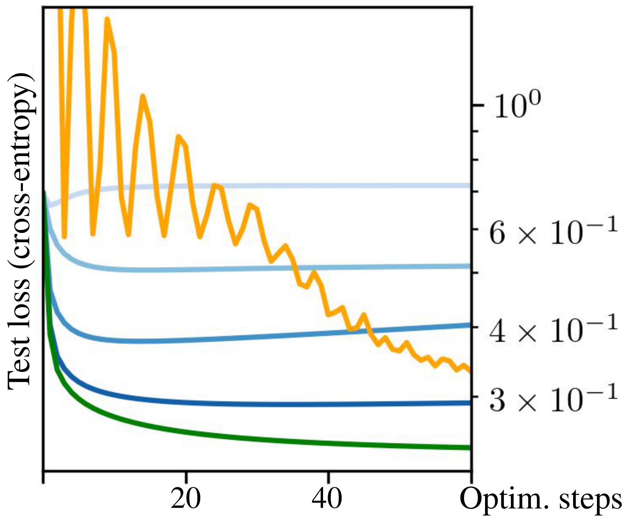
For this experiment we use the binary classification dataset of ([19]) for the detection of non-coding RNA sequences. We consider two losses ℓ\ellℓ: mean squared error and binary cross entropy. Figure 2 shows the results of our experiment. We find that our method consistently outperforms a standard MLP neural network as well as FGD with any fixed representation, adapting as necessary to the target function and guaranteeing convergence to the global optimum while achieving a better test loss.
4.2 Solving the wave equation
This section shows how our method can be applied to physics-informed machine learning tasks ([20, 21]). As an example, consider the wave equation for f:R×R2→Rf: \mathbb{R}\times \mathbb{R}^2\to \mathbb{R}f:R×R2→R,
which models wave propagation phenomena such as sound, mechanical vibrations, and electromagnetic waves ([22, 23, 24, 25]). Although solutions exist under broad conditions on the initial data hhh, explicit closed-form solutions are generally unavailable in realistic settings, requiring numerical approximation methods.
We can formulate solving Equation 9 as minimizing the following loss functional
which vanishes if and only if fff solves Equation 9. The functional is defined over the Sobolev space H=H2(R3)\mathcal{H} = H^2(\mathbb{R}^3)H=H2(R3) so that the second-order derivatives are well-defined.
Computing functional gradients in Sobolev spaces is generally challenging ([7]). However, the Fourier transform of the gradient admits a closed-form expression:
Proposition 11
Let ω:=τ2−c2(ξ2+ζ2)\omega := \tau^2 - c^2(\xi^2+\zeta^2)ω:=τ2−c2(ξ2+ζ2). The Fourier transform of the gradient of LPDEL_\mathrm{PDE}LPDE is
We therefore approximate gradients using adaptive uniform grids in frequency space. Each grid defines a piecewise-constant approximation of the Fourier transform f^\widehat{f}f, while the corresponding function fff is recovered through the inverse Fourier transform. Moreover, the Fourier representation of the H2(R3)H^2(\mathbb{R}^3)H2(R3) norm yields a straightforward upper bound on the gradient approximation error.
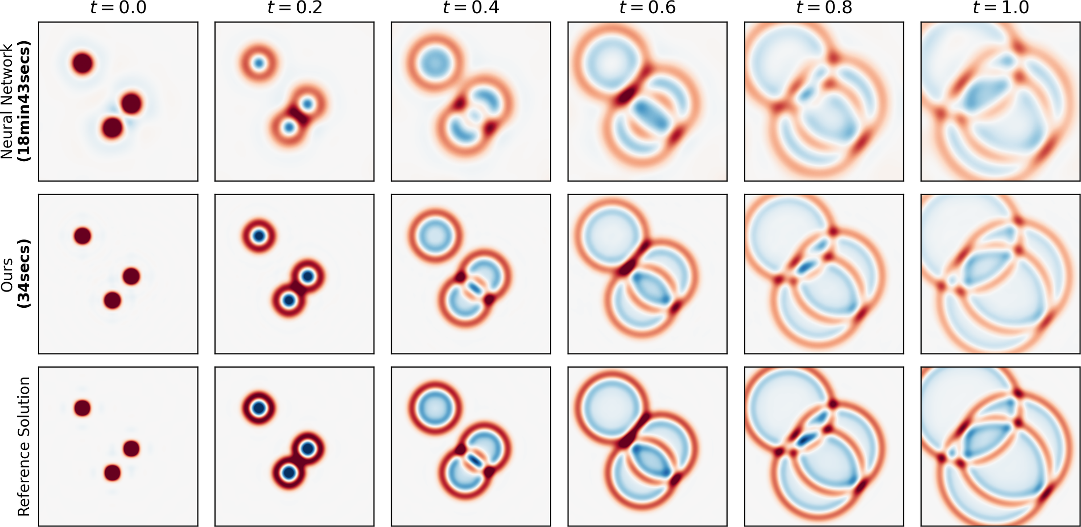
Figure 3 shows the results. Our adaptive method consistently outperforms FGD with fixed representations, which quickly plateaus due to approximation error. It also surpasses the neural network baseline while reducing wall-clock training time by nearly two orders of magnitude.
4.3 Learning radiance fields
We next consider the inverse rendering task of reconstructing a 3D scene from posed images ([26]). This can be framed as a functional optimization problem: given images with known camera parameters, the goal is to learn the scene as a density field and a view-dependent color field,
Given a camera ray γ:[tnear,tfar]→R3\gamma : [t_\mathrm{near},t_\mathrm{far}]\to \mathbb{R}^3γ:[tnear,tfar]→R3 with viewing direction γω\gamma_\omegaγω, where tneart_\mathrm{near}tnear and tfart_\mathrm{far}tfar denote integration bounds, we can render the scene via the volumetric rendering equation ([27]) with distributional antialiasing ([28]), yielding the antialiased rendering operator R~σ,c(γ)\widetilde{R}_{\sigma,c}(\gamma)Rσ,c(γ), which is differentiable w.r.t. σ\sigmaσ and ccc. Then, given a set of pixels (Yi,j)i=1,j=1n,P(Y_{i,j})_{i=1,j=1}^{n,P}(Yi,j)i=1,j=1n,P and corresponding rays (γi,j)i=1,j=1n,P(\gamma_{i,j})_{i=1,j=1}^{n,P}(γi,j)i=1,j=1n,P originating from the respective cameras i=1,…,ni = 1, \ldots, ni=1,…,n, our goal is to optimize the loss
which is well-defined for σ∈L2(Ω)\sigma \in L^2(\Omega)σ∈L2(Ω) and c∈L2(Ω→HS)c \in L^2(\Omega \to \mathcal{H}^{\mathbb{S}})c∈L2(Ω→HS), where Ω\OmegaΩ is a compact subset of R3\mathbb{R}^3R3 and HS\mathcal{H}^\mathbb{S}HS is an RKHS with domain over the unit sphere S2\mathbb{S}^2S2. This loss directly measures image reconstruction error and is the standard supervision signal for radiance-field optimization (cf. e.g. ([26, 29])). It is highly nonconvex; nonetheless, it has functional gradients known in closed form, cf. Appendix A.1.4, which we efficiently approximate by the means of uniform 3D grids with spherical harmonics for the color view-dependence.
We evaluate on the Ficus scene from the NeRF-Synthetic dataset ([26]), using the same camera poses and train/test split for all methods. All methods optimize the photometric loss in Equation 10; we compare adaptive FGD with an Adam-trained neural network baseline and fixed-grid FGD variants. As shown in Figure 4, adaptive FGD achieves the lowest test loss and sharpest reconstructions by starting coarse and refining only when needed, whereas fixed-grid FGD plateaus at a resolution-dependent error floor and the neural baseline converges much more slowly.
Acknowledgments
We'd like to thank Google for partially funding this work. We also acknowledge partial funding from CNPq and FAPERJ.
Appendix
A. Proofs
Proof of Lemma 5: Let us derive the bound in the lemma. By KKK-smoothness, we have that
Writing gt=∇L(ft)−(∇L(ft)−gt)=:∇L(ft)−etg_t = \nabla L(f_t) - (\nabla L(f_t) - g_t) =: \nabla L(f_t) - e_tgt=∇L(ft)−(∇L(ft)−gt)=:∇L(ft)−et, it follows:3
to simplify the expression, let us assume that ∥∇L(ft)−gt∥B/∥∇L(ft)∥B=∥et∥B/∥∇L(ft)∥B≤1{\lVert \nabla L(f_t) - g_t \rVert_\mathcal{B}}/{\lVert \nabla L(f_t) \rVert_\mathcal{B}} = {\lVert e_t \rVert_\mathcal{B}}/{\lVert \nabla L(f_t) \rVert_\mathcal{B}} \leq 1∥∇L(ft)−gt∥B/∥∇L(ft)∥B=∥et∥B/∥∇L(ft)∥B≤1. This allows us to use the fact that x2≤xx^2 \leq xx2≤x for ∣x∣≤1\lvert x \rvert \leq 1∣x∣≤1 to write
3.
Throughout, we follow the convention that and for all .
As long as the expression within the parentheses is positive, we ensure descent. However, the relative error ∥∇L(ft)−gt∥B/∥∇L(ft)∥B{\lVert \nabla L(f_t) - g_t \rVert_\mathcal{B}}/{\lVert \nabla L(f_t) \rVert_\mathcal{B}}∥∇L(ft)−gt∥B/∥∇L(ft)∥B is a bit tricky to manage in practice since the denominator involves the ∥∇L(ft)∥B\lVert \nabla L(f_t) \rVert_\mathcal{B}∥∇L(ft)∥B, which can be hard to tightly lower bound. Fortunately, we can replace it with ∥gt∥B\lVert g_t \rVert_\mathcal{B}∥gt∥B, which can be generally be computed exactly; indeed, by the reverse triangle inequality,4
rearranging, we obtain that
and thus
where
finally, to guarantee that ∥gt−∇L(ft)∥B/∥∇L(ft)∥B≤1{\lVert g_t - \nabla L(f_t) \rVert_\mathcal{B}}/{\lVert \nabla L(f_t) \rVert_\mathcal{B}} \leq 1∥gt−∇L(ft)∥B/∥∇L(ft)∥B≤1 as required, it suffices to require RelErr(gt,∇L(ft))≤1/2\mathrm{RelErr}(g_t, \nabla L(f_t)) \leq 1/2RelErr(gt,∇L(ft))≤1/2, as 12/(1−12)=1\frac{1}{2} / (1 - \frac{1}{2}) = 121/(1−21)=1. Putting it all together, we obtain the desired bound.
4.
; as an immediate consequence, .
Proof of Proposition 6: It follows:
where the first inequality holds by Lemma 5, and the second by the assumption that RelErr(gt,∇L(ft))≤ϵ\mathrm{RelErr}(g_t, \nabla L(f_t)) \leq \epsilonRelErr(gt,∇L(ft))≤ϵ for all t=1,…,Tt = 1, \ldots, Tt=1,…,T.
Rearranging and scaling by 1/T1/T1/T on both sides, we get
dividing by r=[α−Kη2−(β+32Kη)ϵ1−ϵ]r = \left[ \alpha - \frac{K \eta}{2} - \left( \beta + \frac{3}{2} K \eta \right) \frac{\epsilon}{1-\epsilon} \right]r=[α−2Kη−(β+23Kη)1−ϵϵ] on both sides yields the desired bound; to show that r>0r>0r>0, simply note that
which is positive thanks to the upper bound on ϵ\epsilonϵ.
Proof of Proposition 8: We have that
where the first inequality holds by Lemma 5, the second by the assumption that RelErr(gt,∇L(ft))≤ϵ\mathrm{RelErr}(g_t, \nabla L(f_t)) \leq \epsilonRelErr(gt,∇L(ft))≤ϵ for all t=1,…,Tt = 1, \ldots, Tt=1,…,T, and the third by the Polyak-Łojasiewicz assumption. Rearranging:
chaining these over t=0,…,T−1t = 0, \ldots, T-1t=0,…,T−1 yields
Proof of Lemma 9: First, note that by the sandwich theorem,
Then, by continuity,
and so
The result then follows by the definition of the limit of a sequence: for any ϵ>0\epsilon > 0ϵ>0, there exists some nnn such that the bound is satisfied for all n′≥nn' \geq nn′≥n – which, in particular, must hold for nnn itself.
Proof of Theorem 1: Let us start by establishing claim (i). For Algorithm 1 to perform a gradient descent step, we must have that
i.e., that
and since ∥gt−∇L(ft)∥B≤Ut\lVert g_t - \nabla L(f_t) \rVert_\mathcal{B} \leq U_t∥gt−∇L(ft)∥B≤Ut, we have that
where the last inequality follows by the fact that ϵ∈(0,1)\epsilon \in (0, 1)ϵ∈(0,1). Additionally, by Lemma 9, the while loop is guaranteed to terminate, allowing the algorithm to proceed.
Claims (ii) and (iii) then follow immediately by applying Proposition 6 and Proposition 8.
A.1 Computation of Functional Derivatives for the Experiments
A.1.1 Function fitting (Figure 1)
We consider here the loss LFIT:L2([0,1]2)→RL_\mathrm{FIT} : L^2([0,1]^2) \to \mathbb{R}LFIT:L2([0,1]2)→R given by
It holds:
Proposition
The functional LFIT:L2([0,1]2)→RL_\mathrm{FIT} : L^2([0,1]^2) \to \mathbb{R}LFIT:L2([0,1]2)→R has gradients given by
and is 1-Polyak-Łojasiewicz.
Proof: The directional derivative is
and so
To show that the loss is 1-Polyak-Łojasiewicz, note:
A.1.2 Regression in an RKHS (Section 4.1)
Proof of Proposition 10: The directional derivative is
and thus
To establish that the loss is Polyak-Łojasiewicz, note that the loss depends on fff only through its evaluations at the data points. Let v∈Rnv \in \mathbb{R}^nv∈Rn with vi=f(Xi)v_i = f(X_i)vi=f(Xi), and let g(v)=1n∑i=1nℓ(vi,Yi)g(v) = \frac{1}{n} \sum_{i=1}^n \ell(v_i, Y_i)g(v)=n1∑i=1nℓ(vi,Yi). Because ℓ\ellℓ is μ\muμ-strongly convex in its first argument, ggg is strongly convex with respect to the Euclidean norm with parameter μ/n\mu/nμ/n.
Letting ci=ℓ′(f(Xi),Yi)c_i = \ell'(f(X_i), Y_i)ci=ℓ′(f(Xi),Yi), the gradient is ∇g(v)=1nc\nabla g(v) = \frac{1}{n} c∇g(v)=n1c. By standard strong convexity, the suboptimality is bounded by the gradient norm:
We must now bound ∥c∥22\lVert c \rVert_2^2∥c∥22 using the L∞L^\inftyL∞ norm of the extended RKHS gradient. Recall that the continuous extension of the gradient to B=L∞\mathcal{B} = L^\inftyB=L∞ is the function:
Let K∈Rn×nK \in \mathbb{R}^{n \times n}K∈Rn×n be the empirical kernel matrix, and let gX∈Rng_X \in \mathbb{R}^ngX∈Rn be the evaluation of this gradient at the training points, so gX(i)=∇LREG(f)(Xi)g_X^{(i)} = \nabla L_\mathrm{REG}(f)(X_i)gX(i)=∇LREG(f)(Xi). In matrix form, we have gX=1nKcg_X = \frac{1}{n} K cgX=n1Kc.
Assuming the kernel matrix KKK is strictly positive definite, we can invert this relationship to get c=nK−1gXc = n K^{-1} g_Xc=nK−1gX. Bounding the Euclidean norm of ccc via the smallest eigenvalue λmin(K)>0\lambda_{\min}(K) > 0λmin(K)>0 yields:
Next, we bound the discrete Euclidean norm ∥gX∥2\lVert g_X \rVert_2∥gX∥2 by the supremum norm over the entire space. Since ∣gX(i)∣≤supx∣∇LREG(f)(x)∣=∥∇LREG(f)∥L∞\lvert g_X^{(i)} \rvert \leq \sup_x \lvert \nabla L_\mathrm{REG}(f)(x) \rvert = \lVert \nabla L_\mathrm{REG}(f) \rVert_{L^\infty}∣gX(i)∣≤supx∣∇LREG(f)(x)∣=∥∇LREG(f)∥L∞ for all iii, we have:
Substituting this back into the bound for ∥c∥2\lVert c \rVert_2∥c∥2, we get:
Finally, plugging this into our suboptimality bound yields:
Finally, to show that LREGL_\mathrm{REG}LREG is KKK-smooth: let f,f′∈L∞f, f' \in L^\inftyf,f′∈L∞. Using the definition of LREGL_\mathrm{REG}LREG and applying the KKK-smoothness of ℓ\ellℓ to each data point XiX_iXi, we have:
Next, we bound the quadratic term using the definition of the L∞L^\inftyL∞ norm. Since ∣f(Xi)−f′(Xi)∣≤supx∣f(x)−f′(x)∣=∥f−f′∥L∞\lvert f(X_i) - f'(X_i) \rvert \leq \sup_{x} \lvert f(x) - f'(x) \rvert = \lVert f - f' \rVert_{L^\infty}∣f(Xi)−f′(Xi)∣≤supx∣f(x)−f′(x)∣=∥f−f′∥L∞ for all iii, it follows that:
Substituting this back into our inequality yields:
Proposition 12
Let LREGL_\mathrm{REG}LREG be the regression functional over HK\mathcal{H}_KHK, and assume the empirical kernel matrix K∈Rn×nK \in \mathbb{R}^{n \times n}K∈Rn×n over the training data is strictly positive definite with minimum eigenvalue λmin(K)>0\lambda_{\min}(K) > 0λmin(K)>0. Furthermore, assume the kernel is bounded, such that supx,x′∣K(x,x′)∣≤κ\sup_{x, x'} \lvert K(x, x') \rvert \leq \kappasupx,x′∣K(x,x′)∣≤κ. Then, evaluating the gradients over the Banach space B=L∞\mathcal{B} = L^\inftyB=L∞, the loss LREGL_\mathrm{REG}LREG satisfies:
- (i) Gradient compatibility (Assumption 4): with constant β=nλmin−1(K)\beta = n \lambda_{\min}^{-1}(K)β=nλmin−1(K).
- (ii) H\mathcal{H}H descends in B\mathcal{B}B (Assumption 3): with constant α=λmin(K)nκ2\alpha = \frac{\lambda_{\min}(K)}{n \kappa^2}α=nκ2λmin(K).
Proof: As established previously, let ci=ℓ′(f(Xi),Yi)c_i = \ell'(f(X_i), Y_i)ci=ℓ′(f(Xi),Yi) for i=1,…,ni=1, \dots, ni=1,…,n, such that the continuous extension of the gradient to B=L∞\mathcal{B} = L^\inftyB=L∞ is ∇LREG(f)(x)=1n∑i=1nciK(Xi,x)\nabla L_\mathrm{REG}(f)(x) = \frac{1}{n} \sum_{i=1}^n c_i K(X_i, x)∇LREG(f)(x)=n1∑i=1nciK(Xi,x). The directional derivative for any f⃗∈L∞\vec{f} \in L^\inftyf∈L∞ is DLREG(f;f⃗)=1n∑i=1ncif⃗(Xi)\mathrm{D} L_\mathrm{REG}(f; \vec{f}) = \frac{1}{n} \sum_{i=1}^n c_i \vec{f}(X_i)DLREG(f;f)=n1∑i=1ncif(Xi).
For gradient compatibility, we must show that ∥DLREG(f;⋅)∥(L∞)∗≤β∥∇LREG(f)∥L∞\lVert \mathrm{D} L_\mathrm{REG}(f; \cdot) \rVert_{(L^\infty)^*} \leq \beta \lVert \nabla L_\mathrm{REG}(f) \rVert_{L^\infty}∥DLREG(f;⋅)∥(L∞)∗≤β∥∇LREG(f)∥L∞. Recall that the dual norm of the directional derivative over L∞L^\inftyL∞ is exactly the scaled L1L_1L1 norm of the coefficients:
Let gX∈Rng_X \in \mathbb{R}^ngX∈Rn be the vector of gradient evaluations at the training points, so gX(i)=∇LREG(f)(Xi)g_X^{(i)} = \nabla L_\mathrm{REG}(f)(X_i)gX(i)=∇LREG(f)(Xi). In matrix form, gX=1nKcg_X = \frac{1}{n} K cgX=n1Kc, which gives c=nK−1gXc = n K^{-1} g_Xc=nK−1gX. By the definition of the supremum norm, the maximum absolute evaluation of the gradient over the entire domain bounds the maximum absolute evaluation at the training points: ∥gX∥∞≤∥∇LREG(f)∥L∞\lVert g_X \rVert_\infty \leq \lVert \nabla L_\mathrm{REG}(f) \rVert_{L^\infty}∥gX∥∞≤∥∇LREG(f)∥L∞.
It then follows:
Substituting this into the dual norm equation and applying ∥gX∥∞≤∥∇LREG(f)∥L∞\lVert g_X \rVert_\infty \leq \lVert \nabla L_\mathrm{REG}(f) \rVert_{L^\infty}∥gX∥∞≤∥∇LREG(f)∥L∞ yields:
Thus, gradient compatibility holds with β=nλmin−1(K)\beta = n \lambda_{\min}^{-1}(K)β=nλmin−1(K).
To establish that H\mathcal{H}H descends in B\mathcal{B}B, we must show DLREG(f;∇LREG(f))≥α∥∇LREG(f)∥L∞2\mathrm{D} L_\mathrm{REG}(f; \nabla L_\mathrm{REG}(f)) \geq \alpha \lVert \nabla L_\mathrm{REG}(f) \rVert_{L^\infty}^2DLREG(f;∇LREG(f))≥α∥∇LREG(f)∥L∞2. Evaluating the directional derivative in the direction of the gradient yields:
We now require an upper bound for ∥∇LREG(f)∥L∞2\lVert \nabla L_\mathrm{REG}(f) \rVert_{L^\infty}^2∥∇LREG(f)∥L∞2 in terms of c⊤Kcc^\top K cc⊤Kc. Using the triangle inequality and the kernel bound κ\kappaκ:
Squaring both sides and applying the norm inequality ∥c∥12≤n∥c∥22\lVert c \rVert_1^2 \leq n \lVert c \rVert_2^2∥c∥12≤n∥c∥22, we have:
By the Rayleigh quotient for positive definite matrices, c⊤Kc≥λmin(K)∥c∥22c^\top K c \geq \lambda_{\min}(K) \lVert c \rVert_2^2c⊤Kc≥λmin(K)∥c∥22, meaning ∥c∥22≤λmin−1(K)c⊤Kc\lVert c \rVert_2^2 \leq \lambda_{\min}^{-1}(K) c^\top K c∥c∥22≤λmin−1(K)c⊤Kc. Substituting this gives:
Rearranging to isolate the quadratic form c⊤Kcc^\top K cc⊤Kc:
Since the left side is exactly DLREG(f;∇LREG(f))\mathrm{D} L_\mathrm{REG}(f; \nabla L_\mathrm{REG}(f))DLREG(f;∇LREG(f)), the condition is satisfied with α=λmin(K)nκ2\alpha = \frac{\lambda_{\min}(K)}{n \kappa^2}α=nκ2λmin(K).
A.1.3 Solving Partial Differential Equations (Section 4.2)
Proof of Proposition 11: The directional derivative is
Now, we have to rewrite this as an inner product on H2(R3)H^2(\mathbb{R}^3)H2(R3). Recall how the Sobolev inner product can be given in terms of the Fourier transform ([30]):
Therefore, let us rewrite the directional derivative to be of this form. To start, we will make it so that all references to fff are through its Fourier transform, each term at a time:
For the initial condition terms, we will use the fact that
It then follows:
and
Putting it all together, we obtain:
therefore, we have
A.1.4 Learning radiance fields
Our scene is represented as a pair of functions
corresponding to the density and color components, respectively; note that the color (returned in RGB) is taken to be view-dependent, while the density is view-independent.
With this functional representation of the scene, an infinitesimal ray γ:[tnear,tfar]→R3\gamma : [t_\mathrm{near}, t_\mathrm{far}] \to \mathbb{R}^3γ:[tnear,tfar]→R3 with direction γω:=γ(tfar)−γ(tnear)∥γ(tfar)−γ(tnear)∥\gamma_\omega := \frac{\gamma(t_\mathrm{far}) - \gamma(t_\mathrm{near})}{\left\lVert{\gamma(t_\mathrm{far}) - \gamma(t_\mathrm{near})}\right\rVert}γω:=∥γ(tfar)−γ(tnear)∥γ(tfar)−γ(tnear) can be rendered through
where b∈R3b \in \mathbb{R}^3b∈R3 is a fixed background color and Tσ(⋅)T_\sigma(\cdot)Tσ(⋅) is the transmittance, defined as
To render a full image from a scene, it will furthermore be useful to refer to an antialiased rendering operation. Given a position in the image plane p:=(u,v)∈R2p := (u, v) \in \mathbb{R}^2p:=(u,v)∈R2, with corresponding infinitesimal rays given by γp=γu,v\gamma_p = \gamma_{u,v}γp=γu,v, we render by convolution with an antialiasing kernel k~:R2→R\widetilde{k} : \mathbb{R}^2 \to \mathbb{R}k:R2→R as
Ideally k~\widetilde{k}k would be taken to be a sinc kernel so as to compensate for the sampling of the signal, though in practice it would be a more computable choice such as a bicubic filter. Note that this can also be seen as a continuous version of supersampling antialiasing.
With these in hand, our goal is to solve a functional optimization problem
over NNN training cameras&images, each with PPP pixels; here pi,jp_{i,j}pi,j corresponds to the position in the pixel plane, and Yi,j∈R3Y_{i,j} \in \mathbb{R}^3Yi,j∈R3 corresponds to the color of the jjj-th pixel of the iii-th image. A position in pixel plane p=(u,v)p = (u,v)p=(u,v) is mapped to the ray
where A∈R3×3A \in \mathbb{R}^{3 \times 3}A∈R3×3 is the camera transformation matrix, fff is the focal length and o∈R3o \in \mathbb{R}^3o∈R3 is the camera position.
To treat this as an optimization problem in function space, we must first consider the domain of the loss functional L(⋅,⋅)L(\cdot, \cdot)L(⋅,⋅), so as to ensure that functional gradients are well-defined. To this end, let us first assume that the 3D domain of the density and color functions is contained to a Ω⊂R3\Omega \subset \mathbb{R}^3Ω⊂R3 that is compact (i.e., bounded and closed), endowed with the Lebesgue measure over Ω\OmegaΩ. We then take the density function to reside in standard L2L^2L2 space over Ω\OmegaΩ, denoted L2(Ω→R)L^2(\Omega \to \mathbb{R})L2(Ω→R); the color function, on the other hand, has to be taken to be on a "mixture" of being L2L^2L2 in the position x∈Ω⊂R3x \in \Omega \subset \mathbb{R}^3x∈Ω⊂R3 but following a more tame RKHS structure in the direction ω∈S2\omega \in S^2ω∈S2; this can be done by writing the color in curried form
where HS\mathcal{H}^\mathbb{S}HS is a reproducing kernel Hilbert space (RKHS) of functions from the unit sphere S2S^2S2 to R\mathbb{R}R. This is necessary so as to make the loss functional LLL well-defined over a Hilbert space of functions. The RKHS HS\mathcal{H}^\mathbb{S}HS comes endowed with a reproducing kernel KHS:HS×HS→RK_{\mathcal{H}^\mathbb{S}} : \mathcal{H}^\mathbb{S} \times \mathcal{H}^\mathbb{S} \to \mathbb{R}KHS:HS×HS→R, defined by the reproducing property that ⟨h,KHS(ω,⋅)⟩=⟨h,KHS(⋅,ω)⟩=h(ω)\left\langle{ h, K_{\mathcal{H}^\mathbb{S}}(\omega, \cdot) }\right\rangle = \left\langle{ h, K_{\mathcal{H}^\mathbb{S}}(\cdot, \omega) }\right\rangle = h(\omega)⟨h,KHS(ω,⋅)⟩=⟨h,KHS(⋅,ω)⟩=h(ω) for any h∈HSh \in \mathcal{H}^\mathbb{S}h∈HS and ω∈S2\omega \in S^2ω∈S2.
Proposition 13
Suppose the antialiasing kernel k~(⋅,⋅)\widetilde{k}(\cdot, \cdot)k(⋅,⋅) has a non-empty support, and define the antialiased color differences
Then the loss functional L:L2(Ω→R)×L2(Ω→[HS]3)→RL : L^2(\Omega \to \mathbb{R}) \times L^2(\Omega \to [\mathcal{H}^\mathbb{S}]^3) \to \mathbb{R}L:L2(Ω→R)×L2(Ω→[HS]3)→R is Fréchet differentiable, with gradients given by
for constants ai:=fi21[t(x;i)∈F]/Pt(x;i)2∣detAi∣a_i := f_i^2 \mathbf{1}[t(x;i) \in F] / P t(x;i)^2 \lvert\det A_i\rvertai:=fi21[t(x;i)∈F]/Pt(x;i)2∣detAi∣.
Note that when the antialiasing kernel k~\widetilde{k}k has compact support, D~σ,c(x;i,j)\widetilde{D}_{\sigma,c}(x; i,j)Dσ,c(x;i,j) can be efficiently computed by considering just a neighborhood around the jjj-th pixel.
Proof of Proposition 13: Let us start by deriving the directional (Gâteaux) derivative. It is handy to rewrite it as a scalar derivative evaluated at zero:
It then follows by straightforward computation:
Now, the remaining derivative is as follows. For convenience, we let γ≡γu′,v′\gamma \equiv \gamma_{u',v'}γ≡γu′,v′.
Now, a slightly tricky step: in the second term, let's swap the integrals.
And now, we can turn this all into an L2L^2L2 inner product.
Plugging this back into the full directional derivative:
Now, to help transform this into an L2L^2L2 inner product, let us introduce a lemma.
Lemma
For the iii-th camera and any g:R3→Rg : \mathbb{R}^3 \to \mathbb{R}g:R3→R,
where F=[tnear,tfar]F = [t_\mathrm{near}, t_\mathrm{far}]F=[tnear,tfar], and Ai,fiA_i, f_iAi,fi are camera parameters.
Proof (of the lemma): First write γu′,v′(t)=oi+tAiqu′,v′\gamma_{u',v'}(t) = o_i + t A_i q_{u',v'}γu′,v′(t)=oi+tAiqu′,v′, for qu′,v′=(u′/fi,−v′/fi,−1)q_{u',v'} = (u'/f_i, -v'/f_i, -1)qu′,v′=(u′/fi,−v′/fi,−1); so we have the triple integral
where p(⋅;i)p(\cdot; i)p(⋅;i) is such that p(o+tAqu′,v′;i)=(u′,v′)p(o + t A q_{u',v'}; i) = (u',v')p(o+tAqu′,v′;i)=(u′,v′), and
We will do a change-of-variables with Φ\PhiΦ. Note that it is invertible and differentiable, with Jacobian matrix as follows:
Now, let D=R2×[tnear,tfar]D = \mathbb{R}^2 \times [t_\mathrm{near}, t_\mathrm{far}]D=R2×[tnear,tfar]. By integration by substitution,
and by the inverse function theorem,
So, applying the lemma, we have that
And thus, the functional gradients are given by:
and using D~σ,c(x;i,j)=∑j=1P(R~σ,c(pi,j)−Yi,j) k~(p(x;i)−pi,j)\widetilde{D}_{\sigma,c}(x; i,j) = \sum_{j=1}^P ( \widetilde{{R}}_{\sigma,c}(p_{i,j}) - Y_{i,j} ) \, \widetilde{k}(p(x;i)-p_{i,j})Dσ,c(x;i,j)=∑j=1P(Rσ,c(pi,j)−Yi,j)k(p(x;i)−pi,j) and ai=(fi21[t(x;i)∈F])/(Pt(x;i)2∣detAi∣)a_i = (f_i^2 \mathbf{1}[t(x;i) \in F])/(P t(x;i)^2 \lvert\det A_i\rvert)ai=(fi21[t(x;i)∈F])/(Pt(x;i)2∣detAi∣) we obtain
This establishes that LLL is (linearly) Gâteaux differentiable. It is also immediately seen to be Fréchet differentiable, as the gradients are continuous with relation to σ\sigmaσ and ccc.
B. Experiment details
B.1 Regression in an RKHS
For the experiments we use an RBF kernel K(x,y)=exp(−100∥x−y∥2)K(x, y) = \exp(-100 \lVert x - y \rVert^2)K(x,y)=exp(−100∥x−y∥2). We use a simple tree-based approximation scheme which naively partitions splits at the midpoints. This is mainly for ease of (efficient) implementation in JAX, and in no way fundamental to our approach. To upper bound the approximation error, we use the fact that our trees are piecewise constant over rectangular partitions of the space, and bound the sup-norm of each leaf via a Lipschitz bound on the gradient (using the fact that the RBF kernel is Lipschitz). The neural network is a standard MLP with two hidden layers of size 256; we note that modifying this doesn't change the conclusions in any significant manner.
B.2 Solving the wave equation
The neural network baseline has a Fourier feature embedding layer ([31]), which is essential for the neural network to even be capable of optimizing this loss; without this embedding, no matter how large (or small) the network or optimizer hyperparameters, it stays stuck and does not fit the solution at all. As the loss has an integral in its definition, the neural network optimizes it on batches of 4096 points uniformly sampled over the domain; lowering this batch size leads to worse results. For our method, the inverse Fourier transform can be directly computed as a sum of sincs, using the fact that a box function in frequency space corresponds to a sinc in the primary space. Finally, we bound the approximation error via a combination of a Lipschitz argument (for the interior of the frequency-space grid) and a bound on the Sobolev symbol for the content outside of the grid. For the reference solution in the figure, we solve the equation using a finite differences method with an extremely fine grid.
B.3 Learning radiance fields
We train our method on 24 160×160160 \times 160160×160 RGB images, and evaluate on 25 160×160160 \times 160160×160 RGB images of novel views on the test subset. Both Approx. FGD (all resolutions) and Adaptive FGD used identical optimization hyperparameters. They employed a learning rate of 8 for the color function ccc and 20 for the density function σ\sigmaσ, approximated the gradient by taking 8 samples per voxel and averaging them for the density, and fitting spherical harmonics coefficients through one step of Newton's method. On the other hand, the NN used Adam optimizer with learning rate of 1e−41e-41e−4 and β=(0.9,0.999)\beta = (0.9, 0.999)β=(0.9,0.999). Since the NN cannot perform full-batch gradient descent due to VRAM limitations, we used mini-batches of 80×8080\times 8080×80 rays and counted 4×244 \times 244×24 mini-batches as an optimization step (to match the full-batch updates of our method). Note that, since the NN traces one ray per pixel, 4×244 \times 244×24 mini-batches correspond exactly to the number of rays in the full training data.
References
[1] Bauschke, Heinz H. and Combettes, Patrick Louis (2017). Convex analysis and monotone operator theory in Hilbert spaces. Springer. https://hal.sorbonne-universite.fr/hal-01517477.
[2] Jorge Nocedal and Stephen J. Wright (2004). Numerical optimization. The Mathematical Gazette. 88. pp. 412 - 413. https://api.semanticscholar.org/CorpusID:189864167.
[3] George Kimeldorf and Grace Wahba (1971). Some results on Tchebycheffian spline functions. Journal of Mathematical Analysis and Applications. 33. pp. 82-95. https://api.semanticscholar.org/CorpusID:121062339.
[4] Bernhard Scholkopf et al. (2001). A Generalized Representer Theorem. In COLT/EuroCOLT. https://api.semanticscholar.org/CorpusID:9256459.
[5] Yuri Fonseca and Yuri F. Saporito (2022). Statistical Learning and Inverse Problems: An Stochastic Gradient Approach. ArXiv. abs/2209.14967. https://api.semanticscholar.org/CorpusID:252595623.
[6] C. Peixoto et al. (2024). Nonparametric Instrumental Variable Regression through Stochastic Approximate Gradients. ArXiv. abs/2402.05639. https://api.semanticscholar.org/CorpusID:267547764.
[7] C. Peixoto et al. (2025). Random Gradient-Free Optimization in Infinite Dimensional Spaces. https://api.semanticscholar.org/CorpusID:284133189.
[8] Ieva Petrulionyte et al. (2024). Functional Bilevel Optimization for Machine Learning. ArXiv. abs/2403.20233. https://api.semanticscholar.org/CorpusID:268793583.
[9] Kaheon Kim et al. (2025). Sobolev Gradient Ascent for Optimal Transport: Barycenter Optimization and Convergence Analysis. ArXiv. abs/2505.13660. https://api.semanticscholar.org/CorpusID:278769678.
[10] Olivier Devolder et al. (2013). First-order methods of smooth convex optimization with inexact oracle. Mathematical Programming. 146. pp. 37 - 75. https://api.semanticscholar.org/CorpusID:1624627.
[11] Alexandre d'Aspremont (2005). Smooth Optimization with Approximate Gradient. SIAM J. Optim.. 19. pp. 1171-1183. https://api.semanticscholar.org/CorpusID:208328.
[12] Mark W. Schmidt et al. (2011). Convergence Rates of Inexact Proximal-Gradient Methods for Convex Optimization. ArXiv. abs/1109.2415. https://api.semanticscholar.org/CorpusID:11262278.
[13] Albert S. Berahas et al. (2019). A Theoretical and Empirical Comparison of Gradient Approximations in Derivative-Free Optimization. Foundations of Computational Mathematics. 22. pp. 507 - 560. https://api.semanticscholar.org/CorpusID:146120814.
[14] Yurii Nesterov and Vladimir G. Spokoiny (2015). Random Gradient-Free Minimization of Convex Functions. Foundations of Computational Mathematics. 17. pp. 527 - 566. https://api.semanticscholar.org/CorpusID:2147817.
[15] Hemant Kumar Pathak (2018). An Introduction to Nonlinear Analysis and Fixed Point Theory. https://api.semanticscholar.org/CorpusID:126068909.
[16] Stephen J. Wright and Benjamin Recht (2022). Optimization for Data Analysis. https://api.semanticscholar.org/CorpusID:247919424.
[17] Kun Zhang et al. (2011). Kernel-based Conditional Independence Test and Application in Causal Discovery. ArXiv. abs/1202.3775. https://api.semanticscholar.org/CorpusID:18509113.
[18] van der Vaart, A. W. (1998). Asymptotic Statistics. Cambridge University Press.
[19] Fan, Rong-En and Lin, Chih-Jen (2011). LIBSVM Data: Classification, Regression, and Multi-label. https://www.csie.ntu.edu.tw/~cjlin/libsvmtools/datasets/. Accessed: 2026-05-07.
[20] Raissi et al. (2019). Physics-informed neural networks: A deep learning framework for solving forward and inverse problems involving nonlinear partial differential equations. Journal of Computational physics. 378. pp. 686–707.
[21] Bizzi et al. (2025). Neuro-Spectral Architectures for Causal Physics-Informed Networks. In Advances in Neural Information Processing Systems.
[22] Evans, Lawrence C. (2010). Partial Differential Equations. American Mathematical Society.
[23] Jackson, John David (1999). Classical Electrodynamics. Wiley.
[24] Jensen et al. (2011). Computational ocean acoustics. Springer.
[25] Marques et al. (2025). Stable adaptive training for physics-informed neural networks in acoustic wave propagation. JASA Express Letters. 5(11). pp. 112401.
[26] Mildenhall et al. (2021). Nerf: Representing scenes as neural radiance fields for view synthesis. Communications of the ACM. 65(1). pp. 99–106.
[27] Max, Nelson (1995). Optical models for direct volume rendering. IEEE Transactions on Visualization and Computer Graphics. 1(2). pp. 99–108.
[28] Cook et al. (1984). Distributed ray tracing. In Proceedings of the 11th annual conference on Computer graphics and interactive techniques. pp. 137–145.
[29] Kerbl et al. (2023). 3d gaussian splatting for real-time radiance field rendering.. ACM Trans. Graph.. 42(4). pp. 139–1.
[30] Evans, Lawrence C (2022). Partial differential equations. American mathematical society.
[31] Matthew Tancik et al. (2020). Fourier Features Let Networks Learn High Frequency Functions in Low Dimensional Domains. ArXiv. abs/2006.10739. https://api.semanticscholar.org/CorpusID:219791950.