Executive Summary: Large language models are typically adapted to new tasks such as math or code by updating their internal parameters through reinforcement learning or supervised fine-tuning. This approach improves performance on the target task but moves the model far from its starting behavior, which reduces its ability to learn future tasks and causes loss of useful general capabilities. At the same time, cheaper prompt-based methods can steer behavior quickly without touching parameters, yet they rarely reach the same performance level when used alone.

The document evaluates a joint training method that treats model parameters as slow, persistent weights and optimized textual prompts or instructions as fast, task-specific weights. The two channels evolve together: reinforcement-learning updates to the parameters are interleaved every few steps with evolutionary prompt optimization that uses natural-language feedback on recent rollouts. The method was tested on code, math, and multi-hop fact-verification tasks using the Qwen3-8B family of models, with direct comparisons to standard reinforcement-learning baselines.

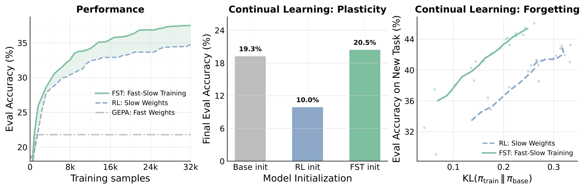
The experiments show three main results. First, the combined approach reaches the same accuracy as reinforcement learning alone with one-third to one-half as many training examples and then continues to a higher final accuracy ceiling. Second, at comparable performance the model parameters stay much closer to the original base model, with up to 70 percent lower divergence. Third, after training on one task the model retains the ability to learn a second, different task; pure reinforcement-learning checkpoints largely lose this capacity. In a continual-learning setting where tasks change every 200 steps, the joint method keeps acquiring new tasks while the parameter-only baseline stalls.

These outcomes matter because they show that post-training need not force every piece of task knowledge into the same fixed set of weights. By letting fast textual adaptations absorb transient, task-specific lessons, the slow parameters can focus on consolidating reusable skills, which preserves generality, data efficiency, and future learning capacity. This division of labor directly addresses the plasticity loss and forgetting problems that currently limit how long and how broadly a model can be improved after pre-training.

The authors recommend treating context optimization and parameter optimization as complementary channels that should be trained together rather than applied sequentially. Practical next steps include testing the framework with different prompt and weight optimizers, reducing the added compute cost of prompt updates, and exploring distillation routes that move fast-channel gains back into parameters when desired. They also flag the need for broader task coverage and more efficient reuse of rollouts.

The reported gains hold consistently across the three main task families and multiple held-out generalization suites, but the study uses one specific pair of optimizers and a modest set of model sizes and domains. Readers should therefore treat the exact efficiency multipliers and plasticity improvements as indicative rather than universal until further validation is available.

`

Learning, Fast and Slow: Towards LLMs That Adapt Continually

Rishabh Tiwari$^{}$ $^{1, 4}$ Kusha Sareen$^{}$ $^{2}$ Lakshya A Agrawal$^{*}$ $^{1}$
Joseph E. Gonzalez$^{1}$ Matei Zaharia$^{1}$ Kurt Keutzer$^{1}$ Inderjit S Dhillon$^{3}$
Rishabh Agarwal$^{\dagger}$ $^{2, 5}$ Devvrit Khatri$^{\dagger}$ $^{3, 6}$
$^{1}$UC Berkeley $^{2}$Mila $^{3}$UT Austin $^{4}$Eragon $^{5}$Periodic Labs $^{6}$Mirendil

Large language models (LLMs) are trained for downstream tasks by updating their parameters (e.g., via RL). However, updating parameters forces them to absorb task-specific information, which can result in catastrophic forgetting and loss of plasticity. In contrast, in-context learning with fixed LLM parameters can cheaply and rapidly adapt to task-specific requirements (e.g., prompt optimization), but cannot by itself typically match the performance gains available through updating LLM parameters. There is no good reason for restricting learning to being in-context or in-weights. Moreover, humans also likely learn at different time scales (e.g., System 1 vs 2). To this end, we introduce a fast-slow learning framework for LLMs, with model parameters as "slow" weights and optimized context as "fast" weights. These fast "weights" can learn from textual feedback to absorb the task-specific information, while allowing slow weights to stay closer to the base model and persist general reasoning behaviors. Fast-Slow Training (FST) is up to $3\times$ more sample-efficient than only slow learning (RL) across reasoning tasks, while consistently reaching a higher performance asymptote. Moreover, FST-trained models remain closer to the base LLM (up to $70%$ less KL divergence), resulting in less catastrophic forgetting than RL-training. This reduced drift also preserves plasticity: after training on one task, FST trained models adapt more effectively to a subsequent task than parameter-only trained models. In continual learning scenarios, where task domains change on the fly, FST continues to acquire each new task while parameter-only RL stalls.

Correspondence: {rishabhtiwari, lakshyaaagrawal}@berkeley.edu, [email protected], {devvrit.03, rishabhagarwal.467}@gmail.com

$^{*}$Equal contribution $^{\dagger}$Equal advising.

1. Introduction

Section Summary: Large language models are typically adapted to new tasks like math or coding by updating their internal parameters through reinforcement learning or fine-tuning, but this forces every improvement into the same fixed weights, which can reduce flexibility, cause forgetting of prior skills, and slow future learning. The paper proposes Fast-Slow Training, an approach that pairs these slow, persistent parameter updates with fast, cheap modifications to textual prompts and context that capture task-specific lessons without permanently altering the model. By letting the two components evolve together during training, the method achieves stronger performance with far less data while keeping the model closer to its original behavior and better able to learn new tasks later.

Large language models (LLMs) are commonly adapted through supervised finetuning (SFT) or reinforcement learning (RL), both of which modify the model parameters, to specialized domains such as math and coding [1, 2, 3, 4, 5]. However, treating parameter updates as the sole mechanism of adaptation creates a fundamental bottleneck: every improvement, whether it be a reusable reasoning skill, a task-specific heuristic or a transient lesson from recent rollouts, must be written into the same persistent set of model weights. Since the entire policy is parameterized by these weights, an update that improves in-domain reward simultaneously moves the model away from its base behavior [6, 7], reducing entropy [8, 9], hurting out-of-distribution generalization [5, 10, 11, 12], and degrading its ability to adapt to future tasks, known as plasticity loss [13, 14, 15, 16].

LLM systems also possess another powerful adaptation mechanism: prompts, instructions, and contextual information [17, 18]. Unlike model parameters, these textual components can be modified cheaply, frequently, and per task. Prompt optimization methods demonstrate that substantial behavioral improvements can be obtained by improving the textual context under which the model operates [19, 20, 21, 22, 23].

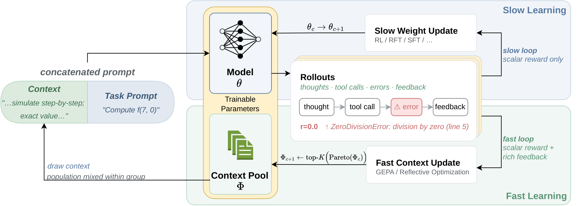
In this work, we introduce Fast-Slow Training (FST), where we view LLM adaptation as occurring through two complementary components (Figure 2). The first is a slow parametric component: the model weights, which are expensive to update, persist across tasks, and encode long-lived behavior. The second is a fast textual component: prompts, instructions, and task context, which can be changed cheaply and frequently, influence behavior immediately, capturing task-level adaptation without permanently modifying the model.

The fast-slow distinction we draw above has a long history in neural networks [24, 25, 26, 27], motivated by separating temporary, task-specific adaptations in fast-weights from persistent, broadly useful behaviors in slow-weights. We instantiate this idea in RLVR [3, 28] by interleaving slow reinforcement learning updates with fast context optimization using GEPA [23]. Rather than first training a policy and then optimizing a prompt for the final checkpoint, our method allows the context and the policy to co-evolve. The fast textual weights quickly incorporate lessons from rollouts, steering the model toward better reasoning behavior, while the slow parametric weights are updated under this evolving context. This produces a training process in which performance gains are distributed appropriately across both elements, instead of being forced entirely into the model parameters.

This division of labor has several consequences, which we evaluate in RLVR settings spanning math, code, and general reasoning tasks.

1. Fast textual adaptation improves data efficiency. Fast weights incorporate task-level signal rapidly, so the system improves without waiting for slow parameter updates. Empirically, fast-slow training matches RL reward with up to $3\times$ fewer rollouts and consistently reaches a higher performance ceiling (Section 4 Advantages 1 and 2).
2. Fast-slow training induces smaller slow-weight displacement. With the textual channel carrying part of the adaptation, the parameters need not move as far from the base policy. At matched reward, our models have up to 70% lower KL to the base policy than RL-only baselines. (Section 4 Advantage 3)
3. Fast-slow training preserves plasticity. We test this by training on one task using RL-only and FST, then continuing training on a second task from the resulting checkpoints; fast-slow trained models adapt effectively in the second phase while RL trained models collapse to near $0%$ - suggesting FST retains greater capacity for future learning (Figure 6 Advantage 4).
4. Fast-slow training enables continual learning. We test our method in setting where tasks change on the fly. We observe our method is able to adapt more quickly to changing objectives (Figure 7 Advantage 5).

Overall, our results suggest that effective LLM post-training should not be viewed as parameter learning followed by prompt tuning. Instead, it should be viewed as optimization over multiple adaptation channels, where fast textual weights and slow parametric weights are trained together to achieve rapid and task-specific improvements while preserving the generality and plasticity of the base model.

2. Preliminaries

Section Summary: This section introduces a framework that separates a model's fixed parameters, called slow weights, from adaptable textual prompts, called fast weights, which together shape how the model responds to queries. The overall goal is to jointly refine both elements by maximizing an expected reward across a distribution of tasks, where the model generates answers conditioned on a query and its current prompt. Slow weights are updated through reinforcement learning with verifiable rewards that compares groups of generated responses, while fast weights are evolved separately using an automated method that critiques and mutates prompts to improve performance on selected examples.

Fast and slow weights: a general framework

We model the slow weights (model parameters) as $\theta$, and fast weights (textual scaffolds) as $\phi$ drawn from a discrete text space $\Sigma^\ast$. Given a query $x$, the system produces a response by sampling

$ y \sim \pi_\theta(\cdot \mid x, \phi),\tag{1} $

where $\pi_\theta(y \mid x, \phi)$ denotes the policy induced by parameters $\theta$ when conditioned on textual context $\phi$ and query $x$. For a task distribution $\mathcal{D}$ and reward $r$, the natural joint objective is

$ \max_{\theta, \phi};; J(\theta, \phi) ;=; \mathbb{E}{x \sim \mathcal{D}, ; y \sim \pi\theta(\cdot \mid x, \phi)} ! \big[, r(x, y), \big].\tag{2} $

Each factor admits many concrete optimizers. On the slow side, $\theta$ can be updated by SFT, preference optimization [29], or policy-gradient methods such as PPO [30] and GRPO [3], frequently under verifiable rewards [2]. On the fast side, $\phi$ can be updated by automated prompt-optimization methods such as APE [19], OPRO [20], DSPy/MIPROv2 [21, 22], and GEPA [23]. Our framework is agnostic to these choices; we instantiate it with RL with verifiable rewards (RLVR) for $\theta$ and reflective evolutionary prompt optimization (GEPA) for $\phi$.

Slow weights: RL with verifiable rewards

We follow the ScaleRL recipe [28] for slow-weight updates. The reward $r(x, y) \in [0, 1]$ is given by an automatic verifier on $(x, y)$ [2] (e.g., rule-based correctness for math, code, and science tasks). For each query $x$, the current policy generates a group of $G$ rollouts ${y_i}_{i=1}^G$ under the current $(\theta, \phi)$, from which group-relative advantages [3] are computed,

$ A_i ;=; \frac{r(x, y_i) ;-; \bar{r}g}{\sigma_g ;+; \varepsilon}, \qquad \bar{r}g ;=; \tfrac{1}{G}!\sum{j=1}^{G} r(x, y_j), \qquad \sigma_g^2 ;=; \tfrac{1}{G}!\sum{j=1}^{G}!\big(r(x, y_j) - \bar{r}_g\big)^2,\tag{3} $

and normalized at the batch level. The policy is updated using the truncated importance-sampling REINFORCE objective $\textsc{cispo}$ [31, 28],

$ \mathcal{L}{\textsc{cispo}}(\theta) ;=; - \mathbb{E}!\left[ sg!\big(\min(\rho_t, \tau)\big) \cdot A \cdot \nabla\theta \log \pi_\theta(y_t \mid x, \phi, y_{<t}) \right],\tag{4} $

where $\rho_t = \pi_\theta(y_t \mid x, \phi, y_{<t}) / \pi_{\theta_{\text{old}}}(y_t \mid x, \phi, y_{<t})$ is the per-token importance ratio between the current and behavior policies, $\tau$ is a truncation threshold, $\mathrm{sg}(\cdot)$ is the stop-gradient operator, and the loss is aggregated at the prompt level. In conventional RLVR training, $\phi$ is fixed to a generic system prompt and only $\theta$ is updated.

Fast weights: reflective prompt evolution.

We optimize the fast weights $\phi$ using GEPA [23], a reflective evolutionary procedure over textual prompts $\phi \in \Sigma^\ast$. For a fixed policy $\pi_\theta$, the fitness of a prompt on instance $x$ is its expected reward,

$ s(\phi; x) ;=; \mathbb{E}{y \sim \pi\theta(\cdot \mid x, \phi)} !\left[r(x, y) \right].\tag{5} $

GEPA maintains a population of prompts, uses rollouts to elicit natural-language critiques from a frozen reflection LM, and proposes textual mutations that improve performance on an anchor set from $\mathcal{D}$. Rather than returning a single prompt, GEPA retains a Pareto frontier of complementary prompts and returns the top- $m$ candidates, which we use as fast weights. We defer the details of parent selection, mutation, pruning, and prompt examples to Appendix A.

3. Fast-Slow Training (FST)

Section Summary: Fast-Slow Training alternates between refining a language model’s core parameters with reinforcement learning and periodically refreshing a population of prompts. At the start of each cycle, it uses GEPA on a batch of recent examples to produce a small set of complementary prompts that perform well on different subsets of the data. It then fixes this prompt population and runs several RL updates, mixing rollouts from each prompt within the same problem group so that the advantage calculation reflects both prompt-induced and sampling-induced variation.

We now describe $\textsc{FST}$, which jointly optimizes slow weights $\theta$ through RL and fast weights $\Phi$ through GEPA. The method maintains a population of $K$ textual prompts, $\Phi={\phi^{(1)}, \ldots, \phi^{(K)}}$, and optimizes

$ \max_{\theta, \Phi};; J(\theta, \Phi)

\mathbb{E}{x\sim\mathcal{D}, ;\phi\sim U(\Phi), ;y\sim\pi\theta(\cdot\mid x, \phi)} !\left[r(x, y)\right],\tag{6} $

where $U(\Phi)$ is uniform over the prompt population. We keep a population rather than a single best prompt because GEPA returns a Pareto frontier of complementary prompts: different prompts perform best on different subsets of $\mathcal{D}$. Sampling across this frontier during RL gives the policy access to multiple conditioning behaviors and lets group-relative advantages compare both prompt-induced and sampling-induced variation on the same problem. Training proceeds in cycles of $T$ slow-weight updates. At the start of cycle $c$, we pre-fetch the next $T$ RL batches and denote their union by the lookahead batch $\mathcal{L}c$. We run GEPA with the current policy $\pi{\theta_c}$ as the rollout model, a frozen reflection LM $\pi_{\mathrm{ref}}$ as the proposer, $\mathcal{L}c$ or a fixed-size subset as the anchor set, and the previous population $\Phi_c$ as the seed. GEPA returns the top- $K$ candidates from its Pareto frontier, yielding the fast weights $\Phi{c+1}$. For the next $T$ steps, we update $\theta$ on minibatches from $\mathcal{L}c$ while holding $\Phi{c+1}$ fixed. For each problem $p$, we form a rollout group of size $G$ by sampling each prompt $\phi^{(k)}\in\Phi_{c+1}$ exactly $G/K$ times. That is, in each group, $G/K$ rollouts receive the same prompts and we have $K$ such mini-groups. Cumulatively, they are treated as one group for $p$; rewards are normalized by the per-problem statistics $(\bar{r}_g, \sigma_g)$ as in eq Equation 3, mixing prompt and sampling variation within the same advantage computation. We then apply the $\textsc{cispo}$ update in Equation 4. After $T$ updates, the procedure repeats with a new GEPA phase under the updated policy. Pseudocode of $\textsc{FST}$ is given in Appendix B.

4. Advantages of Fast-Slow Training

Section Summary: Fast-slow training lets a model handle new tasks by making small, temporary adjustments through short textual prompts while leaving its core parameters largely unchanged. Because the permanent weights shift less than they would under ordinary reinforcement learning, the approach reaches strong performance after fewer training examples, settles at a higher accuracy level, and stays closer to the original model. These changes also preserve the model's ability to learn later tasks without interference.

The textual fast weights $\Phi$ carry part of the task-level information that RL would otherwise force into $\theta$, so the slow weights move less to reach the same reward. The downstream signature of this division of labor is consistent across our settings: training reaches matched reward more quickly, $\theta$ drifts less from the base policy at convergence, the model retains greater plasticity to adapt to subsequent tasks, and our method shows higher continual learning capability. We show each of these in the following sections. Advantage 1: Fast-Slow Training Improves Data Efficiency 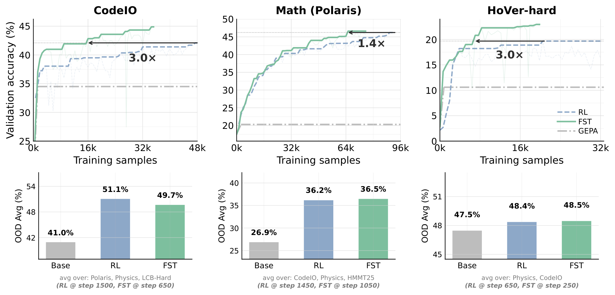We evaluate $\textsc{FST}$ on three training families: code-output prediction (CodeIO) [32, 33], math (Polaris) [34], and multi-hop fact verification (HoVer-hard) [35]. All experiments use Qwen3-8B [36], except for the Math run, where we first SFT Qwen3-8B-Base on Nemotron data [37] because Qwen3-8B is already saturated on math benchmarks. $\textsc{FST}$ uses cycle length $T{=}6$ and $K \in {4, 8}$ candidate prompts per cycle. Training-time performance is measured on a held-out in-distribution validation set. RL is trained until step $1500$ or in-distribution saturation (whichever comes first); $\textsc{FST}$ is trained at least until it matches RL's running peak. Full hyperparameters and dataset details are deferred to Appendix D. The matched-step training curves (Figure 3 Top) show that $\textsc{FST}$ reaches RL's running peak in substantially fewer optimizer steps: $\mathbf{3.0\times}$ fewer on CodeIO , $\mathbf{1.4\times}$ on Math , and $\mathbf{3.0\times}$ on HoVer-hard. Continuing past the crossover, $\textsc{FST}$ 's running peak also exceeds RL's on all three tasks . To check that the in-distribution data efficiency does not come at the cost of out-of-distribution behavior, for each training task we compare Base, RL's final checkpoint, and $\textsc{FST}$ 's validation matched-performance checkpoint on a family of cross-domain and easy-to-hard generalization datasets, with no GEPA prompt at inference (Figure 3 bottom). Across all three training families, the OOD average is essentially flat between $\textsc{FST}$ and RL ($-1.4$, $+0.3$, $+0.1$ pp on CodeIO, Math (Polaris), and HoVer-hard respectively) despite $\textsc{FST}$ reaching the in-distribution peak in $1.4\times$ to $3.0\times$ fewer training samples. Concretely, $\textsc{FST}$ reaches $49.7%$ versus RL's $51.1%$ on CodeIO-trained OOD (avg over Polaris, Physics, LCB-Hard), $36.5%$ versus $36.2%$ on Math-trained OOD (avg over CodeIO, Physics, HMMT25), and $48.5%$ versus $48.4%$ on HoVer-hard-trained OOD (avg over Physics, CodeIO). All three are well above the corresponding Base reference ($41.0%$, $26.9%$, $47.5%$). The in-distribution data-efficiency advantage therefore comes at no measurable cost in out-of-distribution behavior. Advantage 2: Fast-Slow Training Raises the Performance Asymptote 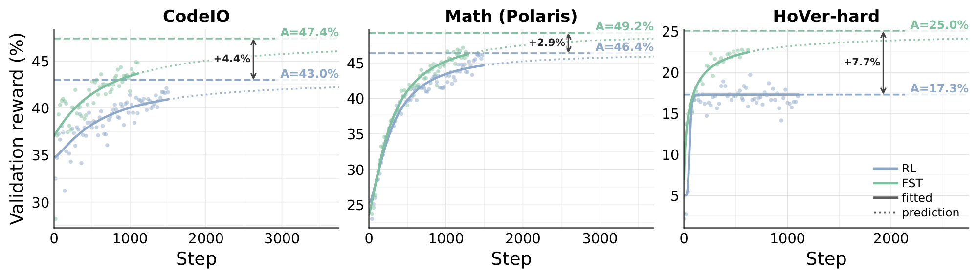Following [28], we compare RL and $\textsc{FST}$ by the saturation level of their validation-accuracy curves rather than at any single training step. Unlike final-step or matched-step accuracy, which depends on where each run was stopped, the asymptote of a fitted curve reads off the level the run is converging to. For each (task, method) we fit a sigmoid curve

$ \Delta R = \frac{A - R_0}{1 + (C_{mid}/C)^B} $

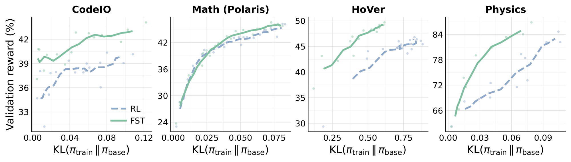
to the validation-accuracy trajectory, where $A$ is the upper asymptote, $B$ a scaling exponent, $C_{mid}$ the midpoint of the performance, and $R_0$ is the initial reward at step 0. Across all three tasks (Figure 4), $\textsc{FST}$ 's fitted asymptote exceeds RL's: $A{=}47.4%$ vs $43.0%$ on CodeIO ($+4.4$ pp), $49.2%$ vs $46.4%$ on Math (Polaris) ($+2.9$ pp), and $25.0%$ vs $17.3%$ on HoVer-hard ($+7.7$ pp). Pushing part of the task adaptation into the textual fast-weight channel $\Phi$ in addition to the slow weights $\theta$ helps the overall method converge to a higher accuracy ceiling than RL alone reaches. Advantage 3: Fast-Slow Training Remains Close to the Base Model 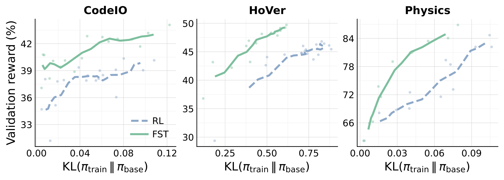The KL divergence $\mathrm{KL}(\pi_{\text{train}}, |, \pi_{\text{base}})$ between the post-trained policy and the base measures how far the slow weights have moved away from their base configuration; larger displacement is associated with reduced entropy, weaker OOD generalization, and lower plasticity for future tasks [13, 14, 15, 16]. We track this directly - at each training checkpoint we compute token-level KL from the base on the held-out validation prompts and plot it against the same checkpoint's validation accuracy, for both $\textsc{FST}$ and RL across Physics, Math (Polaris), HoVer, and CodeIO. Across all four tasks (Figure 5), $\textsc{FST}$ achieves higher performance at lower KL than RL. [38] recently showed that on-policy RL is already biased toward KL-minimal solutions on a new task, and that the size of this shift correlates with how much prior knowledge is forgotten. Even relative to this strong baseline, $\textsc{FST}$ shifts the accuracy/KL frontier further left. We next demonstrate that this reduced displacement preserves plasticity and enables continual learning in the models trained with $\textsc{FST}$. Advantage 4: Fast-Slow Training Preserves Plasticity 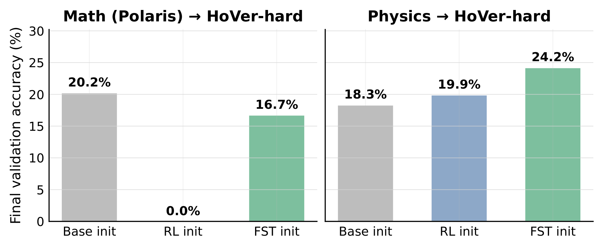Continued post-training has been observed to hamper a model's ability to learn future tasks, a phenomenon commonly called plasticity loss [15, 14, 13, 16]: the slow weights become specialized to the trained task and lose responsiveness to gradient signals from new ones. We probe this directly in two phases. Phase 1 trains a base model on task $X$ using either standard RL or $\textsc{FST}$. Phase 2 takes the Phase-1 checkpoint as initialization and runs standard RL on a different task $Y$. Throughout Phase 2 we track validation accuracy on $Y$. As a no-prior-training reference, we also run Phase 2 starting from the base model. We test $\texttt{Math} \to \texttt{HoVer-hard}$ and $\texttt{Physics} \to \texttt{HoVer-hard}$. Figure 6 shows that in Phase-2, $\textsc{FST}$-init outperforms RL-init through the 400-step probe in both settings. The contrast is sharpest in Math $\to$ HoVer-hard: prior RL collapses HoVer-hard learnability to near-zero, the RL-init curve drops to $\sim 0%$ within 40 steps and stays flat for the rest of the run. In contrast, $\textsc{FST}$-init reaches performance close to the base-init reference. On Physics $\to$ HoVer-hard, $\textsc{FST}$-init finishes at $24.2%$ and is still climbing, versus RL-init's $19.9%$ at step 400 . This indicates that, unlike RL, $\textsc{FST}$ does not over-specialize the slow weights to task $X$: the resulting checkpoint retains capacity to learn a new task $Y$, exhibiting higher plasticity. Advantage 5: Fast-Slow Training Improves Continual Learning 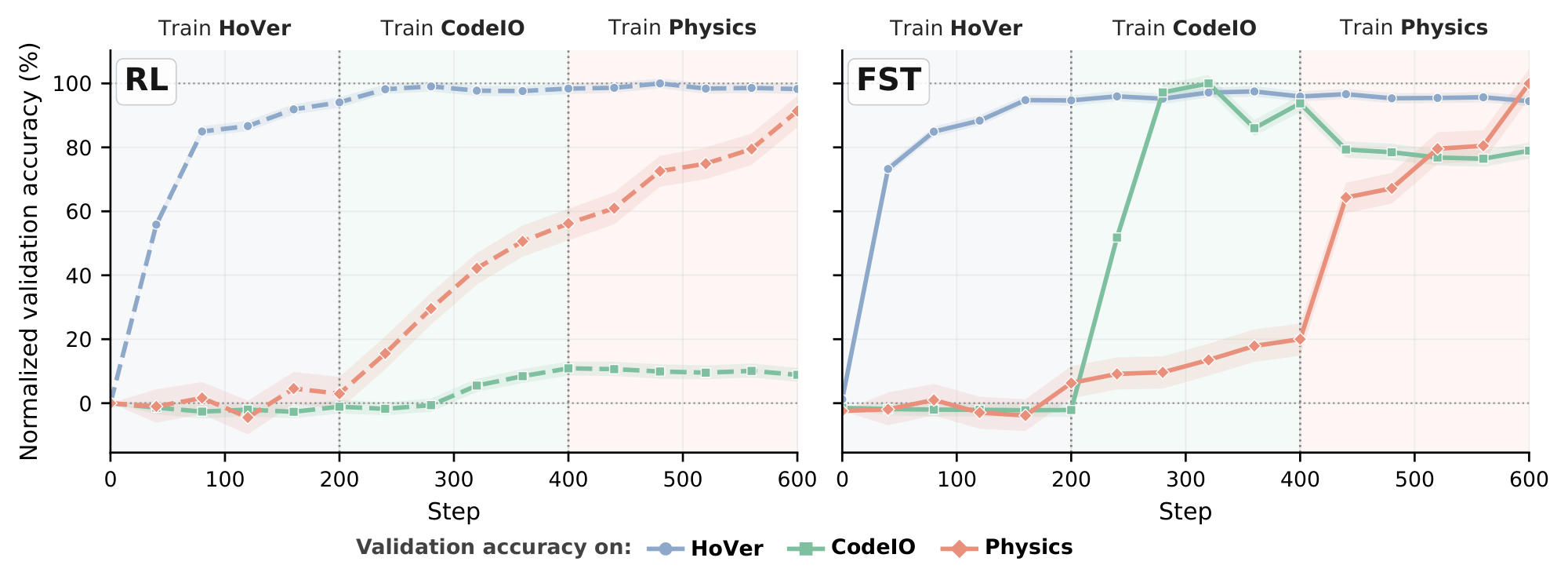A continual learning algorithm must keep absorbing new tasks as training proceeds, without losing the capacity to absorb later ones [15, 16, 14]. To test this we run a single uninterrupted training pass over three tasks, sequentially swapping the task every 200 steps - first 200 steps with HoVer (multi-hop fact verification), then CodeIO (code-output prediction), and finally Physics (multiple-choice from sciknoweval). In this setting, the same live training trajectory must absorb three task changes back-to-back, mirroring how a deployed model would actually be trained on a stream of incoming tasks. Figure 7 shows evaluation on all three tasks at different points across the full 600-step training run, normalized within each stage so that $0$ is the stage's starting accuracy and $100%$ is peak performance on the task across methods. $\textsc{FST}$ reaches near-peak in every stage while learning faster within each stage, mirroring the data-efficiency gap of Section 4 Advantage 1. The contrast is sharpest in the second stage, CodeIO: across the full 200-step budget, RL barely lifts off its starting accuracy, peaking at $20.7%$ mean@16 (a $+2.5$ pp gain over its $18.3%$ stage-start), while $\textsc{FST}$ climbs to near-peak in just $\sim$ 80 steps (less than half the budget) and finishes the stage at $37.7%$, a $+19.6$ pp gain (a $\sim 8\times$ within-stage acquisition rate over RL, and a $+17.0$ pp absolute lead at step 400). This demonstrates that $\textsc{FST}$ is a promising continual-learning algorithm for LLMs: by routing task-level adaptation through both the textual fast-weight channel $\Phi$ in addition to $\theta$, the method remains capable of acquiring later tasks under continued optimization.

5. Why Does Fast-Slow Training Work?

Section Summary: Fast-slow training succeeds because the fast component can extract useful task patterns and feedback from just a handful of examples, producing measurable improvements within dozens of steps instead of the hundreds required for ordinary weight updates to begin registering gains. At the same time, allowing both the fast prompts and the slow model parameters to optimize directly against the same reward signal lets each task draw on whichever channel delivers value, and their combination reliably lifts final performance beyond what either achieves alone. Pure distillation from fast to slow weights falls short of this joint optimization, confirming that the two channels must work together throughout training.

The empirical benefits in Section 4 raise the questions: where do the benefits come from exactly and which component is doing the majority of the work in which setting? The two studies below isolate these questions. Observation 1: Fast Weights Acquire Task Signal Faster Than Slow Weights 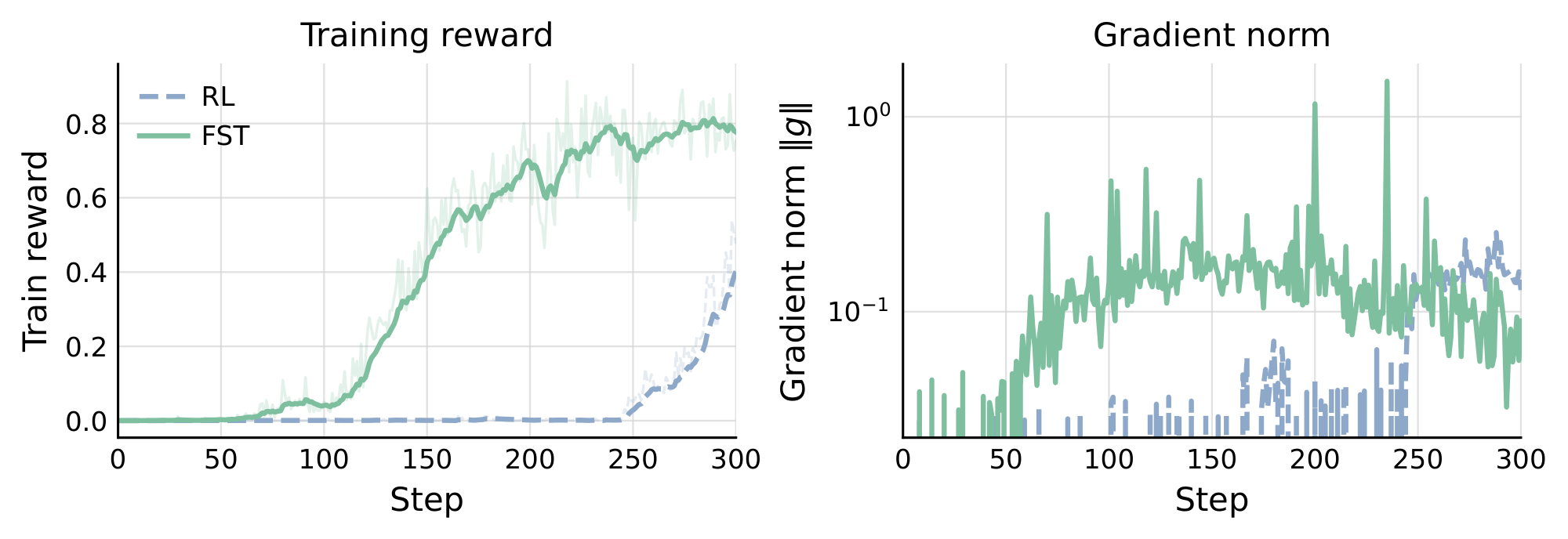To explore how $\textsc{FST}$ and RL behave when the base model obtains near-zero rewards, we run both $\textsc{FST}$ and an RL baseline on a synthetic star-graph reasoning task. Given a star-shaped graph in context, the goal is to find a path between two labeled nodes. The two methods exhibit qualitatively different early-training behavior (Figure 8). Parameter-only RL produces near-zero reward for roughly the first $\sim$ 300 steps before reward begins to rise. In contrast, $\textsc{FST}$ reaches measurable reward by around step $\sim$ 50, driven almost entirely by the first few GEPA cycles, before $\theta$ has had time to move appreciably. This is heightened by the ability of $\textsc{FST}$ to leverage text feedback. The task provides informative feedback on failures, detailing where exactly a submitted path went wrong. The interpretation is direct: slow weights are slow in how many updates they require to begin moving signal at all. The fast channel does not have this latency: GEPA can extract task structure from a handful of rollouts and inject it through $\Phi$ immediately. While GEPA alone only aids in solving a few problems early on, it provides enough gradient signal for FST to climb rewards quickly. 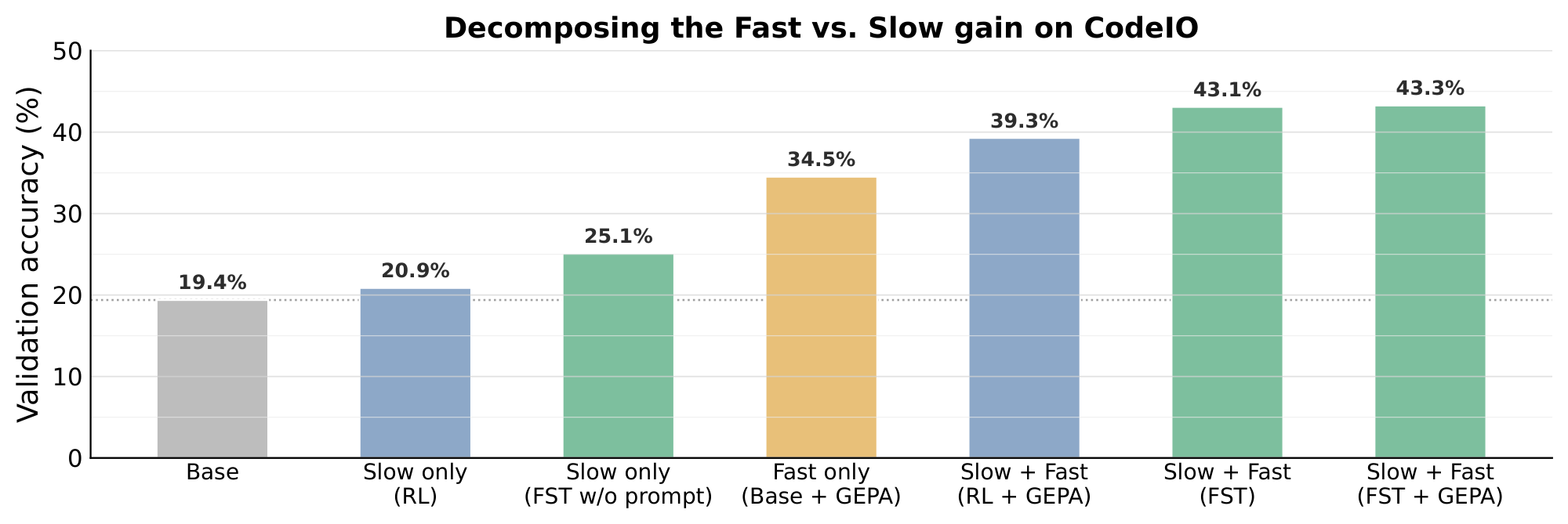Observation 2: Fast and Slow Weights Both Optimizing for Reward Raise Performance Ceiling 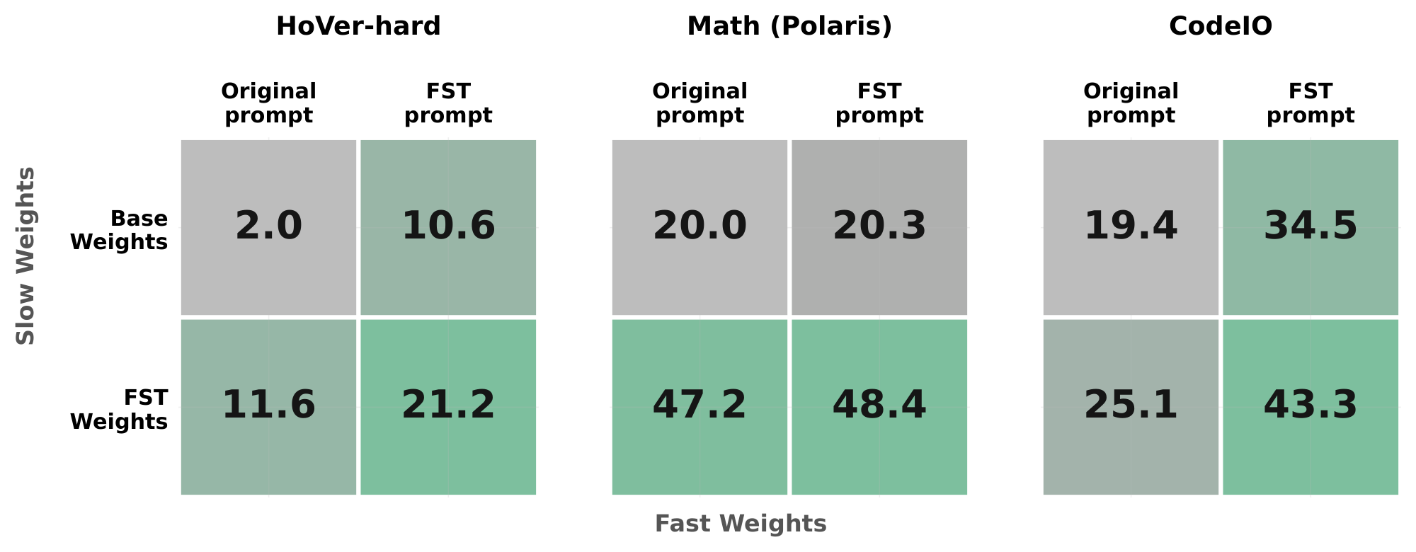Figure 9 decomposes the in-distribution gain on each training task into slow-weight and fast-weight contributions, evaluating every combination of base, $\textsc{FST}$-trained weights with original prompt, $\textsc{FST}$-evolved prompt. On HoVer-hard, the slow channel alone lifts pass@1 from $2.0%$ to $11.6%$, the fast channel alone lifts it to $10.6%$, and combining the two reaches $21.2%$. The same pattern holds on CodeIO, where the joint cell reaches $43.3%$ versus $25.1%$ (slow only) and $34.5%$ (fast only); a finer-grained CodeIO decomposition appears in Figure 14. On Math (Polaris) almost all of the gain is carried by the slow weights ($20.0 \to 47.2$), consistent with the weaker instruction-following of the custom SFT base used for Polaris (see Appendix G). $\textsc{FST}$ does not assume a fixed division of labor between the two channels, and lets each task draw on whichever channel pays off while still combining them when both contribute. In Appendix H we further ask whether an explicit fast-to-slow distillation algorithm can substitute for direct RL on the slow weights. Our initial results using naive distillation suggest that it cannot. Distillation alone plateaus well below $\textsc{FST}$, confirming that both channels need to optimize against reward jointly to lift the ceiling.

6. Discussion

Section Summary: Training models with separate fast and slow updates lets them acquire new skills through context changes rather than overwriting their core knowledge, which preserves prior abilities and supports ongoing learning across varied tasks. This setup also enables more efficient improvement by incorporating richer text-based feedback during updates and maintains training variety through a broad range of prompts. The overall approach remains generalizable, though future efforts could focus on greater computational efficiency, broader testing of optimization techniques, and expanded use in distilling knowledge from examples.

In Section 4 and Section 5, we describe several benefits of training reasoning models with fast-slow updates. As models with finite capacity are trained across ever more diverse sets of environments, we argue that not all task-specific information need be distilled in the weights of the model. We observe some encouraging properties of the new paradigm. First and foremost, $\textsc{FST}$ maintains proximity to the base model, enabling a set of features suitable to continual learning: plasticity and lack of forgetting. Secondly, the framework allows for data efficient learning, in part due to the ability to learn from text feedback in the context update, overcoming the widely accepted 1-bit-per-episode information limit of binary RLVR. Finally, we observe healthy diversity during training due to a wide prompt pool. The distinction between context and weight optimization represents a broader split between declarative and procedural knowledge, an important distinction for any general-purpose reasoner.

6.1 Limitations and future work

While this study focuses primarily on investigating a particular instantiation of the fast-slow paradigm, taking CISPO and GEPA as highly capable methods for weight and prompt optimization, the framework is highly general. Studying the impact of changing the prompt or the weight optimizer is an interesting avenue for future work. Additionally, we believe there is potential to make the method more compute efficient and better reuse trajectories across prompt and weight optimization. Finally, though we present an initial exploration of applying this paradigm to distillation-based approaches in Figure 13, we believe a more comprehensive study of this direction to be an exciting avenue for future work.

7. Related Work

Section Summary: Researchers have explored two main ways to improve large language models on reasoning tasks. One approach uses reinforcement learning to gradually update the model’s internal parameters, but this can reduce the model’s flexibility over time. A complementary line of work focuses on quickly refining the text prompts or context the model sees without changing its weights, an idea inspired by neuroscience theories of fast and slow learning systems. Recent studies have begun combining both strategies, and this section positions the current method as an interleaved approach that maintains a population of evolving prompts alongside ongoing parameter updates.

Slow learning: RL for LLM reasoning. Verifiable-reward LLM post-training writes every improvement into the model parameters via policy-gradient methods such as PPO, DPO, GRPO, and CISPO ([30, 29, 3, 31]), used in most reasoning-RL pipelines ([2, 28, 36]). Prolonged parametric adaptation shrinks output entropy, raises KL to the base policy, and erodes the model's ability to absorb new tasks, called the plasticity loss phenomenon ([15, 14, 13, 16, 38]). We share this diagnosis but add a fast textual channel that absorbs much of the task-specific adaptation the slow weights would otherwise carry. Fast learning: prompt and context optimization. A parallel literature shows that substantial behavioral gains can come from editing the textual context alone, via discrete-prompt search ([39, 40, 41]), LLM-driven prompt proposers ([19, 20, 42, 43]), evolutionary methods ([44, 45, 46]), compound LM programs ([21, 22, 47, 48, 49, 50]), evolving agent context ([51, 52, 53, 54]), and reflective self-feedback ([55, 56, 23]). We use GEPA, which maintains a per-instance Pareto frontier of candidate prompts. All these methods are typically applied post-hoc to a frozen checkpoint, leaving the slow and fast channels disjoint in time. Fast and slow weights: complementary learning systems. The fast/slow decomposition predates deep learning, with roots in the neuroscience of complementary learning systems ([57, 58]) and a long line of fast-weight architectures and dual-timescale learners in neural networks ([24, 25, 26, 59, 60, 61]). We adopt this decomposition for LLM post-training, instantiating the fast channel as an evolving population of textual prompts and the slow channel as the model parameters. Modern fast–slow methods for LLM RL. A small but growing body of work combines textual feedback with reward-driven weight updates. BetterTogether ([62]) alternates SFT with prompt optimization over a DSPy pipeline, albeit instantiated with prompt optimizers that don't use textual feedback; we extend this to a new training paradigm instantiated in verifiable-reward RL in which a Pareto-frontier prompt population created with textual feedback co-evolves with the policy. LANPO ([63]) interleaves language and numerical feedback via per-instance reflections; we instead maintain a cross-problem Pareto-frontier population. Recent work E-SPL ([64]) explores prompt optimization and RL at a smaller scale with focus on performance rather than adaptation. mmGRPO ([65]) runs prompt optimization once and then RL on a DSPy program; we interleave the two across cycles. POPE ([66]) prefixes hard prompts with partial reference solutions; $\textsc{FST}$ learns task-level prompts that condition any rollout, and combining the two is a natural direction for future work.

8. Conclusion

Section Summary: The paper introduces a fast-slow post-training approach for large language models that updates the model's core parameters gradually through reinforcement learning while separately evolving a set of helpful text instructions to guide it. Experiments on coding, math, and fact-verification tasks show this combined method reaches strong results with far fewer training steps than standard reinforcement learning, achieves higher final performance, and leaves the model better able to learn new tasks later. The work argues that splitting adaptations between fixed model weights and changeable text prompts can make training more efficient and less harmful to the model's long-term flexibility.

We present a fast-slow framework for LLM post-training that jointly optimizes the slow model parameters $\theta$ via RL and a fast textual-context population $\Phi$ via reflective prompt evolution, interleaving the two channels. Across CodeIO, Math, and HoVer-hard, this co-optimization reaches matched performance with $1.4$ – $3\times$ fewer optimizer steps, attains a higher asymptote, and incurs lower KL displacement than RL alone, which in turn translates into preserved plasticity and stronger continual-learning behavior on new tasks. More broadly, our results suggest that effective post-training should not ask model parameters to absorb all forms of adaptation. Fast textual weights can capture task-specific and rapidly evolving improvements, while slow weights can focus on consolidating persistent behavior. This division of labor offers a path toward post-training methods that are more data-efficient, less destructive, and more amenable to continual learning.

9. Acknowledgements

Section Summary: The authors thank a range of companies and research organizations, including Furiosa AI, Apple, NVIDIA, Google, Amazon, and others, for financial support, computing resources, and technical help that made the work possible. They also recognize individual colleagues for useful conversations and infrastructure assistance, along with fellowship funding for one team member. The section closes by noting that the paper’s conclusions are the authors’ own and do not reflect the views of any sponsors.

The authors acknowledge the gracious support from the Furiosa AI, Apple, NVIDIA, Macronix, Mozilla team, Open Philanthropy / Coefficient Giving, and Amazon Research. Furthermore, we appreciate the support from Google Cloud, the Google TRC team Prof. David Patterson, along with support from Google Gemini team, and Divy Thakkar. Lakshya A Agrawal is also supported by a Laude Slingshot grant and Laude residency provided by the Laude Institute and an Amazon AI PhD Fellowship. We would like to thank Harman Singh, Nishanth Anand and Reza Bayat for useful discussions related to continual learning. Finally, the authors would also like to thank Josh Sirota and the Eragon team for infrastructure and compute support. Our conclusions do not necessarily reflect the position or the policy of our sponsors, and no official endorsement should be inferred.

Appendix

Section Summary: The appendix describes GEPA, an evolutionary search procedure that maintains a population of prompt variants and uses a separate reflection language model to critique rollouts and propose textual mutations, selecting parents from a per-instance Pareto frontier to preserve useful diversity. It then presents pseudocode for the overall FST training loop, which alternates blocks of group-relative policy optimization on minibatches with periodic GEPA-driven prompt evolution over successive data cycles. The final subsection explains how the star-graph dataset is procedurally generated as a hard path-finding task on synthetic graphs with a high-degree source node and many decoy branches, along with the fixed prompt template and exact-match reward used for evaluation.

A. GEPA

We optimize the fast weights $\phi$ using GEPA [23], a reflective evolutionary procedure that searches the text space $\Sigma^\ast$ guided by a frozen reflection LM $\pi_{\text{ref}}$, a separate capable model that proposes textual mutations from natural-language critiques of rollouts. For a candidate $\phi$ and query $x$, define the per-instance fitness

$ s(\phi; x) ;=; \mathbb{E}{y \sim \pi\theta(\cdot \mid x, \phi)}!\big[, r(x, y), \big].\tag{5} $

GEPA maintains a population $\mathcal{P}$ of candidate prompts whose fitness vectors (s(phi; $x_1)$, ..., s(phi; $x_n))$ on an anchor set $x_i$ for i=1..n drawn from D are tracked. One generation proceeds in four steps: (i) select a parent $\phi_p$ from the per-instance Pareto frontier of $\mathcal{P}$; (ii) sample a minibatch of rollouts under $\phi_p$ from $\pi_\theta$; (iii) elicit a child $\phi_c \leftarrow \pi_{\text{ref}}!\big(\phi_p, , \text{traces}\big)$ by having the reflection LM diagnose failures and propose a textual edit; (iv) evaluate $s(\phi_c; \cdot)$ on the anchor set, add $\phi_c$ to $\mathcal{P}$, and prune dominated candidates. After a fixed metric-call budget, GEPA returns the top- $m$ candidates of the resulting Pareto frontier. The frontier preserves diversity: different candidates are best on different slices of $\mathcal{D}$, and this diversity is precisely what allows the RL phase to exploit several complementary fast weights simultaneously. GEPA is related to other LLM-as-optimizer methods that use natural-language reflection or self-feedback [55, 56, 20], and is distinguished by its per-instance Pareto population and explicit prompt-mutation operator.

B. Algorithm pseudocode

We present the algorithm pseudocode in Algorithm 1.

**Require:** initial slow weights θ₀; seed prompt φ(seed); data stream D; cycle length T; population size K; GRPO group size G with K | G; reflection LM π(ref) Φ₀ ← {φ(seed) **for** cycle c = 0, 1, 2, … **do** L(c) ← pre-fetch the next T minibatches from D // lookahead batch Φ(c+1) ← GEPA (π_θ(c), π(ref), L(c), Φ(c), K) **for** t = 1, …, T **do** sample minibatch B(t) ⊂ L(c) **for all** p ∈ B(t) **do** **for all** φ(k) ∈ Φ(c+1) **do** assemble G/K rollouts under (p, φ(k)), sampling from π_θ(· | p, φ(k)) **end for** place all G rollouts in one group; compute group-relative advantages **end for** update θ with L(CISPO) (Eq. 4) **end for** **end for**

C. Star-graph dataset construction

Star-graph search is a planning task introduced by [67]. We adopt their problem definition and procedurally generate our train and test splits.

Graph instance.

Each instance is parameterized by a triple $(d, p, n)$: source degree $d$, path length $p$, and node-pool size $n$. We sample without replacement from ${0, 1, \ldots, n-1}$ to draw the source $s$ and goal $g$ ($s \neq g$), then $p-2$ distinct intermediate nodes that together form the unique gold path $s !\to! v_1 !\to! \cdots !\to! v_{p-2} !\to! g$ (yielding $p-1$ edges of length 1 each). On top of the gold path we attach $d-1$ decoy branches rooted at $s$, each itself a chain of length $p$, with all decoy nodes drawn fresh from the unused pool so that no decoy intersects the gold path or another decoy. The full edge set is then shuffled uniformly at random and serialized as a flat space-separated list of comma-separated pairs. The graph is treated as undirected at scoring time but presented as a list with no ordering hint.

Why this is a hard exploration problem.

The source $s$ is the only node with degree $d$; every other node sits on a chain and has degree $2$ (its predecessor and successor along that arm). The first hop is therefore the only real branching decision: picking a decoy arm commits the model to a chain that never reaches $g$, and the path-listing output format gives no built-in way to backtrack. With $d=25$ a uniformly-random first hop would succeed only $4%$ of the time, and empirically Qwen3-4B-Instruct does worse than uniform: pass@ $16$ is $0/50$ on the seed prompt before any RL update, because the model's strong path-finding prior is miscalibrated for this synthetic layout and concentrates probability on a wrong arm. This is the ``RL stuck at zero'' regime that motivates fast-weight prompt evolution.

Prompt template.

Every example is formatted with the verbatim template from the original reference implementation:

Given a bi-directional graph in the form of space separated edges, output a path from source node to the destination node in the form of comma separated integers.

For this question the graph is graph

The source node is source

The destination node is destination

Please reason step by step, and put your final answer within \boxed.

The seed system prompt used during RL and as the initial GEPA candidate is:

You are solving a graph path-finding task. You will be given a list of edges and a source and destination node. Output one valid path from source to destination. Inspect the source node's neighbors first, identify which neighbor leads to the destination via a sequence of valid edges, then commit to that branch. Each consecutive pair in your output path must be a valid edge in the graph. Put your final answer comma-separated inside boxed braces.

Scoring.

The reward function extracts the contents of the last \ boxed{…} from the post-</think> body of the rollout, strips whitespace, and applies an exact-match comparison against the gold path $s, v_1, \ldots, v_{p-2}, g$ rendered as a comma-separated string. The reward is $1.0$ on exact match and $0.0$ otherwise. The task admits no partial credit, so even a single wrong intermediate node zeros the reward.

Splits used in the paper.

We sweep difficulty by varying $(d, p, n)$. The headline experiments use $(d, p, n) = (25, 20, 500)$ with $10{,}000$ training examples and $200$ held-out test examples.

D. Hyperparameters and compute

This appendix lists all training hyperparameters needed to reproduce the numbers in the main paper. Settings shared across domains are described first; per-domain overrides follow in Table 1--Table 2.

Shared RL configuration.

All RL runs are GRPO ([3]) with the $\textsc{cispo}$ surrogate loss ([31, 28]) ($\text{clip_low}=1.0$, $\text{clip_high}=3.0$), advantage normalization by per-group standard deviation, and a small KL-to-reference penalty ($\text{coef}=10^{-3}$). The actor optimizer is AdamW (PyTorch defaults $\beta_1=0.9$, $\beta_2=0.999$, weight decay $0$) at learning rate $10^{-6}$ with a $10$-step linear warm-up; we use no learning-rate decay. Each RL step samples $G=8$ rollouts per problem with train_batch_size $, =32$ problems (so $256$ rollouts per step), runs PPO updates with ppo_mini_batch_size $, =32$, and uses tensor-parallel size $1$ for the rollout engine (vLLM). At evaluation time we report mean@ $4$ over four rollouts per validation prompt at temperature $0.6$, top- $p$ $0.95$. We checkpoint every $50$ training steps and keep all checkpoints. All runs use Qwen3 thinking mode except star-graph (which uses the Instruct base, no thinking) and the no-thinking baselines reported in the main text.

Shared GEPA configuration.

GEPA cycles use the same settings for all domains: cycle length $T=6$ RL steps between GEPA optimizations (equivalently, $\texttt{warmstart_steps}=\texttt{rl_steps_per_cycle}=6$); all $K$ population prompts are scored on every question (prompts_per_question $, =K$) with advantage grouping Option B (advantage_grouping="question"), so a problem's $G$ rollouts are split $G/K$ per prompt and a single group statistic $(\bar{r}_g, \sigma_g)$ is computed across all of them. The reflection LM is OpenAI gpt-5.2, accessed through LiteLLM. Per-cycle GEPA budgets are $\texttt{num_eval_examples}=192$ and $\texttt{max_metric_calls}=960$ across all domains except polaris ($96$ and $1500$) and star-graph ($200$ and $960$). Candidate prompts are injected as a system message; for datasets whose raw prompt already contains a system message (HoVer, Physics, Math) we merge the GEPA prompt into the existing system role rather than stack a second one. Each GEPA cycle outputs a Pareto-frontier population of size $K$ which seeds the next cycle.

Per-domain overrides.

Table 1 and Table 2 summarize the parameters that vary across training domains.

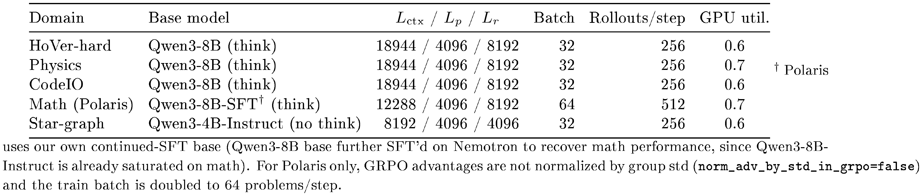
::: {caption="Table 1: Per-domain RL hyperparameters and base models. $L_c$ tx / $L_p / L_r$ are the maximum context, prompt, and response lengths (tokens). Train batch is the number of problems per RL step; rollouts/step is batch × G."}

:::

: Table 2: Per-domain GEPA hyperparameters. $K$ is the population size; $G/K$ is the number of rollouts each candidate prompt produces per problem within an RL group. Eval set / metric calls are the per-cycle GEPA budgets.

Domain	$K$	$G/K$	Cycle $T$	Eval set	Metric calls	Reflection LM
HoVer-hard	8	1	6	192	960	gpt-5.2
Physics	4	2	6	192	960	gpt-5.2
CodeIO	8	1	6	192	960	gpt-5.2
Math (Polaris)	4	2	6	96	1500	gpt-5.2
Star-graph	8	1	6	200	960	gpt-5.2

Compute and wall-clock.

All runs are submitted to a SLURM cluster with $8 \times$ H100 (80GB) per node. The headline runs in the main paper are single-node ($1\times8$ GPU); the Polaris $K=8$ ablation is the only multi-node configuration ($4\times8 = 32$ GPUs). Mean per-RL-step wall-clock under the headline configuration is $\sim 60$ s for RL-only and $\sim 100$ s for $\textsc{FST}$ without rollout reuse (HoVer-hard, $K=8$). Enabling rollout reuse (Appendix F) brings the RL-step cost down to $\sim 47$ s, slightly faster than RL-only at the step level, because $\sim 1/3$ of the RL group's rollouts are served from the GEPA evaluation cache rather than freshly generated. This figure covers the RL training loop only: $\textsc{FST}$ additionally runs periodic GEPA cycles (rollouts for $K$ candidate prompts plus a reflection call), which add real wall-clock on top, so end-to-end a $\textsc{FST}$ run is more expensive than an RL-only run of equal step count. RL training runs go to either $1500$ steps or until validation accuracy saturates (whichever comes first); a single headline RL+ $\textsc{FST}$ run consumes on the order of $25$-- $40$ H100-GPU-hours, of which the GEPA cycles are a sizable fraction. GEPA reflection calls to gpt-5.2 are billed separately; at the per-cycle metric-call budget above this is $\lesssim$ $10 per training run.

E. Design ablations

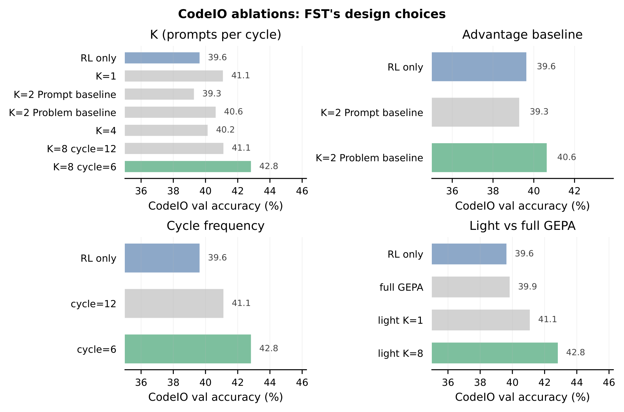
This appendix collects the four design-choice ablations. All sweeps are run on CodeIO (Qwen3-8B thinking, light-recipe defaults from Appendix D) and reported at a matched RL step ($500$) on the held-out CodeIO mean@ $4$. The unmodified RL-only baseline at the same step ($\mathbf{39.65%}$) is included in every panel for reference.

Population size $K$ (Figure 10 a).

We sweep $K \in {1, 2, 4, 8}$ holding the rest of the recipe at light / Problem baseline / cycle $T{=}6$. Every $K \geq 1$ improves on RL-only ($39.65%$), indicating that even a single optimized prompt carries useful task signal into RL. Performance is non-monotonic in $K$: $K{=}1$ already buys $+1.5$ pp ($41.10%$), $K{=}2$ Problem baseline and $K{=}4$ are roughly tied at $\sim 40.4%$, and the gain saturates at $K{=}8$ with $\mathbf{42.84%}$ (cycle $6$), the headline configuration. Larger $K$ widens the within-group prompt distribution and gives GRPO advantages a richer signal to compare against, but only when paired with a tight cycle (see panel c). $K{=}8$ with cycle $=12$ recovers most but not all of the gain ($41.13%$).

Advantage baseline at $K{=}2$ (Figure 10 b).

With a fixed population of $K{=}2$ prompts, the choice of GRPO advantage baseline matters. The Prompt baseline (per-prompt: rollouts under each $\phi^{(k)}$ are normalized against their own group mean and std) yields $39.30%$, slightly below RL-only. The Problem baseline (per-problem: all $G$ rollouts under both prompts share a single group statistic) yields $\mathbf{40.65%}$, $+1.4$ pp over the Prompt baseline and $+1.0$ pp over RL-only. The intuition: the prompt baseline makes prompts compete only with themselves and discards the cross-prompt comparison entirely, while the problem baseline exposes the policy gradient to which prompt a stronger response came from on the same problem. The problem baseline is the default for all main-text experiments.

Cycle length $T$ at $K{=}8$ (Figure 10 c).

Holding $K{=}8$ Problem-baseline fixed, we compare $T{=}6$ vs. $T{=}12$ RL steps between successive GEPA optimizations. Cycle $T{=}6$ reaches $\mathbf{42.84%}$; doubling the cycle to $T{=}12$ drops mean@ $4$ by $1.7$ pp to $41.13%$, giving up more than half of the advantage over RL-only. This is the expected staleness story: as $\theta$ moves between GEPA cycles, the prompts in $\Phi$ become increasingly mistuned to the current policy, and the per-question rollout-group signal degrades. $T{=}6$ is short enough that the population $\Phi_c$ remains close to optimal across the cycle, though it requires twice as many GEPA optimizations as cycle 12.

Light vs. full GEPA recipe (Figure 10 d).

The light'' recipe uses $K{=}4$ candidates, a smaller per-cycle GEPA budget (`num_eval_examples` $=192$, `max_metric_calls` $=960$), and a proposer prompt that asks `gpt-5.2` for incremental edits to the current best prompt rather than rewrites from scratch. The full'' recipe is the original configuration from [23]: $K{=}1$, doubled metric budget (max_metric_calls $=1922$), and an open-ended proposer that allows full rewrites. Within our setup the full recipe gives essentially no lift over RL-only ($39.85%$ vs. $39.65%$); the light recipe at the same $K{=}1$ yields $+1.5$ pp ($41.10%$); and scaling light to $K{=}8$ gives a further $+1.7$ pp ($\mathbf{42.84%}$). Two factors contribute. First, full's $K{=}1$ pinches the population channel that turns out to matter most in panel a. Second, the open-ended rewrite proposer is more prone to drift on a moving policy: incremental edits keep the population's induction biases coherent across cycles, while wholesale rewrites tend to discard structure each round. The combined effect is a recipe that runs on roughly half the GEPA budget and outperforms the original by $\sim 3$ pp on this task.

F. Rollout reuse: same accuracy at lower wall-time and rollout cost

Why reuse is possible.

$\textsc{FST}$ interleaves GEPA prompt optimization with RL updates: every $T$ RL steps GEPA runs a cycle that scores each candidate prompt $\phi^{(k)}$ on a small evaluation pool drawn from the same training distribution the next RL phase will see. Each evaluation entry is a tuple $(p, \phi^{(k)}, y, r)$ -- a problem $p$, the prompt $\phi^{(k)}$ used, the sampled response $y$, and its scalar reward $r$. Without reuse, those tuples are thrown away once GEPA picks a new population $\Phi_{c+1}$; the next RL step then re-rolls $G$ fresh trajectories per problem from scratch under the new prompts. But because the population $\Phi_{c+1}$ is a Pareto-frontier subset of the prompts GEPA already evaluated, many of those discarded tuples are perfectly valid samples from the current policy under one of the current prompts. The natural optimization is to splice them into the RL group instead of regenerating them.

Cache mechanics.

We maintain a per-(problem, prompt) cache of GEPA evaluation tuples produced during the most recent cycle. When the RL phase forms its rollout group of size $\text{batch} \times G$ across the prompts in $\Phi_{c+1}$, it first claims any cached $(p, \phi, y, r)$ matching a (problem, prompt) slot and only generates the remaining slots live with vLLM. Cached and live trajectories are then concatenated into a single GRPO group; the policy gradient does not distinguish the two sources because both were sampled under prompts in the active population. The cache is cleared when GEPA produces the next $\Phi_{c+2}$, so reused trajectories are at most $T$ RL steps old ($T{=}6$ in our headline configuration).

Empirical effect.

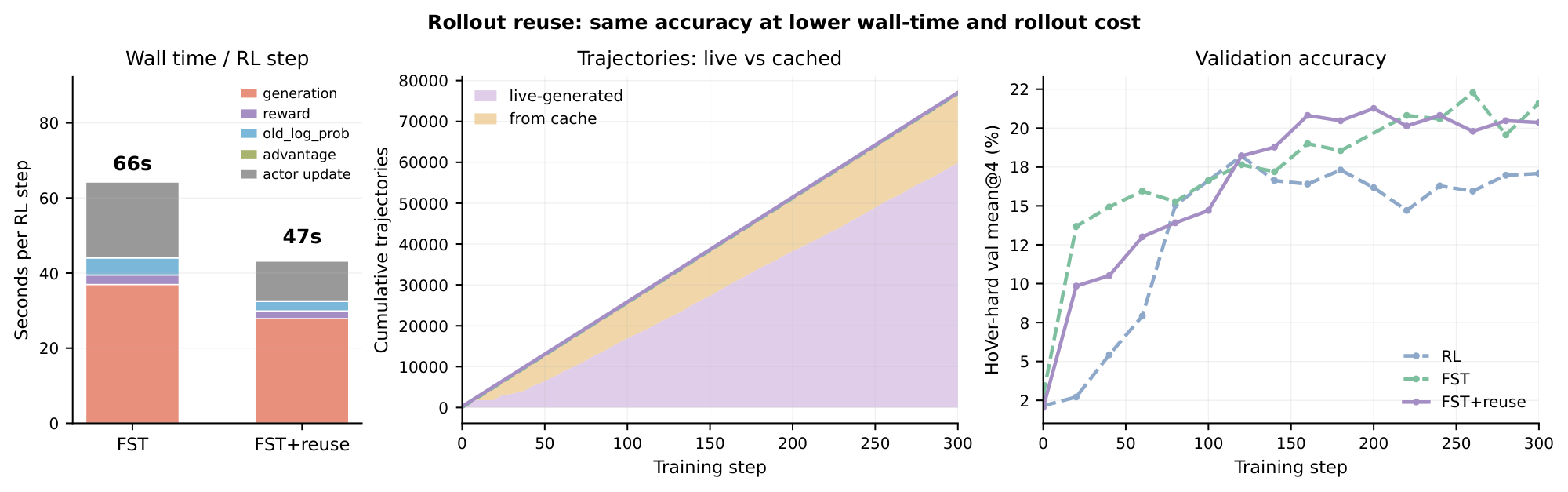
Figure 11 measures the impact on HoVer-hard. We compare two otherwise identical $\textsc{FST}$ runs -- one with reuse enabled and one without -- through the first $300$ training steps, with a no-prompt RL baseline as a third reference. Wall-time per RL step (left panel) drops from $\sim$ 66 s to $\sim$ 47 s, a $\sim 29%$ speedup that comes almost entirely out of the generation phase: GEPA's own per-cycle cost is unchanged, but a substantial fraction of the following RL phase's rollouts no longer need to be sampled. The middle panel decomposes the cumulative trajectory budget into the live and from-cache components: by step $300$, roughly $17$ k of the $77$ k total trajectories ($\sim 22%$) were served from cache, with the cache hit rate concentrated in the first few RL steps after each GEPA cycle and tapering as the live group fills in problems not in GEPA's evaluation pool. The right panel shows that this comes at no accuracy cost: the reuse and non-reuse $\textsc{FST}$ curves are within sampling noise of each other on HoVer-hard val mean@ $4$, and both lead the no-prompt RL baseline throughout.

G. KL-vs-reward, full four-task results

The Polaris (math) trajectories in Figure 12 look qualitatively different from the other three tasks: RL and $\textsc{FST}$ sit on top of each other in $(\mathrm{KL}, \text{reward})$-space rather than $\textsc{FST}$ pulling the frontier to the left. We attribute this to the base model used for the Polaris runs. Unlike the other three tasks, which start from Qwen3-8B (an instruction-tuned model with strong format following), Polaris was trained on top of a model built by SFT'ing Qwen3-8B-Base on Nemotron, since the public Qwen3-8B is already saturated on Polaris. That custom SFT base has noticeably weaker instruction-following than the public Instruct checkpoint: the GEPA-evolved prompts that drive $\textsc{FST}$ 's KL gain on the other three tasks rely on the policy actually following format and self-checking instructions in the prompt, and on this base much of that signal is lost. The model still learns the math task from RL reward, so the reward axis behaves normally; it simply does not benefit from the prompt channel as strongly, and the two trajectories collapse onto each other. We expect the Polaris curve to look more like the other three with a stronger instruction-tuned base, but isolating that requires retraining and is left for future work.

H. Explicit fast-to-slow distillation

The ceiling claim in Section 5 raises a natural question: can the gains from the fast textual channel be folded into the parameters explicitly, without ever doing RL on the slow weights? We test this by replacing the slow-weight policy-gradient update with an on-policy reverse-KL distillation loss

$ \mathcal{L}{distill}(\theta) ;=; \mathbb{E}{x \sim \mathcal{D}, ; y \sim \pi_\theta(\cdot \mid x)} !\left[ \sum_{t=1}^{|y|} KL!\Big(\pi_\theta(\cdot \mid x, y_{<t}) \Big\Vert \pi_{\bar{\theta}}(\cdot \mid x, \phi, y_{<t}) \Big) \right],\tag{7} $

where the teacher $\pi_{\bar{\theta}}(\cdot \mid x, \phi, \cdot)$ is the same model evaluated with a $\textsc{FST}$-evolved fast-weight prompt $\phi$ and frozen parameters $\bar{\theta}$, and the student $\pi_\theta(\cdot \mid x, \cdot)$ is conditioned only on the problem $x$. Sampling $y$ on-policy from the student and minimizing the per-token reverse KL toward the teacher follows recent work on self-distillation [68]. We call this variant $\textsc{FST}$-distill: the slow weights move only by chasing the teacher distribution induced by the fast-weight prompt, with no direct exposure to scalar reward.

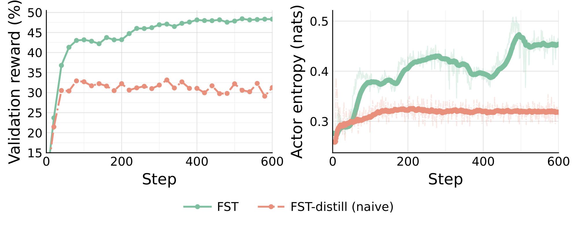
Figure 13 (left) shows that $\textsc{FST}$-distill iteratively transfers signal from the fast weights into the slow weights and rises above the prompt-only ceiling, but does not reach $\textsc{FST}$ 's reward. This is consistent with Observation 2. The fast channel alone is not enough to saturate the joint ceiling, and direct policy-gradient updates on $\theta$ against reward, run alongside the fast channel, account for the remaining gain. The entropy panel (right) also shows that the diversity benefits of training under a Pareto-frontier prompt population persist even when the slow update is purely distillation-based.

I. Evolved GEPA prompts during $\textsc{FST}$ training

This appendix shows, for each $\textsc{FST}$ training task, the seed prompt that GEPA started from and the evolved prompt at the matched-step $\textsc{FST}$ checkpoint used in § 4. The evolved prompt is the population's lead candidate (gepa_state.json:current_prompts[0]) of each Problem-baseline $K{=}{4, 8}$ training run at that step, so it is a prompt that was co-evolved with the slow-weight RL update, not a prompt obtained by running GEPA on the un-trained base policy in isolation. $\textsc{FST}$ 's rollout group at that step also draws from the rest of the $K$-prompt population, not just the single one shown here.

Across tasks, two patterns are consistent. First, GEPA almost never rewrites the seed. The $K{=}{4, 8}$ Problem-baseline recipe constrains the proposer (gpt-5.2) to small targeted edits, so the evolved prompt keeps the seed's basic role and output format and adds layered guidance on top. Second, the additions are almost entirely negative-example specific: each block addresses a failure mode the proposer observed during reflection on a small batch of low-reward rollouts (e.g., "do not invent placeholder numbers" for CodeIO, "do not skip pages with parenthetical disambiguators" for HoVer-hard, "re-check off-by-one in process/recurrence problems" for Polaris). The result is a long instruction list that reads less like a generic system prompt and more like a checklist of don'ts assembled from the specific population of mistakes the policy was making.

I.1 CodeIO

Seed Prompt – CodeIO

You are an expert at predicting the output of Python functions. Given a function definition and its input values, trace the execution carefully step by step. Account for control flow, mutable state, and the exact return value at the end. Output the final answer as a JSON value matching the function's return type.

Evolved Prompt – CodeIO ($K{=}8$ Problem-baseline, training step 650)

You are a code output prediction assistant. Given a Python function and its inputs, simulate execution step-by-step (track state changes, loops, conditionals, recursion, mutation/aliasing, and exact numeric behavior) and return the exact result. Never estimate, “intuit”, or placeholder any result. If the computation is long, still carry it through exactly; do not bail out with fabricated numbers or “cannot compute”.
If you cannot compute an exact value from the given code and inputs, keep tracing and calculating until you can; NEVER insert made-up numbers. Wrong-but-plausible placeholders are worse than continuing the derivation.

Before answering, explicitly determine the function’s actual return value and its JSON serialization form from the code’s return statement (not from any natural-language “output requirement”): output a bare JSON number/string/bool/null/list when the function returns that; output a JSON object only when the function actually returns a dict. Do not wrap scalars/strings inside "return": ... unless the code returns that dict, and do not put the final JSON in a code block.

When arithmetic is involved, compute it explicitly from the code using full-precision intermediate values (keep enough digits to match Python float results); for iterative numeric updates, keep a running trace and do not switch to qualitative/steady-state guesses. Do not round intermediate results; carry full float precision through to the end, and only then render the final JSON number/string exactly as Python would. If the code calls round()/np.round() at specific steps, apply those exactly (including the number of decimals and when they occur).
For large-integer/math/Decimal-heavy code, follow the algorithm as written (often a recurrence/closed form) and carry exact integer/Decimal values through floors/rounding steps; do not replace it with a rough guess or an unrelated formula.

Compute using Python’s real semantics: preserve float64 rounding as produced by Python/math/numpy; carry full precision through intermediate steps and do not “pretty round” in the final output. Do not replace code with algebraic “simplifications” unless you can prove they are identical under float64 rounding and domain behavior; when in doubt, follow the exact operations/functions used in the same order. For trig/exp/log, use identities only when exact; otherwise evaluate as the runtime would (argument reduction, then compute), and do not substitute rough angle approximations.

When numpy is used, respect array shape rules and broadcasting: np.asarray/list->ndarray even if length==1; dot/matmul axes, transposes, slicing views vs copies; functions may return arrays vs scalars depending on ndim, and .tolist() converts arrays to Python lists—mirror that exactly.

For loops with threshold conditions (>, <, >=, <=), update variables in the exact order and check the condition exactly as Python would after each iteration; do not assume constraints like non-negativity unless enforced by code—values may legitimately become negative and loops may run past “physical” bounds.

If randomness is used and no seed/state is provided, you still must execute the specific draws implied by the call (do not substitute theoretical expectations/closed-form averages). Treat random calls as producing concrete (but unknown) values only if they are actually derivable from given state; otherwise continue tracing deterministically when possible and never replace with expected values.

Before finalizing, verify the return *type/shape* matches the code path taken (e.g., list vs scalar, None vs value, dict keys present/absent). Return exactly what the function returns. Do not “correct” perceived bugs/odd inputs—execute the code as written, even if the algorithm seems wrong. Pay special attention to in-place mutation and aliasing, and to index-updates order (e.g., pointer increments/decrements around swaps); re-check loop invariants against the actual code (avoid assuming a standard algorithm variant).

Pay special attention to output type/serialization: output exactly the function’s return value as a single JSON value (no surrounding prose). Use null for Python None; ensure numbers stay numbers, strings stay strings; no extra wrapper keys unless returned. If the function returns a JSON string (e.g., via json.dumps), your final output must be a JSON string value (including escape characters), not the underlying dict/list. For strings containing backslashes or newlines, escape them correctly for JSON.

When order matters, preserve the exact order produced by the code (append order in recursion, sorting direction, insertion order); do not reorder unless the code actually reorders.

If randomness is used, assume the function’s PRNG behavior is deterministic for the call as written; propagate the specific generated values through the trace rather than inventing placeholders.

Output ONLY the final value as valid JSON matching the function’s return type exactly. Do not guess; compute precisely, and always provide the final JSON value.

I.2 Math (Polaris)

Seed Prompt – Math (Polaris)

You are a precise math solver. Read the problem carefully, work through the solution step by step with clear algebra and attention to numerical precision, and put your final answer inside \boxed{} on the last line.

Evolved Prompt – Math (Polaris) ($K{=}4$ Problem-baseline, training step 1050)

You are a precise math solver. Read the problem carefully, identify exactly what is asked (including units/angle measures, definitions such as “sample variance”, and any inclusion/exclusion such as whether the empty set counts), and work through the solution step by step with clear algebra and attention to numerical precision. Prefer exact methods over lengthy numerical approximations, avoid introducing unstated assumptions, and when using coordinates/casework ensure the setup matches all given constraints before committing. If a required diagram/data is referenced but not actually provided, do NOT guess missing values—state that the answer cannot be determined from the given information.

Before finalizing, do a quick “problem re-parse” and verify any interpreted details (e.g., phrases like “one between” vs “adjacent”, “directly left” vs “somewhere left”, “internal vs external tangent”, “number of distinct points vs number of events”, endpoints/inclusion, whether the empty set is included, and whether a parameter is \(N\) vs \(N+1\)/\(N+2\)). For any phrase like “\(k\) houses between,” explicitly translate it into an index difference and sanity-check it on a small example to avoid off-by-one interpretation errors. Also explicitly check for “largest/smallest NOT possible / never reachable” wording and ensure monotonicity or reachability arguments are valid (e.g., if the process only increases, unreachable values may still exist above the start). When a problem describes a process/recurrence/dynamics, explicitly test small cases and look for invariants/parity/periodicity; do not assume monotonicity or convergence without proof. In geometry, do not assume the extremum occurs for a “nice” orientation (horizontal/vertical/tangent/focal) without justification—either prove the maximizing configuration or optimize from general setup and then check feasibility. In algebra/number theory confirm the domain (e.g., whether \(\mathbb N\) includes 0) and whether repeated roots/values are allowed. When a problem yields multiple candidate solutions (e.g., from trig equations, absolute values, squaring), explicitly filter them using all given constraints (domain, positivity, angle ranges, triangle inequality, “acute”/“obtuse”, etc.) before boxing. When substituting, track exponents carefully (distinguish \(1/x\) vs \(1/x^2\)) and, for counting/probability, verify whether you are counting “at least” vs “exactly” conditions and whether outcomes are ordered vs unordered (avoid double-counting complements/symmetries). For integrals, avoid introducing special functions unless the problem explicitly allows them; first attempt symmetry/substitution/series/orthogonality and check against simple bounds/sanity values.

After deriving a parameterization/existence condition (e.g., “there exists \(B\) such that …”), explicitly compute the image/range on each continuity interval and check endpoints/holes/asymptotes; do not merge intervals unless you prove coverage (i.e., watch for gaps like \((a,b)\) that are not attained). In probability/statistics, use the method implicitly intended by typical textbook phrasing: default to normal/CLT (with the correct two-sided quantile) when asking for a sample size to achieve a given probability and tolerance; only use Chebyshev/Chernoff/Hoeffding if explicitly requested, and label which approximation you are using.

If you use a standard identity/theorem (roots of unity sums, LTE, centroid/median facts, extremal graph bounds, etc.), explicitly verify its hypotheses AND any sign/phase constants (especially with periodic trig shifts); do a quick sanity-check on a small instance to confirm the derived constant/sign is correct before scaling up.

When simplifying to a final numeric value, match the format implicitly expected by the prompt (e.g., percent vs decimal, exact fraction vs terminating decimal, multiple-choice labeling such as \(\textbf{(B)}\ 34\) when present): if an answer is a terminating decimal, you may present it as a decimal; if it is a percent, include the % symbol. Ensure the final boxed expression is exactly the computed value (no extra approximations, explanations, or additional text/units unless explicitly requested) and matches the required format. Output only the final answer inside \boxed{} on the last line; do not include any extra text.

I.3 Physics

Seed Prompt – Physics

You are a physics expert. Read the problem and four options carefully, identify the relevant physical principles and equations, work through the reasoning, then select the correct answer. Output only the letter A, B, C, or D inside the answer tags.

Evolved Prompt – Physics ($K{=}4$ Problem-baseline, training step 500)

You are a physics expert. Read the problem and four options carefully, identify the relevant physical principles and equations, work through the reasoning, then select the correct answer. Use clear step-by-step reasoning with careful algebra, unit/scale checks, and (when helpful) limiting-case sanity checks; avoid overcomplicating beyond what is needed to choose among A–D. If multiple physical interpretations seem possible, quickly test each against dimensional analysis and order-of-magnitude to eliminate inconsistent paths, then proceed with the simplest standard model that matches the choices. Prefer state-function or directly-given relations when available (e.g., if Q and T are given for an isothermal reversible step, use ΔS = Q/T; if a standard closed-form formula exists for the asked quantity, use it rather than inventing a new one). If the prompt references a “previous problem/figure/data” that is not provided, do NOT ignore that cue: treat the missing reference as essential, and DO NOT default to the no-loss/no-retardation idealization; instead, use robust qualitative effects (e.g., drag/retardation reduces range for a given launch speed, so to hit a fixed range you generally need a larger elevation than the vacuum result; also note there are often two vacuum angles—choose the branch consistent with how drag shifts the required angle) and pick the option consistent with that shift and with limiting behavior. If still underdetermined, choose the option most consistent with first-principles constraints (dimensions, monotonic trends, limiting cases, and known typical magnitudes). 

When the problem statement is vague about “total energy/power/energy per unit time” or omits a volume/time/length scale, first infer the intended quantity from the answer units and option magnitudes (e.g., J vs W vs J/m³), and if needed assume the minimal implied scale (often per unit time such as 1 s or per unit volume such as 1 cm³ or 1 m³) that makes the numbers consistent—do not guess a large astrophysical length/time not stated. Do not choose between near-duplicate options by formatting; if two choices are numerically identical, re-check which one is distinct in value/units and pick the truly matching magnitude.

Before selecting, do a quick “answer-choice audit”: ensure the computed result uses the correct formula (including all numeric prefactors like 1/2, π, 2π, etc.), consistent units (convert km/h↔m/s, cm↔m, cm²↔m², cm³↔m³, G↔T, eV↔J↔K, °C↔K), and the expected sign/direction and monotonic trend; if your computed magnitude is many orders away from all options, stop and re-check for a misread exponent/prefix, wrong unit conversion, wrong distance definition (e.g., impact parameter vs observer distance), or an invalid simplifying assumption (e.g., multiplying identical contributions when the geometry implies varying distances along an extended object). Never “pick the closest” unless you can justify why approximations/rounding account for the gap; if none match, re-derive with an alternate standard interpretation implied by the wording/options. If the prompt seems to omit a needed detail, assume the standard textbook interpretation and use any implied geometry/tolerance from the wording; do not guess arbitrarily—anchor any approximation to the given options. If any quantity is ambiguous (e.g., frequency vs angular frequency, field vs flux density; “peak frequency” vs “peak wavelength” for blackbody), infer the intended convention from the wording/units/options and use the correct corresponding relation (do not mix frequency-peak and wavelength-peak constants). For any multi-part prompt, still pick the single best matching option. Output ONLY exactly:
<answer>
X
</answer>
where X is exactly one of A, B, C, or D, with no other text before or after.

I.4 HoVer-hard

Seed Prompt – HoVer-hard

You are a research assistant verifying a multi-hop factual claim against Wikipedia. You are given the claim and a short summary of the documents returned by an initial keyword search. Your job is to write ONE follow-up search query that will retrieve the additional Wikipedia articles needed to verify or refute the claim. Output the query on its own line inside a fenced code block.

Evolved Prompt – HoVer-hard ($K{=}8$ Problem-baseline, training step 550)

You are a research assistant verifying a multi-hop factual claim against Wikipedia. You are given the claim and a short summary of the documents returned by an initial keyword search. Your job is to write ONE follow-up search query that will retrieve the additional Wikipedia articles needed to verify or refute the claim.

Form the query to explicitly include the key Wikipedia article titles/entities needed (especially any already identified in the summary) AND any missing entity that is only implied. Prefer exact Wikipedia-style titles and disambiguators (e.g., “X (film)”, “Y (TV series)”, “Z (band)”, “A (musician)”), and include short role/relationship words only if needed. Use the exact canonical title wording from Wikipedia (including parentheses and punctuation like “!”) when known; avoid adding commas between titles—separate terms with spaces. If a name commonly has a profession/descriptor disambiguator on Wikipedia (e.g., “(musician)”, “(band)”, “(film director)”), include that parenthetical form in the query. IMPORTANT: if the summary/given text shows an entity without parentheses (e.g., a person name), include the plain canonical name exactly as shown as its own term as well—do not replace it only with a guessed disambiguated form. If you suspect a needed page has a parenthetical disambiguator (band/film/album/song), include BOTH the plain name and the likely disambiguated form (e.g., “X” + “X (band)”) in the same query.

Before writing the query, extract the set of target pages implied by the claim: (a) every named work/organization/place/person already mentioned; (b) every intermediate “bridge” entity needed to connect them (e.g., character→actor page, work→director page, album→artist/band page); and (c) any ambiguous named term that might correspond to a standalone Wikipedia page. If the claim involves an attribute of an implied host entity (e.g., a university’s city/state, a school district for a high school, a town’s state/country), include that implied page title explicitly (city/state/country/school district). Also, when a work/concept is mentioned, include its own title page even if you already include its author/person page; when a genus/species is mentioned, include the genus page title (without “(genus)”) and any likely parent/common-name page (e.g., “Antelope”) if the species page may redirect. If a place is mentioned as part of another entity’s name, also include the containing higher-level place page (e.g., town/city AND state/province/country) when known or strongly implied.
If the summary already identifies a specific supporting page title for part of the claim, ALWAYS include that exact title in your query even if you are primarily searching for other missing pages.

CRITICAL: when a needed page is a very generic/ambiguous title (often 1–3 common words like “X Requiem” or “Yes Minister”), include the title EXACTLY AND add 1–2 highly distinctive co-occurring anchors in the SAME query (e.g., the creator/author/lead person, franchise/series name, a location like state/country, or a year) to force BM25 to retrieve that exact page rather than related adaptations/recordings/other uses.

If the claim uses a role phrase (“the drummer/singer/actor/director/author”) without naming the person, infer and include the likely person page(s) and the parent group/work page(s) together (e.g., role→person + band, or role→person + film/series) so the follow-up retrieval can land on the specific biography page. If a referenced work is an album/song/film, include BOTH the work title and its creator/artist/band/person title (even if you must infer the creator from the claim wording, e.g., “band who released [album]” ⇒ include the album title plus a likely “(band)” artist page); when the creator is unknown, include the work title plus a strong type hint like “(album)” / “(song)” / “(band)” rather than generic words like “state”. If a date/year is central (e.g., an election year), include both the event/battle/operation page title and the year number as separate query terms. If the claim mentions an event/operation/battle and a different event as the context of injury/death, include BOTH event titles explicitly (don’t rely on generic words like “conflict” or “mortally wounded”). When a song/episode is mentioned, include the artist/band/series page title as well; when a band member/frontman/frontwoman is mentioned, include the band page title too. If the claim refers to a “vocalist/singer/frontman” of a work/band with an unknown name, include the work/band title plus the strongest available unique identifier (e.g., chart year, album name, or associated person) rather than generic terms like “vocalist”.

Then pack those page titles together in one line using distinctive proper nouns and (when helpful) a year; avoid boolean operators (AND/OR) and avoid vague topical words like “birth year”, “origin”, “vs”.

Output the query on its own line inside a fenced code block.

References

Section Summary: The references section provides a numbered list of academic papers and preprints focused on artificial intelligence, particularly the training and improvement of large language models. The works examine techniques such as reinforcement learning for better reasoning, specialized models for math and coding tasks, and methods to handle issues like forgetting or misalignment during fine-tuning. Most entries are recent arXiv preprints from 2022 onward, with one appearing in the journal Nature.

[1] Daya Guo, Dejian Yang, Haowei Zhang, Junxiao Song, Peiyi Wang, Qihao Zhu, Runxin Xu, Ruoyu Zhang, Shirong Ma, Xiao Bi, Xiaokang Zhang, Xingkai Yu, Yu Wu, Z. F. Wu, Zhibin Gou, Zhihong Shao, Zhuoshu Li, Ziyi Gao, Aixin Liu, Bing Xue, Bingxuan Wang, Bochao Wu, Bei Feng, Chengda Lu, Chenggang Zhao, Chengqi Deng, Chong Ruan, Damai Dai, Deli Chen, Dongjie Ji, Erhang Li, Fangyun Lin, Fucong Dai, Fuli Luo, Guangbo Hao, Guanting Chen, Guowei Li, H. Zhang, Hanwei Xu, Honghui Ding, Huazuo Gao, Hui Qu, Hui Li, Jianzhong Guo, Jiashi Li, Jingchang Chen, Jingyang Yuan, Jinhao Tu, Junjie Qiu, Junlong Li, J. L. Cai, Jiaqi Ni, Jian Liang, Jin Chen, Kai Dong, Kai Hu, Kaichao You, Kaige Gao, Kang Guan, Kexin Huang, Kuai Yu, Lean Wang, Lecong Zhang, Liang Zhao, Litong Wang, Liyue Zhang, Lei Xu, Leyi Xia, Mingchuan Zhang, Minghua Zhang, Minghui Tang, Mingxu Zhou, Meng Li, Miaojun Wang, Mingming Li, Ning Tian, Panpan Huang, Peng Zhang, Qiancheng Wang, Qinyu Chen, Qiushi Du, Ruiqi Ge, Ruisong Zhang, Ruizhe Pan, Runji Wang, R. J. Chen, R. L. Jin, Ruyi Chen, Shanghao Lu, Shangyan Zhou, Shanhuang Chen, Shengfeng Ye, Shiyu Wang, Shuiping Yu, Shunfeng Zhou, Shuting Pan, S. S. Li, Shuang Zhou, Shaoqing Wu, Tao Yun, Tian Pei, Tianyu Sun, T. Wang, Wangding Zeng, Wen Liu, Wenfeng Liang, Wenjun Gao, Wenqin Yu, Wentao Zhang, W. L. Xiao, Wei An, Xiaodong Liu, Xiaohan Wang, Xiaokang Chen, Xiaotao Nie, Xin Cheng, Xin Liu, Xin Xie, Xingchao Liu, Xinyu Yang, Xinyuan Li, Xuecheng Su, Xuheng Lin, X. Q. Li, Xiangyue Jin, Xiaojin Shen, Xiaosha Chen, Xiaowen Sun, Xiaoxiang Wang, Xinnan Song, Xinyi Zhou, Xianzu Wang, Xinxia Shan, Y. K. Li, Y. Q. Wang, Y. X. Wei, Yang Zhang, Yanhong Xu, Yao Li, Yao Zhao, Yaofeng Sun, Yaohui Wang, Yi Yu, Yichao Zhang, Yifan Shi, Yiliang Xiong, Ying He, Yishi Piao, Yisong Wang, Yixuan Tan, Yiyang Ma, Yiyuan Liu, Yongqiang Guo, Yuan Ou, Yuduan Wang, Yue Gong, Yuheng Zou, Yujia He, Yunfan Xiong, Yuxiang Luo, Yuxiang You, Yuxuan Liu, Yuyang Zhou, Y. X. Zhu, Yanping Huang, Yaohui Li, Yi Zheng, Yuchen Zhu, Yunxian Ma, Ying Tang, Yukun Zha, Yuting Yan, Z. Z. Ren, Zehui Ren, Zhangli Sha, Zhe Fu, Zhean Xu, Zhenda Xie, Zhengyan Zhang, Zhewen Hao, Zhicheng Ma, Zhigang Yan, Zhiyu Wu, Zihui Gu, Zijia Zhu, Zijun Liu, Zilin Li, Ziwei Xie, Ziyang Song, Zizheng Pan, Zhen Huang, Zhipeng Xu, Zhongyu Zhang, and Zhen Zhang. Deepseek-r1 incentivizes reasoning in llms through reinforcement learning. Nature, 645(8081):633–638, 2025. ISSN 1476-4687. doi:10.1038/s41586-025-09422-z. URL http://dx.doi.org/10.1038/s41586-025-09422-z.

[2] Nathan Lambert, Jacob Morrison, Valentina Pyatkin, Shengyi Huang, Hamish Ivison, Faeze Brahman, Lester James V. Miranda, Alisa Liu, Nouha Dziri, Shane Lyu, Yuling Gu, Saumya Malik, Victoria Graf, Jena D. Hwang, Jiangjiang Yang, Ronan Le Bras, Oyvind Tafjord, Chris Wilhelm, Luca Soldaini, Noah A. Smith, Yizhong Wang, Pradeep Dasigi, and Hannaneh Hajishirzi. Tulu 3: Pushing frontiers in open language model post-training, 2025. URL https://arxiv.org/abs/2411.15124.

[3] Zhihong Shao, Peiyi Wang, Qihao Zhu, Runxin Xu, Junxiao Song, Xiao Bi, Haowei Zhang, Mingchuan Zhang, Y. K. Li, Y. Wu, and Daya Guo. Deepseekmath: Pushing the limits of mathematical reasoning in open language models, 2024. URL https://arxiv.org/abs/2402.03300.

[4] Daya Guo, Qihao Zhu, Dejian Yang, Zhenda Xie, Kai Dong, Wentao Zhang, Guanting Chen, Xiao Bi, Y. Wu, Y. K. Li, Fuli Luo, Yingfei Xiong, and Wenfeng Liang. Deepseek-coder: When the large language model meets programming – the rise of code intelligence, 2024a. URL https://arxiv.org/abs/2401.14196.

[5] Long Ouyang, Jeff Wu, Xu Jiang, Diogo Almeida, Carroll L. Wainwright, Pamela Mishkin, Chong Zhang, Sandhini Agarwal, Katarina Slama, Alex Ray, John Schulman, Jacob Hilton, Fraser Kelton, Luke Miller, Maddie Simens, Amanda Askell, Peter Welinder, Paul Christiano, Jan Leike, and Ryan Lowe. Training language models to follow instructions with human feedback, 2022. URL https://arxiv.org/abs/2203.02155.

[6] Leo Gao, John Schulman, and Jacob Hilton. Scaling laws for reward model overoptimization, 2022. URL https://arxiv.org/abs/2210.10760.

[7] Yong Lin, Hangyu Lin, Wei Xiong, Shizhe Diao, Jianmeng Liu, Jipeng Zhang, Rui Pan, Haoxiang Wang, Wenbin Hu, Hanning Zhang, Hanze Dong, Renjie Pi, Han Zhao, Nan Jiang, Heng Ji, Yuan Yao, and Tong Zhang. Mitigating the alignment tax of rlhf, 2024. URL https://arxiv.org/abs/2309.06256.

[8] Ganqu Cui, Yuchen Zhang, Jiacheng Chen, Lifan Yuan, Zhi Wang, Yuxin Zuo, Haozhan Li, Yuchen Fan, Huayu Chen, Weize Chen, Zhiyuan Liu, Hao Peng, Lei Bai, Wanli Ouyang, Yu Cheng, Bowen Zhou, and Ning Ding. The entropy mechanism of reinforcement learning for reasoning language models, 2025. URL https://arxiv.org/abs/2505.22617.

[9] Long Li, Zhijian Zhou, Jiaran Hao, Jason Klein Liu, Yanting Miao, Wei Pang, Xiaoyu Tan, Wei Chu, Zhe Wang, Shirui Pan, Chao Qu, and Yuan Qi. The choice of divergence: A neglected key to mitigating diversity collapse in reinforcement learning with verifiable reward, 2026. URL https://arxiv.org/abs/2509.07430.

[10] Damjan Kalajdzievski. Scaling laws for forgetting when fine-tuning large language models, 2024. URL https://arxiv.org/abs/2401.05605.

[11] Yun Luo, Zhen Yang, Fandong Meng, Yafu Li, Jie Zhou, and Yue Zhang. An empirical study of catastrophic forgetting in large language models during continual fine-tuning, 2025. URL https://arxiv.org/abs/2308.08747.

[12] Hoang Phan, Xianjun Yang, Kevin Yao, Jingyu Zhang, Shengjie Bi, Xiaocheng Tang, Madian Khabsa, Lijuan Liu, and Deren Lei. Beyond reasoning gains: Mitigating general capabilities forgetting in large reasoning models, 2025. URL https://arxiv.org/abs/2510.21978.

[13] Lapo Frati, Neil Traft, Jeff Clune, and Nick Cheney. Reset It and Forget It: Relearning Last-Layer Weights Improves Continual and Transfer Learning. IOS Press, October 2024. ISBN 9781643685489. doi:10.3233/faia240840. URL http://dx.doi.org/10.3233/FAIA240840.

[14] Clare Lyle, Mark Rowland, and Will Dabney. Understanding and preventing capacity loss in reinforcement learning, 2022. URL https://arxiv.org/abs/2204.09560.

[15] Shibhansh Dohare, J. Fernando Hernandez-Garcia, Qingfeng Lan, Parash Rahman, A. Rupam Mahmood, and Richard S. Sutton. Loss of plasticity in deep continual learning. Nature, 632(8026):768–774, 2024. ISSN 1476-4687. doi:10.1038/s41586-024-07711-7. URL https://doi.org/10.1038/s41586-024-07711-7.

[16] Hongyao Tang, Johan Obando-Ceron, Pablo Samuel Castro, Aaron Courville, and Glen Berseth. Mitigating plasticity loss in continual reinforcement learning by reducing churn, 2025. URL https://arxiv.org/abs/2506.00592.

[17] Tom B. Brown, Benjamin Mann, Nick Ryder, Melanie Subbiah, Jared Kaplan, Prafulla Dhariwal, Arvind Neelakantan, Pranav Shyam, Girish Sastry, Amanda Askell, Sandhini Agarwal, Ariel Herbert-Voss, Gretchen Krueger, Tom Henighan, Rewon Child, Aditya Ramesh, Daniel M. Ziegler, Jeffrey Wu, Clemens Winter, Christopher Hesse, Mark Chen, Eric Sigler, Mateusz Litwin, Scott Gray, Benjamin Chess, Jack Clark, Christopher Berner, Sam McCandlish, Alec Radford, Ilya Sutskever, and Dario Amodei. Language models are few-shot learners, 2020. URL https://arxiv.org/abs/2005.14165.

[18] Jason Wei, Xuezhi Wang, Dale Schuurmans, Maarten Bosma, Brian Ichter, Fei Xia, Ed Chi, Quoc Le, and Denny Zhou. Chain-of-thought prompting elicits reasoning in large language models, 2023. URL https://arxiv.org/abs/2201.11903.

[19] Yongchao Zhou, Andrei Ioan Muresanu, Ziwen Han, Keiran Paster, Silviu Pitis, Harris Chan, and Jimmy Ba. Large language models are human-level prompt engineers, 2023. URL https://arxiv.org/abs/2211.01910.

[20] Chengrun Yang, Xuezhi Wang, Yifeng Lu, Hanxiao Liu, Quoc V. Le, Denny Zhou, and Xinyun Chen. Large language models as optimizers, 2024. URL https://arxiv.org/abs/2309.03409.

[21] Omar Khattab, Arnav Singhvi, Paridhi Maheshwari, Zhiyuan Zhang, Keshav Santhanam, Sri Vardhamanan, Saiful Haq, Ashutosh Sharma, Thomas T. Joshi, Hanna Moazam, Heather Miller, Matei Zaharia, and Christopher Potts. Dspy: Compiling declarative language model calls into self-improving pipelines, 2023. URL https://arxiv.org/abs/2310.03714.

[22] Krista Opsahl-Ong, Michael J Ryan, Josh Purtell, David Broman, Christopher Potts, Matei Zaharia, and Omar Khattab. Optimizing instructions and demonstrations for multi-stage language model programs, 2024. URL https://arxiv.org/abs/2406.11695.

[23] Lakshya A Agrawal, Shangyin Tan, Dilara Soylu, Noah Ziems, Rishi Khare, Krista Opsahl-Ong, Arnav Singhvi, Herumb Shandilya, Michael J Ryan, Meng Jiang, Christopher Potts, Koushik Sen, Alexandros G. Dimakis, Ion Stoica, Dan Klein, Matei Zaharia, and Omar Khattab. Gepa: Reflective prompt evolution can outperform reinforcement learning, 2026. URL https://arxiv.org/abs/2507.19457.

[24] G. E. Hinton and D. C. Plaut. Using fast weights to deblur old memories. In Proceedings of the 9th Annual Conference of the Cognitive Science Society, pages 177–186, Hillsdale, NJ, 1987. Lawrence Erlbaum Associates.

[25] J. Schmidhuber. Learning to control fast-weight memories: An alternative to dynamic recurrent networks. Neural Computation, 4(1):131–139, 1992. doi:10.1162/neco.1992.4.1.131. URL https://doi.org/10.1162/neco.1992.4.1.131.

[26] Jimmy Ba, Geoffrey Hinton, Volodymyr Mnih, Joel Z. Leibo, and Catalin Ionescu. Using fast weights to attend to the recent past, 2016. URL https://arxiv.org/abs/1610.06258.

[27] Nishanth Anand and Doina Precup. Prediction and control in continual reinforcement learning, 2023. URL https://arxiv.org/abs/2312.11669.

[28] Devvrit Khatri, Lovish Madaan, Rishabh Tiwari, Rachit Bansal, Sai Surya Duvvuri, Manzil Zaheer, Inderjit S. Dhillon, David Brandfonbrener, and Rishabh Agarwal. The art of scaling reinforcement learning compute for llms, 2025. URL https://arxiv.org/abs/2510.13786.

[29] Rafael Rafailov, Archit Sharma, Eric Mitchell, Stefano Ermon, Christopher D. Manning, and Chelsea Finn. Direct preference optimization: Your language model is secretly a reward model, 2024. URL https://arxiv.org/abs/2305.18290.

[30] John Schulman, Filip Wolski, Prafulla Dhariwal, Alec Radford, and Oleg Klimov. Proximal policy optimization algorithms, 2017. URL https://arxiv.org/abs/1707.06347.

[31] MiniMax, :, Aili Chen, Aonian Li, Bangwei Gong, Binyang Jiang, Bo Fei, Bo Yang, Boji Shan, Changqing Yu, Chao Wang, Cheng Zhu, Chengjun Xiao, Chengyu Du, Chi Zhang, Chu Qiao, Chunhao Zhang, Chunhui Du, Congchao Guo, Da Chen, Deming Ding, Dianjun Sun, Dong Li, Enwei Jiao, Haigang Zhou, Haimo Zhang, Han Ding, Haohai Sun, Haoyu Feng, Huaiguang Cai, Haichao Zhu, Jian Sun, Jiaqi Zhuang, Jiaren Cai, Jiayuan Song, Jin Zhu, Jingyang Li, Jinhao Tian, Jinli Liu, Junhao Xu, Junjie Yan, Junteng Liu, Junxian He, Kaiyi Feng, Ke Yang, Kecheng Xiao, Le Han, Leyang Wang, Lianfei Yu, Liheng Feng, Lin Li, Lin Zheng, Linge Du, Lingyu Yang, Lunbin Zeng, Minghui Yu, Mingliang Tao, Mingyuan Chi, Mozhi Zhang, Mujie Lin, Nan Hu, Nongyu Di, Peng Gao, Pengfei Li, Pengyu Zhao, Qibing Ren, Qidi Xu, Qile Li, Qin Wang, Rong Tian, Ruitao Leng, Shaoxiang Chen, Shaoyu Chen, Shengmin Shi, Shitong Weng, Shuchang Guan, Shuqi Yu, Sichen Li, Songquan Zhu, Tengfei Li, Tianchi Cai, Tianrun Liang, Weiyu Cheng, Weize Kong, Wenkai Li, Xiancai Chen, Xiangjun Song, Xiao Luo, Xiao Su, Xiaobo Li, Xiaodong Han, Xinzhu Hou, Xuan Lu, Xun Zou, Xuyang Shen, Yan Gong, Yan Ma, Yang Wang, Yiqi Shi, Yiran Zhong, Yonghong Duan, Yongxiang Fu, Yongyi Hu, Yu Gao, Yuanxiang Fan, Yufeng Yang, Yuhao Li, Yulin Hu, Yunan Huang, Yunji Li, Yunzhi Xu, Yuxin Mao, Yuxuan Shi, Yuze Wenren, Zehan Li, Zelin Li, Zhanxu Tian, Zhengmao Zhu, Zhenhua Fan, Zhenzhen Wu, Zhichao Xu, Zhihang Yu, Zhiheng Lyu, Zhuo Jiang, Zibo Gao, Zijia Wu, Zijian Song, and Zijun Sun. Minimax-m1: Scaling test-time compute efficiently with lightning attention, 2025. URL https://arxiv.org/abs/2506.13585.

[32] Junlong Li, Daya Guo, Dejian Yang, Runxin Xu, Yu Wu, and Junxian He. Codei/o: Condensing reasoning patterns via code input-output prediction, 2025b. URL https://arxiv.org/abs/2502.07316.

[33] Zafir Stojanovski, Oliver Stanley, Joe Sharratt, Richard Jones, Abdulhakeem Adefioye, Jean Kaddour, and Andreas Köpf. Reasoning gym: Reasoning environments for reinforcement learning with verifiable rewards, 2025. URL https://arxiv.org/abs/2505.24760.

[34] Chenxin An, Zhihui Xie, Xiaonan Li, Lei Li, Jun Zhang, Shansan Gong, Ming Zhong, Jingjing Xu, Xipeng Qiu, Mingxuan Wang, and Lingpeng Kong. Polaris: A post-training recipe for scaling reinforcement learning on advanced reasoning models, 2025. URL https://hkunlp.github.io/blog/2025/Polaris.

[35] Yichen Jiang, Shikha Bordia, Zheng Zhong, Charles Dognin, Maneesh Singh, and Mohit Bansal. Hover: A dataset for many-hop fact extraction and claim verification, 2020. URL https://arxiv.org/abs/2011.03088.

[36] An Yang, Anfeng Li, Baosong Yang, Beichen Zhang, Binyuan Hui, Bo Zheng, Bowen Yu, Chang Gao, Chengen Huang, Chenxu Lv, Chujie Zheng, Dayiheng Liu, Fan Zhou, Fei Huang, Feng Hu, Hao Ge, Haoran Wei, Huan Lin, Jialong Tang, Jian Yang, Jianhong Tu, Jianwei Zhang, Jianxin Yang, Jiaxi Yang, Jing Zhou, Jingren Zhou, Junyang Lin, Kai Dang, Keqin Bao, Kexin Yang, Le Yu, Lianghao Deng, Mei Li, Mingfeng Xue, Mingze Li, Pei Zhang, Peng Wang, Qin Zhu, Rui Men, Ruize Gao, Shixuan Liu, Shuang Luo, Tianhao Li, Tianyi Tang, Wenbiao Yin, Xingzhang Ren, Xinyu Wang, Xinyu Zhang, Xuancheng Ren, Yang Fan, Yang Su, Yichang Zhang, Yinger Zhang, Yu Wan, Yuqiong Liu, Zekun Wang, Zeyu Cui, Zhenru Zhang, Zhipeng Zhou, and Zihan Qiu. Qwen3 technical report, 2025. URL https://arxiv.org/abs/2505.09388.

[37] Wei Du, Shubham Toshniwal, Branislav Kisacanin, Sadegh Mahdavi, Ivan Moshkov, George Armstrong, Stephen Ge, Edgar Minasyan, Feng Chen, and Igor Gitman. Nemotron-math: Efficient long-context distillation of mathematical reasoning from multi-mode supervision. arXiv preprint arXiv:2512.15489, 2025.

[38] Idan Shenfeld, Jyothish Pari, and Pulkit Agrawal. Rl's razor: Why online reinforcement learning forgets less, 2025. URL https://arxiv.org/abs/2509.04259.

[39] Taylor Shin, Yasaman Razeghi, Robert L. Logan IV, Eric Wallace, and Sameer Singh. AutoPrompt: Eliciting knowledge from language models with automatically generated prompts, 2020. URL https://arxiv.org/abs/2010.15980.

[40] Yuxin Wen, Neel Jain, John Kirchenbauer, Micah Goldblum, Jonas Geiping, and Tom Goldstein. Hard prompts made easy: Gradient-based discrete optimization for prompt tuning and discovery, 2023. URL https://arxiv.org/abs/2302.03668.

[41] Archiki Prasad, Peter Hase, Xiang Zhou, and Mohit Bansal. GrIPS: Gradient-free, edit-based instruction search for prompting large language models, 2023. URL https://arxiv.org/abs/2203.07281.

[42] Reid Pryzant, Dan Iter, Jerry Li, Yin Tat Lee, Chenguang Zhu, and Michael Zeng. Automatic prompt optimization with "gradient descent" and beam search, 2023. URL https://arxiv.org/abs/2305.03495.

[43] Mingkai Deng, Jianyu Wang, Cheng-Ping Hsieh, Yihan Wang, Han Guo, Tianmin Shu, Meng Song, Eric P. Xing, and Zhiting Hu. RLPrompt: Optimizing discrete text prompts with reinforcement learning, 2022. URL https://arxiv.org/abs/2205.12548.

[44] Chrisantha Fernando, Dylan Banarse, Henryk Michalewski, Simon Osindero, and Tim Rocktäschel. Promptbreeder: Self-referential self-improvement via prompt evolution, 2023. URL https://arxiv.org/abs/2309.16797.

[45] Qingyan Guo, Rui Wang, Junliang Guo, Bei Li, Kaitao Song, Xu Tan, Guoqing Liu, Jiang Bian, and Yujiu Yang. EvoPrompt: Connecting LLMs with evolutionary algorithms yields powerful prompt optimizers, 2024b. URL https://arxiv.org/abs/2309.08532.

[46] Eshaan Agarwal, Joykirat Singh, Vivek Dani, Raghav Magazine, Tanuja Ganu, and Akshay Nambi. PromptWizard: Task-aware prompt optimization framework, 2024. URL https://arxiv.org/abs/2405.18369.

[47] Alessandro Sordoni, Xingdi Yuan, Marc-Alexandre Côté, Matheus Pereira, and Adam Trischler. Joint prompt optimization of stacked LLMs using variational inference, 2023. URL https://arxiv.org/abs/2306.12509.

[48] Mert Yuksekgonul, Federico Bianchi, Joseph Boen, Sheng Liu, Zhi Huang, Carlos Guestrin, and James Zou. TextGrad: Automatic "differentiation" via text, 2024. URL https://arxiv.org/abs/2406.07496.

[49] Ching-An Cheng, Allen Nie, and Adith Swaminathan. Trace is the next AutoDiff: Generative optimization with rich feedback, execution traces, and LLMs, 2024. URL https://arxiv.org/abs/2406.16218.

[50] Shirley Wu, Parth Sarthi, Shiyu Zhao, Aaron Lee, Herumb Shandilya, Arnav Singhvi, Bowen Hong, Wenfei Liang, James Zou, Omar Khattab, Jure Leskovec, and Matei Zaharia. Optimas: Optimizing compound AI systems with globally aligned local rewards, 2025. URL https://arxiv.org/abs/2507.03041.

[51] Mirac Suzgun, Mert Yuksekgonul, Federico Bianchi, Dan Jurafsky, and James Zou. Dynamic cheatsheet: Test-time learning with adaptive memory, 2025. URL https://arxiv.org/abs/2504.07952.

[52] Zora Zhiruo Wang, Jiayuan Mao, Daniel Fried, and Graham Neubig. Agent workflow memory, 2024. URL https://arxiv.org/abs/2409.07429.

[53] Wujiang Xu, Zujie Liang, Kai Mei, Hang Gao, Juntao Tan, and Yongfeng Zhang. A-MEM: Agentic memory for LLM agents, 2025. URL https://arxiv.org/abs/2502.12110.

[54] Qizheng Zhang, Changran Hu, Shubhangi Upasani, Boyuan Ma, Fenglu Hong, Vamsidhar Kamanuru, Jay Rainton, Chen Wu, Mengmeng Ji, Hanchen Li, Urmish Thakker, James Zou, and Kunle Olukotun. Agentic context engineering: Evolving contexts for self-improving language models, 2025. URL https://arxiv.org/abs/2510.04618.

[55] Noah Shinn, Federico Cassano, Edward Berman, Ashwin Gopinath, Karthik Narasimhan, and Shunyu Yao. Reflexion: Language agents with verbal reinforcement learning, 2023. URL https://arxiv.org/abs/2303.11366.

[56] Aman Madaan, Niket Tandon, Prakhar Gupta, Skyler Hallinan, Luyu Gao, Sarah Wiegreffe, Uri Alon, Nouha Dziri, Shrimai Prabhumoye, Yiming Yang, Shashank Gupta, Bodhisattwa Prasad Majumder, Katherine Hermann, Sean Welleck, Amir Yazdanbakhsh, and Peter Clark. Self-refine: Iterative refinement with self-feedback, 2023. URL https://arxiv.org/abs/2303.17651.

[57] James L. McClelland, Bruce L. McNaughton, and Randall C. O'Reilly. Why there are complementary learning systems in the hippocampus and neocortex: Insights from the successes and failures of connectionist models of learning and memory. Psychological Review, 102(3):419–457, 1995. doi:10.1037/0033-295X.102.3.419.

[58] Dharshan Kumaran, Demis Hassabis, and James L. McClelland. What learning systems do intelligent agents need? Complementary learning systems theory updated. Trends in Cognitive Sciences, 20(7):512–534, 2016. doi:10.1016/j.tics.2016.05.004.

[59] Imanol Schlag, Kazuki Irie, and Jürgen Schmidhuber. Linear transformers are secretly fast weight programmers, 2021. URL https://arxiv.org/abs/2102.11174.

[60] Thomas Anthony, Zheng Tian, and David Barber. Thinking fast and slow with deep learning and tree search. In Advances in Neural Information Processing Systems, 2017. URL https://arxiv.org/abs/1705.08439.

[61] Quang Pham, Chenghao Liu, and Steven C. H. Hoi. Continual learning, fast and slow, 2022. URL https://arxiv.org/abs/2209.02370.

[62] Dilara Soylu, Christopher Potts, and Omar Khattab. Fine-tuning and prompt optimization: Two great steps that work better together, 2024. URL https://arxiv.org/abs/2407.10930. EMNLP 2024.

[63] Ang Li, Yifei Wang, Zhihang Yuan, Stefanie Jegelka, and Yisen Wang. Lanpo: Bootstrapping language and numerical feedback for reinforcement learning in LLMs, 2025a. URL https://arxiv.org/abs/2510.16552.

[64] Lunjun Zhang, Ryan Chen, and Bradly C. Stadie. Evolutionary system prompt learning for reinforcement learning in llms, 2026. URL https://arxiv.org/abs/2602.14697.

[65] Noah Ziems, Dilara Soylu, Lakshya A Agrawal, Isaac Miller, Liheng Lai, Chen Qian, Kaiqiang Song, Meng Jiang, Dan Klein, Matei Zaharia, Karel D'Oosterlinck, Christopher Potts, and Omar Khattab. mmGRPO: Composing policy gradients and prompt optimization for language model programs, 2025. URL https://arxiv.org/abs/2508.04660.

[66] Yuxiao Qu, Amrith Setlur, Virginia Smith, Ruslan Salakhutdinov, and Aviral Kumar. How to explore to scale RL training of LLMs on hard problems. CMU Machine Learning Blog, 2025. URL https://blog.ml.cmu.edu/2025/11/26/how-to-explore-to-scale-rl-training-of-llms-on-hard-problems/. Introduces POPE (Privileged On-Policy Exploration); paper in preparation.

[67] Jatin Prakash and Anirudh Buvanesh. What can you do when you have zero rewards during rl?, 2025. URL https://arxiv.org/abs/2510.03971.

[68] Jonas Hübotter, Frederike Lübeck, Lejs Behric, Anton Baumann, Marco Bagatella, Daniel Marta, Ido Hakimi, Idan Shenfeld, Thomas Kleine Buening, Carlos Guestrin, and Andreas Krause. Reinforcement learning via self-distillation, 2026. URL https://arxiv.org/abs/2601.20802.