Faster Cascades via Speculative Decoding
Harikrishna Narasimhan†^\dagger†, Wittawat Jitkrittum∗^*∗, Ankit Singh Rawat∗^*∗
Seungyeon Kim∗^*∗, Neha Gupta†^\dagger†, Aditya Krishna Menon∗^*∗, Sanjiv Kumar∗^*∗
Seungyeon Kim∗^*∗, Neha Gupta†^\dagger†, Aditya Krishna Menon∗^*∗, Sanjiv Kumar∗^*∗
†^\dagger†Google Research, Mountain View ∗^*∗Google Research, New York
Corresponding author:
[email protected]Abstract
Cascades and speculative decoding are two common approaches to improving language models' inference efficiency. Both approaches involve interleaving models of different sizes, but via fundamentally distinct mechanisms: cascades employ a deferral rule that invokes the larger model only for "hard" inputs, while speculative decoding uses speculative execution to primarily invoke the larger model in parallel verification mode. These mechanisms offer different benefits: empirically, cascades offer better cost-quality trade-offs, often even outperforming the large model, while theoretically, speculative decoding offers a guarantee of quality-neutrality. In this paper, we leverage the best of both these approaches by designing new speculative cascading techniques that implement their deferral rule through speculative execution. We characterize the optimal deferral rule for our speculative cascades, and employ a plug-in approximation to the optimal rule. Experiments with Gemma and T5 models on a range of language benchmarks show that our approach yields better cost-quality trade-offs than cascading and speculative decoding baselines.
1. Introduction
Large language models (LLMs) have yielded significant advances in quality on a range of natural language processing tasks ([1, 2, 3, 4, 5, 6, 7, 8, 9, 10, 11]), at the cost of an increase in inference latency. This has sparked a growing body of literature on reducing LMs' inference costs without (overly) compromising on quality ([12, 13, 14, 15, 16, 17, 18]). One such line of work involves constructing a family of models of various sizes (e.g., a small and large model), and suitably orchestrating amongst them to make a prediction. Two canonical instantiations of this strategy are model cascading ([19, 20, 21, 22, 23, 24, 25, 26]) and speculative decoding ([27, 16, 15, 18, 28, 29]).
While similar in spirit, cascades and speculative decoding are fundamentally different in details. Cascades employ a deferral rule to identify "hard" inputs, and only invoke larger models on such inputs. For example, in a two-model cascade, one first invokes the smaller model, and uses its associated probability of the generated output to decide whether to defer to the larger model. By contrast, speculative decoding uses a small model to draft a block of tokens via standard auto-regressive decoding, which are then verified in parallel by a large model. One then accepts all drafted tokens until the first "implausible" one, which is rolled back based on the larger LM's prediction.
Owing to their different mechanisms, both methods have complementary strengths. Cascades seek to output distributions that have the best quality for a given cost budget, and potentially provide * better cost-quality trade-offs*, sometimes even yielding better accuracies than the individual models they are constructed with ([30, 31]) (§ 3). By contrast, speculative decoding is theoretically guaranteed to match the output distribution (or a close approximation thereof ([32])), and are practically observed to provide impressive speed-ups ([27, 16, 15, 18]). Given the complementary nature of these two approaches, a natural question arises: can we leverage the best of both techniques?
In this paper, we do so by designing new techniques for two-model cascades that implement their deferral rule in a speculative manner: we have the smaller model generate drafts auto-regressively, and the larger model execute in parallel on the drafts to decide whether or not to defer on them. We show that this speculative cascading approach yields better cost-quality trade-offs than both standard cascades and speculative decoding. In detail, we make the following contributions:
- We introduce a general recipe for speculative execution, where we seek to mimic a general target distribution that interleaves the drafter's and verifier's distributions.
Lossy speculative sampling ([32]) is a special case of
this recipe
for a particular target distribution (§ 4.1).
2. We show how common cascading
rules,
such as Chow's rule ([33]) and confidence-difference thresholding ([30]),
can be implemented speculatively by plugging in their target distribution into our framework. We refer to these as speculative cascades (§ 4.2).
3. We characterize the theoretically optimal deferral rule for a speculative cascade, and design a speculative cascading technique that implements a plug-in estimate to the optimal rule (§ 4.3, Lemma 6, Table 1). We also present token-specific variants of our deferral rules (§ 4.4).
4. Through experiments with
Gemma ([34]) and T5 models ([35]) on a range of benchmark language tasks including summarization, translation, reasoning, coding and QA, we show that speculative cascades
are able to provide better cost-quality trade-offs than their sequential cascade and speculative decoding counterparts (§ 6).
2. A Tale of Two Efficient LM Inference Strategies
Let V\mathscr{V}V denote a finite vocabulary of tokens, with V∗\mathscr{V}^*V∗ denoting the set of all sequences generated by this vocabulary. Let ΔV\Delta_\mathscr{V}ΔV denote the set of all probability distributions over tokens in V\mathscr{V}V. Given an arbitrary length sequence x=x1x2…xL∈V∗x = x_1 x_2 \ldots x_L \in \mathscr{V}^*x=x1x2…xL∈V∗ and index i≤Li \leq Li≤L, denote by x<i=x1x2…xi−1x_{<i} = x_1 x_2 \ldots x_{i - 1}x<i=x1x2…xi−1. A language model (LM) is a probability distribution over V∗\mathscr{V}^*V∗. Let P\mathbb{P}P denote the ground-truth probability distribution over V∗\mathscr{V}^*V∗. This could be, for example, a distribution over prompt-response pairs that the LM may encounter during deployment, or a distribution of sequences used to pre-train the LM. We will measure the quality of an LM based on how closely it mimics P\mathbb{P}P.
Suppose we are provided two LMs qqq and ppp, where ppp is the larger (more expensive) model. Our goal is to design an inference strategy that selectively invokes qqq and ppp to trade-off between quality and latency (which may be approximated by the fraction of times that ppp is invoked). We will denote by q(xt∣x<t)q(x_t|x_{<t})q(xt∣x<t) the probability qqq associates to token xt∈Vx_t \in \mathscr{V}xt∈V given prefix x<t∈Vt−1x_{<t} \in \mathscr{V}^{t-1}x<t∈Vt−1, and by p(xt∣x<t)p(x_t|x_{<t})p(xt∣x<t) the same distribution from model ppp. Whenever it is clear from context, we will hide the conditioning on prefix x<tx_{<t}x<t, and use the shorthand pt(⋅)p_t(\cdot)pt(⋅) for p(⋅∣x<t)p(\cdot|x_{<t})p(⋅∣x<t) and qt(⋅)q_t(\cdot)qt(⋅) for q(⋅∣x<t)q(\cdot|x_{<t})q(⋅∣x<t).
Cascades are an effective strategy to trade-off cost and quality by having the smaller model qqq handle the "easy" samples, and the larger model ppp handle the "hard" ones ([25, 36]). A common cascading approach is confidence thresholding or Chow's rule ([33, 30]), where we first run qqq on the input, and defer to ppp when qqq 's confidence for its generated response is sufficiently low. This strategy is typically implemented at the sequence-level, where for a given prefix x<mx_{<m}x<m we invoke qqq to generate a complete response xm…xm+nx_{m}\ldots x_{m+n}xm…xm+n. We evaluate qqq 's predicted probability for the response, and check whether it falls below a threshold α∈[0,1]\alpha \in [0, 1]α∈[0,1]:
If the above holds, we defer to ppp to generate a new response; otherwise, we retain qqq 's response. One may tune the threshold to achieve a desired cost-quality trade-off. The literature also offers variants of Chow's rule that use a more nuanced aggregation of per-token uncertainties ([25]).
Speculative decoding is an alternate strategy that applies token-level interleaving between qqq and ppp, resulting in provably matching the larger model quality at a reduced inference cost ([27, 15]). Given a prefix x<tx_{<t}x<t, we draft γ\gammaγ draft tokens xt,…,xt+γ−1x_t, \ldots, x_{t+\gamma-1}xt,…,xt+γ−1 via auto-regressive sampling from qqq, and verify if these tokens can be accepted by running ppp in parallel on the γ\gammaγ prefixes x<t,…,x<t+γ−1x_{<t}, \ldots, x_{<t+\gamma-1}x<t,…,x<t+γ−1. We then rollback to the first rejected token t+j∗t+j^*t+j∗ (where j∗∈{0,1,…,γ−1}j^* \in \{ 0, 1, \ldots, \gamma - 1 \}j∗∈{0,1,…,γ−1}), replace xt+j∗x_{t+j^*}xt+j∗ with a new token, and repeat the process with prefix x<t+j∗+1x_{< t + j^* + 1}x<t+j∗+1.
During the verification stage, a draft token xt+jx_{t+j}xt+j generated by qqq is accepted with probability min(1,pt+j(xt+j)qt+j(xt+j))\min\left(1, \frac{p_{t+j}(x_{t+j})}{q_{t+j}(x_{t+j})} \right)min(1,qt+j(xt+j)pt+j(xt+j)) and rejected otherwise, recalling the shorthand qt+j(⋅)=q(⋅∣x<t+j)q_{t+j}(\cdot) = q(\cdot|x_{<t+j})qt+j(⋅)=q(⋅∣x<t+j) and pt+j(⋅)=p(⋅∣x<t+j)p_{t+j}(\cdot) = p(\cdot|x_{<t+j})pt+j(⋅)=p(⋅∣x<t+j). A rejected token is then replaced by a new token sampled from a modified distribution norm(max{0, pt+j(⋅)−qt+j(⋅)}),\operatorname{norm}\left(\max\left\{0, \, p_{t+j}(\cdot) - q_{t+j}(\cdot)\right\}\right), norm(max{0,pt+j(⋅)−qt+j(⋅)}), where norm(⋅)\text{norm}(\cdot)norm(⋅) denotes normalization to sum to 1. This sampling process is provably equivalent to sampling γ\gammaγ tokens auto-regressively from ppp for prefix x<tx_{<t}x<t ([15]). We summarize this speculative sampling procedure in Algorithm 1. Each invocation of this algorithm generates at most γ+1\gamma + 1γ+1 next tokens (and at least one) for a given prefix x<tx_{<t}x<t. One may run this algorithm multiple times to generate a complete output sequence.
In practice, one may employ a lossy variant ([32]) of the above sampling that allows some deviation from verifier's distribution ppp. In this case, a draft token xt+jx_{t+j}xt+j is accepted with probability min(1,pt+j(xt+j)(1−α)⋅qt+j(xt+j))\min\left(1, \frac{p_{t+j}(x_{t+j})}{(1 - \alpha) \cdot q_{t+j}(x_{t+j})} \right)min(1,(1−α)⋅qt+j(xt+j)pt+j(xt+j)), where α∈[0,1)\alpha \in [0, 1)α∈[0,1) is a strictness parameter, with higher values indicating greater deviation from ppp. A rejected token may then be replaced by a token sampled from the residual distribution norm(max{0, 1β⋅pt+j(⋅)−qt+j(⋅)}),\operatorname{norm}\left(\max\left\{0, \, \frac{1}{\beta}\cdot p_{t+j}(\cdot) - q_{t+j}(\cdot)\right\}\right), norm(max{0,β1⋅pt+j(⋅)−qt+j(⋅)}), where β≥1−α\beta \geq 1 - \alphaβ≥1−α is a parameter that depends on α\alphaα, qqq and ppp. A common heuristic is to simply set β=1\beta = 1β=1 ([37]).
3. Cascades Meet Speculative Decoding
Both cascades and speculative decoding interleave models of different sizes to reduce inference cost, but fundamentally differ in the mechanisms they use. As a step towards comparing the strengths and weaknesses of these approaches, we first describe how one may design a token-level cascade.
3.1 Warm-up: Token-level cascades
It is straightforward to extend the sequence-level Chow's rule from § 2 to form a token-level cascade between qqq and ppp. For a prefix x<tx_{<t}x<t, we first compute the smaller model's distribution q(⋅∣x<t)q(\cdot|x_{<t})q(⋅∣x<t), and check whether maxv∈V q(v∣x<t)\max_{v \in \mathscr{V}}\, q(v|x_{<t})maxv∈Vq(v∣x<t) is below a pre-chosen threshold. if so, we evaluate p(⋅∣x<t)p(\cdot|x_{<t})p(⋅∣x<t), and sample xt∼p(⋅∣x<t)x_t \sim p(\cdot|x_{<t})xt∼p(⋅∣x<t); otherwise, we sample xt∼q(⋅∣x<t)x_t \sim q(\cdot|x_{<t})xt∼q(⋅∣x<t).
More generally, we may design a token-level deferral rule r:Vt−1→{0,1}{r}: \mathscr{V}^{t-1} \rightarrow \{0, 1\}r:Vt−1→{0,1} that takes the prefix x<tx_{<t}x<t as input and outputs a binary decision, with r(x<t)=1{r}(x_{<t}) = 1r(x<t)=1 indicating that we defer to ppp (i.e., draw a sample from ppp rather than qqq). For example, token-level Chow's rule can be written as:
where α\alphaα is a threshold parameter; the higher the value, the lower is the frequency of deferral to ppp. One may also use other confidence measures than the maximum probability, such as the entropy of the small model's probability distribution. We elaborate in § B that the choice of confidence measure would depend on the evaluation metric of interest; Equation 2 is typically prescribed when the cascade's quality is evaluated in terms of its accuracy against the ground-truth distribution on individual tokens, whereas entropy is prescribed when the metric of interest is the cross-entropy loss.
3.2 Optimal token-level cascade deferral
While Chow's rule Equation 2 is easy to implement, it can be sub-optimal if the smaller model's max-token probability is not reflective of which of the two models are better equipped to predict the next token for a given prefix ([30]). Given this, it is natural to ask what the optimal deferral rule rrr for a token-cascade looks like, and whether we can reasonably approximate this rule.
For this, we must first specify an objective to minimize at each step ttt. Following the prior cascade literature ([30, 25]), a reasonable objective to minimize is the expected loss from the deferral rule against the ground-truth distribution P\mathbb{P}P, with an added cost for deferring to the larger model. We state this below for a fixed prefix x<tx_{<t}x<t, using as before the short-hand qt(⋅)q_t(\cdot)qt(⋅) for q(⋅∣x<t)q(\cdot|x_{<t})q(⋅∣x<t) and pt(⋅)p_t(\cdot)pt(⋅) for p(⋅∣x<t)p(\cdot|x_{<t})p(⋅∣x<t):
for a cost penalty α≥0\alpha \geq 0α≥0 and loss function ℓ:V×ΔV→R+\ell: \mathscr{V} \times \Delta_{\mathscr{V}} \rightarrow \mathbb{R}_+ℓ:V×ΔV→R+. Common choices for ℓ\ellℓ include the 0-1 loss ℓ0-1(v,qt)=1(v≠arg maxv′qt(v′))\ell_{\text{0-1}}(v, q_t) = \bm{1}\left(v \ne \operatorname{arg\, max}_{v'} q_t(v')\right)ℓ0-1(v,qt)=1(v=argmaxv′qt(v′)) and the log loss ℓlog(v,qt)=−log(qt(v)).\ell_{\log}(v, q_t) = -\log\left(q_t(v)\right).ℓlog(v,qt)=−log(qt(v)).
Lemma 1: {Optimal deferral for token-level cascades} ([30])
The minimizer of Equation 3 is of the form:
Intuitively, we compare the expected loss from qqq with the expected cost of invoking ppp, and decide to defer when the latter is smaller. We note here that this optimization problem is set up for a fixed prefix x<tx_{<t}x<t. One may also consider the coupled optimization problem across all positions.
Plug-in estimator for Equation 4. The optimal rule in Equation 4 requires computing expectations over the ground-truth distribution P(⋅∣x>t)\mathbb{P}(\cdot|x_{>t})P(⋅∣x>t), which is not available during inference time. A common approach in the cascades literature is to replace the expected losses with the models' confidence estimates ([30]). For example, when ℓ=ℓ0-1\ell = \ell_\text{0-1}ℓ=ℓ0-1, it may be reasonable to use 1−maxvqt(v)1 - \max_v q_t(v)1−maxvqt(v) as an estimate of the expected 0-1 loss Ext∼P(⋅∣x<t)[ℓ0-1(xt,qt)]\mathbb{E}_{x_t \sim \mathbb{P}(\cdot|x_{<t})}\left[\ell_\text{0-1}(x_t, q_t)\right]Ext∼P(⋅∣x<t)[ℓ0-1(xt,qt)] and 1−maxvpt(v)1 - \max_v p_t(v)1−maxvpt(v) as an estimate of Ext∼P(⋅∣x<t)[ℓ0-1(xt,qt)]\mathbb{E}_{x_t \sim \mathbb{P}(\cdot|x_{<t})}\left[\ell_\text{0-1}(x_t, q_t)\right]Ext∼P(⋅∣x<t)[ℓ0-1(xt,qt)]. The extent to which these estimates are accurate depend on how well qqq and ppp are calibrated ([38]). The resulting plug-in estimator for (Equation 4) thresholds the difference of confidence estimates from both distributions:
Similarly, when ℓ=ℓlog\ell = \ell_{\log}ℓ=ℓlog, we may use the entropy −∑vqt(v)⋅log(qt(v))-\sum_v q_t(v)\cdot \log(q_t(v))−∑vqt(v)⋅log(qt(v)) from qtq_tqt as an estimate of its expected log-loss, and similarly for ptp_tpt (see Appendix C).
Remark 2: Oracle deferral rules
For efficiency reasons,
r^Diff\hat{r}_{\rm\tt Diff}r^Diff
cannot be directly used in a token-level cascade,
as it needs the large model to be invoked at every step ttt.
However, it serves as an oracle that allows to analyze the head-room available to improve upon Chow's rule.
See also Remark 4.
3.3 Contrasting token-level cascade and speculative decoding trade-offs
Token-level cascades and speculative decoding differ in the distribution over tokens they seek to mimic. Speculative decoding seeks to mimic the large model's output distribution, and is usually used when one wants to match the quality of the large model. On the other hand, token-level cascades seek to output distributions that closely approximate the ground-truth label distribution and potentially offer * good cost-quality trade-offs*, sometimes yielding better quality than even the large model.
Cascades are useful when the draft model fares better than the verifier on some inputs, and one may want to retain the drafter's predictions even when it disagrees with the verifier. Even in cases where both the drafter and verifier fare poorly on some inputs (e.g., due to label noise), one may want to ignore the disagreement between the drafter and verifier to avoid triggering unnecessary roll-backs.
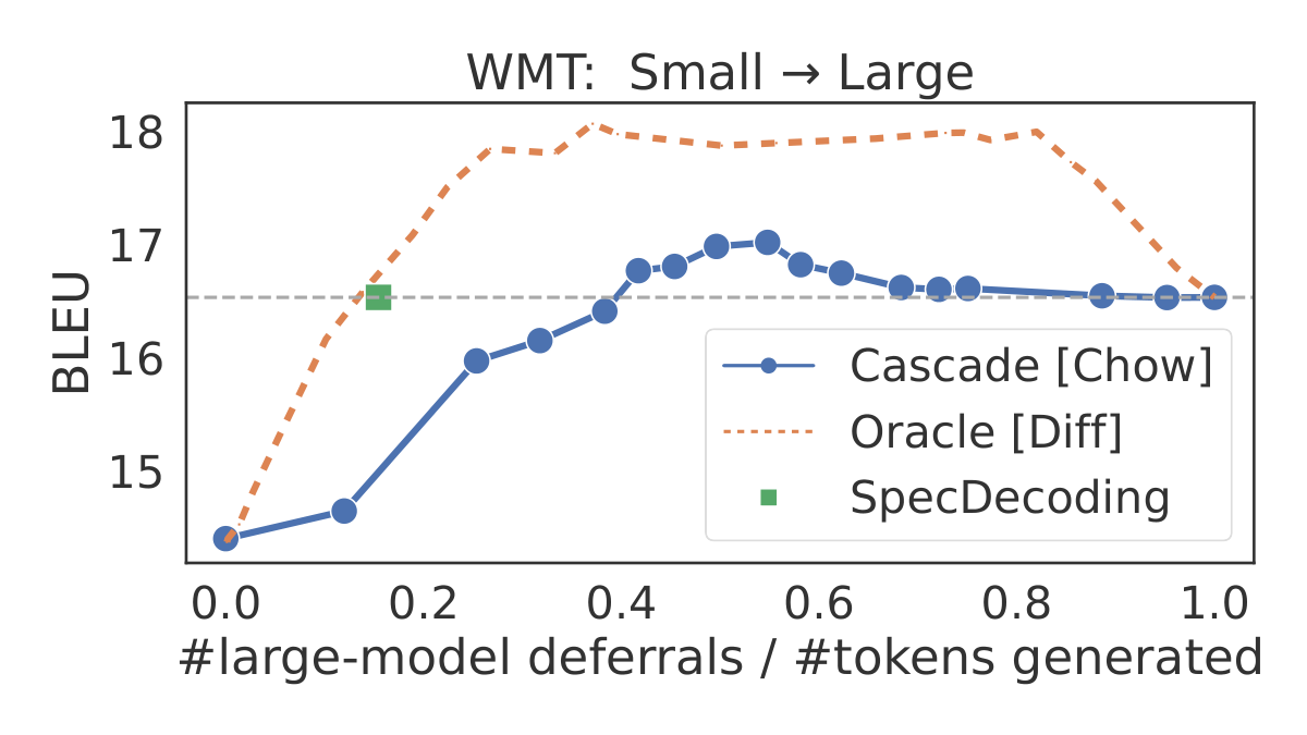
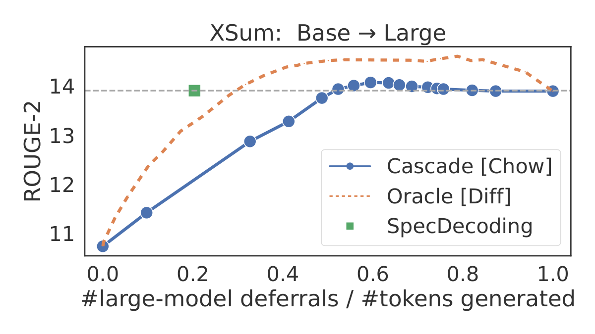
As a concrete example, we consider token-level cascades of T5 models ([35]) of two different sizes finetuned on a WMT EN →\rightarrow→ DE translation [39] and an extreme summarization (XSum) task ([40]). We construct these cascades using both (token-level) Chow's rule in Equation 2 and the oracle
Diff rule in Equation 5, and also apply speculative decoding with the smaller (larger) model as the drafter (verifier). In Figure 1, we plot quality as a function of fraction of samples deferred to the large model (number of deferrals divided by number of generated tokens), as we vary the cost parameter α\alphaα. Note that with speculative decoding, each verification step verifies γ\gammaγ tokens in parallel, but is counted as a single deferral to the large model. While speculative decoding matches the quality of the large model (right-most point), the oracle yields significantly better cost-qualty trade-offs. Even Chow's rule, which is sub-optimal for cascading ([30]), offers better trade-offs, and outperforms speculative decoding in a small region. As noted by [31], this may be attributed to the ensembling effect in a cascade.However, as also evident from the plots, token-level cascades require a significantly larger number of deferrals to the large model to achieve the same quality. This is because token-level cascades are executed sequentially: whenever qqq defers, we execute ppp once to generate one next token for the prefix accumulated so far, and the control transfers back to qqq. In contrast, speculative decoding runs ppp in scoring mode to verify γ\gammaγ draft tokens from qqq in parallel. Moreover, the stochastic verification algorithm in speculative decoding often results in fewer tokens from qqq getting rejected compared to the deterministic deferral rules used in a cascade. These observations motivate a natural question: given their complementary strengths, how can we leverage the best of both these techniques?
💭 Click to ask about this figure
4. Speculative Cascades: Leveraging the Best of Both Worlds
In addressing the above question, we present our main contribution: a principled approach to combining the better trade-offs cascades offer with the faster execution of speculative decoding.
4.1 Speculative decoding with general target distributions
We begin by considering a generic version of speculative sampling that seeks to mimic a general target distribution derived from the drafter's and verifier's distributions. In the proposed sampling procedure outlined in Algorithm 4, we sample tokens auto-regressively as before from the drafter's distribution. During the verification step, however, we do not compare the drafter's token probabilities against the verifier's distribution. Instead, we use a user-specified target distribution π=T(q,p)∈ΔV\pi = \mathbb{T}(q, p) \in \Delta_{\mathscr{V}}π=T(q,p)∈ΔV derived from the drafter's and verifier's distributions at position ttt, for some function T(⋅,⋅)\mathbb{T}(\cdot, \cdot)T(⋅,⋅) that is inexpensive to compute. We accept a draft token xtx_txt when q(xt)≤π(xt)q(x_t) \leq \pi(x_t)q(xt)≤π(xt) and reject it otherwise with probability 1−π(xt)q(xt)1 - \frac{\pi(x_t)}{q(x_t)}1−q(xt)π(xt). Upon rejection, we re-sample from the residual distribution norm(max{0,π(⋅)−q(⋅)})\operatorname{norm}\left(\max\{0, \pi(\cdot) - q(\cdot)\}\right)norm(max{0,π(⋅)−q(⋅)}).
This general procedure not only encompasses standard speculative decoding ([15]) for T(q,p)=p\mathbb{T}(q, p) = pT(q,p)=p, but also includes lossy speculative decoding ([32]) as a special case:
Lemma 3
Algorithm 4 reduces to the lossy speculative sampling procedure in ([32]) with parameters α\alphaα and β\betaβ when T(q,p)(v)=max{min{q(v),p(v)1−α},p(v)β}\mathbb{T}(q, p)(v) = \max\{\min\{ q(v), \frac{p(v)}{1 - \alpha} \}, \frac{p(v)}{\beta}\}T(q,p)(v)=max{min{q(v),1−αp(v)},βp(v)}.
4.2 From sequential to speculative cascades
Equipped with Algorithm 4, we now propose new cascading techniques that implement their deferral rule in a speculative manner. Recall from § 3.1 that a token-level cascade of two models qqq and ppp is defined by a deferral rule r:Vt−1→{0,1}r: \mathscr{V}^{t-1}\rightarrow \{0, 1\}r:Vt−1→{0,1}. For a prefix x<tx_{<t}x<t, the next-token distribution at position ttt modeled by this cascade can be written as:
In fact, for all the deferral rules described in § 2, the resulting distribution can be described by a target distribution function Tδ\mathbb{T}_\deltaTδ of the form:
for some function δ:ΔV×ΔV→{0,1}\delta: \Delta_\mathscr{V} \times \Delta_\mathscr{V} \rightarrow \{0, 1\}δ:ΔV×ΔV→{0,1} that maps distributions (q,p)(q, p)(q,p) to a binary decision. For example, for
Chow, δ(q,p)=1(maxvq(v)<1−α)\delta(q, p) = \bm{1}\big(\max_v q(v) < 1 - \alpha\big)δ(q,p)=1(maxvq(v)<1−α), and for Diff, δ(q,p)=1(maxvq(v)<maxvp(v)−α).\delta(q, p) = \bm{1}\big(\max_v q(v) < \max_v p(v) - \alpha\big).δ(q,p)=1(maxvq(v)<maxvp(v)−α). See Table 1 for a summary of target distributions for different deferral rules.Our proposal is to then invoke the speculative sampling procedure in Algorithm 4 with Tδ\mathbb{T}_\deltaTδ as the target distribution function. We outline this generic speculative cascading approach in Algorithm 5, and contrast it with the sequential execution of a deferral rule in Algorithm 2.
Remark 4: Exact implementation of oracle deferral rule {\tt Diff}
In a sequential cascade, the large model's distribution ppp cannot be used at the time the deferral decision is made (see Remark 2), as this would defeat the purpose of the cascade. With a speculative cascade, however, we can employ rules like
Diff that depend on both qqq and ppp. This is because we run the large model ppp in parallel on drafts generated by the small model qqq, allowing us to compute both p(⋅)p(\cdot)p(⋅) and q(⋅)q(\cdot)q(⋅) on every prefix.So far we have considered deferral rules designed for sequential cascades. In what follows, we derive the optimal deferral rule rrr for a speculative cascade, where we sample speculatively from a target distribution π=(1−r(x<t))⋅qt+r(x<t)⋅pt\pi = (1 - r(x_{<t})) \cdot q_t + r(x_{<t}) \cdot p_tπ=(1−r(x<t))⋅qt+r(x<t)⋅pt using qtq_tqt as the drafter.
4.3 Optimal speculative cascade deferral
As with sequential cascades (§ 2), we begin by defining an objective to minimize. We seek a deferral rule r:Vt−1→{0,1}r: \mathscr{V}^{t-1} \rightarrow \{0, 1\}r:Vt−1→{0,1} that minimizes a loss against the ground-truth distribution, while limiting the inference cost to be within a budget. (Per above, this deferral rule implicitly defines a target distribution π\piπ.) The inference cost crucially depends on how frequently a draft token is rejected in the verification phase, triggering a rollback. To this end, we derive the probability that a token sampled from qqq is rejected during verification, for a target distribution resulting from a deferral rule rrr.
Lemma 5
For a given prefix x<tx_{<t}x<t, and target distribution π=(1−r(x<t))⋅qt+r(x<t)⋅pt\pi = (1 - r(x_{<t})) \cdot q_t + r(x_{<t}) \cdot p_tπ=(1−r(x<t))⋅qt+r(x<t)⋅pt, the probability of a token drawn from draft distribution qtq_tqt being rejected is equal to:
r(x<t)⋅DTV(pt,qt),r(x_{<t}) \cdot D_{\textup{\textrm{TV}}}(p_t, q_t), r(x<t)⋅DTV(pt,qt),
where DTV(p,q)=∑v∈Vmax{0,p(v)−q(v)}D_\textup{\textrm{TV}}(p, q) = \sum_{v \in \mathscr{V}}\max\{0, p(v) - q(v)\}DTV(p,q)=∑v∈Vmax{0,p(v)−q(v)} is the TV distance between ppp and qqq.
Intuitively, whenever r(x<t)=0r(x_{<t}) = 0r(x<t)=0, π(v)=qt(v)\pi(v) = q_t(v)π(v)=qt(v), and therefore there is no rejection or roll-back; when r(x<t)=1r(x_{<t}) = 1r(x<t)=1, the rejection rate equals DTV(pt,qt)D_{\textup{\textrm{TV}}}(p_t, q_t)DTV(pt,qt).
For a fixed prefix x<tx_{<t}x<t, we formulate the goal of finding a solution to:
for some budget B>0B > 0B>0. Equivalently, one may minimize an unconstrained objective similar to Equation 3, for suitable cost parameter α>0\alpha > 0α>0 (see § C.4):
Contrasting Equation 8 with the deferral risk in Equation 3 for a sequential cascade, a key difference is that the cost of deferring to the larger model is no longer a constant, but depends on the similarity between qtq_tqt and ptp_tpt, as measured by the TV distance between them.
We next derive the optimal deferral rule for Equation 8, and construct a feasible estimator for it.
Lemma 6: {Optimal deferral for speculative cascades}
The minimizer of Equation 8 is of the form:
When ptp_tpt and qtq_tqt are similar, the rejection rate for qtq_tqt is low, and hence the deferral decision will depend largely on which of the two models yields a lower expected loss. When ptp_tpt and qtq_tqt are very different, the optimal decision is to defer to ptp_tpt only when it yields a substantially lower loss than qtq_tqt.
Plug-in estimator for Equation 9. The optimal rule requires estimating expectations with respect the ground-truth distribution P(⋅∣x<t).\mathbb{P}(\cdot|x_{<t}).P(⋅∣x<t). We employ similar plug-in estimators as the ones used with sequential cascades (§ 3). When ℓ=ℓ0-1\ell=\ell_\text{0-1}ℓ=ℓ0-1, we replace the expected 0-1 loss with (one minus) the maximum probability from the model, giving us:
The efficacy of the plug-in estimator depends on how closely the individual models approximate the ground-truth distribution P(⋅∣x<t)\mathbb{P}(\cdot|x_{<t})P(⋅∣x<t); this is formalized by the following regret bound:
Lemma 7: {Regret bound for }
Suppose ℓ=ℓ0-1\ell = \ell_{\emph{\text{0-1}}}ℓ=ℓ0-1. Then for a fixed prefix x<tx_{<t}x<t:
One can now run the speculative cascading procedure in Algorithm 5 using Equation 10 as the deferral rule; the corresponding δ(⋅)\delta(\cdot)δ(⋅) is listed in Table 1. See § C.2 for a similar derivation for ℓ=ℓlog\ell=\ell_{\log}ℓ=ℓlog.
4.4 Token-specific speculative cascades
The plug-in deferral rules in (Equation 5) and (Equation 10) decide between the drafter's distribution qt(⋅)q_t(\cdot)qt(⋅) and the verifier's distribution pt(⋅)p_t(\cdot)pt(⋅) by comparing their maximum token probabilities. A downside to this approach is that the draft token xt∼qt(⋅)x_t \sim q_t(\cdot)xt∼qt(⋅) may not maximize qt(⋅)q_t(\cdot)qt(⋅). Thus, even when xtx_{t}xt is of poor quality, we may end up accepting it because qtq_tqt happens to be more peaked than ptp_tpt.
To alleviate this problem, we propose the use of token-specific deferral rules r:Vt−1×V→{0,1}r: \mathscr{V}^{t-1} \times \mathscr{V} \rightarrow \{0, 1\}r:Vt−1×V→{0,1} that use both the prefix x<tx_{<t}x<t and a candidate token vvv to provide a binary decision r(x<t,v)∈{0,1}r(x_{<t}, v) \in \{0, 1\}r(x<t,v)∈{0,1}, with 0 indicating that the token is of acceptable quality. We may then construct a target distribution of the following form:
where η=∑v′∈Vr(x<t,v′)⋅qt(v′)\eta = \sum_{v' \in \mathscr{V}} r(x_{<t}, v') \cdot q_t(v')η=∑v′∈Vr(x<t,v′)⋅qt(v′) is a normalizing term chosen to ensure that ∑vπToken(v)=1\sum_v \pi_{\tt Token}(v) = 1∑vπToken(v)=1. This target distribution closely mimics qt(⋅)q_t(\cdot)qt(⋅) on tokens that the deferral rule rrr deems to be of acceptable quality, and defers to pt(⋅)p_t(\cdot)pt(⋅) otherwise. One can modify the generic speculative sampling algorithm in Algorithm 4 to use πToken\pi_{\tt Token}πToken as the target distribution, as shown in Algorithm 6 in § D.
To design rrr, we propose a heuristic variant of the
Diff rule in Equation 4 that compares the expected 0-1 loss from the candidate token vvv with the expected 0-1 loss from distribution ptp_tpt (in § D, we discuss deriving a similar variant of the OPT rule in Equation 9):for a cost parameter α\alphaα. The following are some simple plug-in approximations to Equation 12:
where we approximate P(v∣x<t)\mathbb{P}(v|x_{<t})P(v∣x<t) with either qt(v)q_t(v)qt(v) or pt(v)p_t(v)pt(v). Equation 15 is a multiplicative plug-in approximation that has similarities to the rejection criterion used by [15] for lossy speculative greedy decoding, and results in an intuitive target distribution:
where Topα={v∈V: pt(v) ≥ maxv′pt(v′)⋅(1−α)}\textup{Top}_\alpha = \{v \in \mathscr{V}:\, p_t(v) \, \geq\, \max_{v'} p_t(v') \cdot(1 - \alpha)\}Topα={v∈V:pt(v)≥maxv′pt(v′)⋅(1−α)} is the set of top ranked tokens by pt(⋅)p_t(\cdot)pt(⋅). For these top-ranked tokens, πTokenV3\pi_{\tt TokenV3}πTokenV3 approximates qt(⋅)q_t(\cdot)qt(⋅); for the rest, it is a re-scaled version of pt(⋅)p_t(\cdot)pt(⋅).
5. Further related work and conclusions
There has been a stream of work on improving the draft generation process in speculative decoding; these include having the drafter and verifier share the same backbone ([27, 41, 42, 43, 44, 45, 46, 47]), using multiple small draft models [48, 49], using tree-structured draft batches ([50, 51]), distilling the drafter with the verifier ([37]), and leveraging multiple sampled draft candidates [18].
The work that is most closely related to our specific proposal is the Big Little Decoder (BiLD)~([31]), which can be seen as another lossy variant of speculative decoding ([15, 32, 37]). BiLD has two phases: a fallback phase, during which the drafter qqq is run auto-regressively until its maximum predicted probability is sufficiently low; and a rollback phase, during which the verifier ppp is run in parallel on the prefixes generated by qqq and rolls back to the point where D(q,p)>αD(q, p) > \alphaD(q,p)>α, for a metric DDD that measures discrepancy and threshold α\alphaα. The fallback phase implements Chow's deferral rule in (Equation 2), and allows for the draft window size to vary dynamically based on an estimate of how likely the draft tokens will be accepted; the rollback phase can be seen as a deterministic variant of the rejection sampling algorithm of [15].
An advantage of BiLD over the rejection sampling algorithm in ([15]) is the use of Chow's rule to vary the draft window size. However, the final target distribution it seeks to mimic, TBiLD(q,p)(v)=1(D(q,p)≤α)⋅q(v)+1(D(q,p)>α)⋅p(v)\mathbb{T}_{\textup{BiLD}}(q, p)(v) = \bm{1}(D(q, p) \leq \alpha)\cdot q(v) + \bm{1}(D(q, p) > \alpha)\cdot p(v)TBiLD(q,p)(v)=1(D(q,p)≤α)⋅q(v)+1(D(q,p)>α)⋅p(v), is an approximation to ppp; specifically, the target distribution π=TBiLD(q,p)\pi = \mathbb{T}_{\textup{BiLD}}(q, p)π=TBiLD(q,p) is chosen to satisfy D(π,p)≤αD(\pi, p) \leq \alphaD(π,p)≤α. Hence, in cases where qqq deviates substantially from ppp, BiLD would choose ppp as the target distribution, even when qqq offers better quality on a prefix (where quality can be measured using a suitable loss function). In contrast, our proposed approach in § 4 uses speculative decoding to approximate target distributions that seek to optimally cascade between qqq and ppp. In our experiments, we compare the efficacy of using TBiLD\mathbb{T}_{\textup{BiLD}}TBiLD as the target distribution with the target distributions we propose in this paper (see Table 1).
💭 Click to ask about this figure
6. Experimental results
We compare our speculative cascading techniques with both sequential cascades and standard speculative decoding on a range of language benchmarks, including translation, reasoning, coding, QA, etc. We evaluate speculative cascades constructed from both the T5 v1.1 family of encoder-decoder models ([2]), and Gemma v2 decoder-only models ([34]). We construct the cascades with four deferral rules: (i)
Chow in (Equation 2), (ii) Diff in (Equation 5), (iii) OPT in (Equation 10), and (iv) the Token-specific rule in (Equation 15) (we present results for the V1 and V2 variants in § E.7).Cascades versus SpecDecode evaluation. Our evaluation protocol is markedly different from the standard evaluation of speculative decoding algorithms, where the goal is to speed up inference with a large model while preserving its output distribution. In contrast, our focus is on trading-off quality for lower inference costs by cascading two models of different sizes. We also do not claim to develop a new state-of-the-art method for fast LM inference. Furthermore, the speculative cascades we design build on the original speculative decoding algorithm [15]. While one could potentially also adapt our proposal to other recent variants of speculative decoding ([42, 52]), these involve a wholly orthogonal suite of techniques to what we propose (such as architectural changes, allowing for multiple drafts, distillation, and so on; see § 5).
Baselines. The cascading and speculative decoding methods we compare to include:
- Sequence-level cascade ([30, 25]) based on sequence-level Chow's rule in Equation 1 (
SeqCascade[Chow]). - Token-level cascade
outlined in Algorithm 2, with token-level Chow's rule in Equation 2 used for deferral ([33, 53]) (
TokenCascade[Chow]). - Lossy speculative decoding described in § 2, with both β=1\beta = 1β=1 ([15, 37]) (
SpecDecode[Lossy]) and β\betaβ tuned using the procedure in [32] (Lossy⋆^\star⋆). - Big-Little Decoder approach ([31]), with both the original deterministic version (
BiLD), and the variant where we apply Algorithm 4 to the target distribution TBiLD\mathbb{T}_{\textup{BiLD}}TBiLD in § 5 (BiLD∗^*∗).
Fine-tuned T5 cascades. Our experiments on T5 models are based on the setup in [37]; see § E.1 for details. We use T5-small (77M) as the small model, and either T5-large (800M) or T5-XL (3B) as the large model. In each case, we supervised fine-tune these models on three tasks: WMT EN →\rightarrow→ DE translation ([54]), CNN/DM summarization ([55]), and XSum abstractive summarization ([40]). We use temperatures T=0,0.1,0.5,1.0T=0, 0.1, 0.5, 1.0T=0,0.1,0.5,1.0, and block sizes γ=3,5,7\gamma = 3, 5, 7γ=3,5,7 (full results in § E). Following the protocol in [15, 37], to measure latency, we evaluate the wall-clock decoding time with batch size 1.
💭 Click to ask about this figure
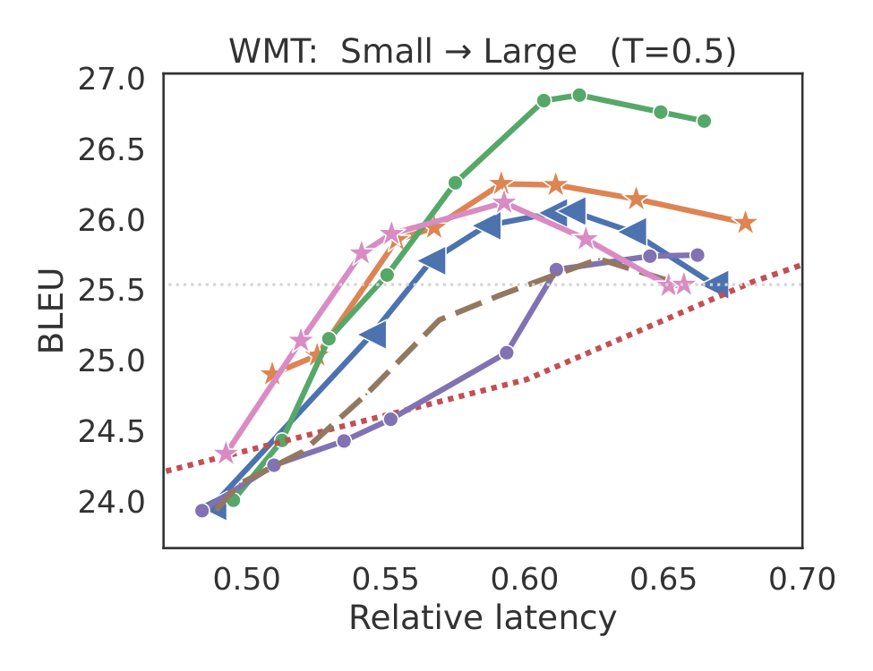
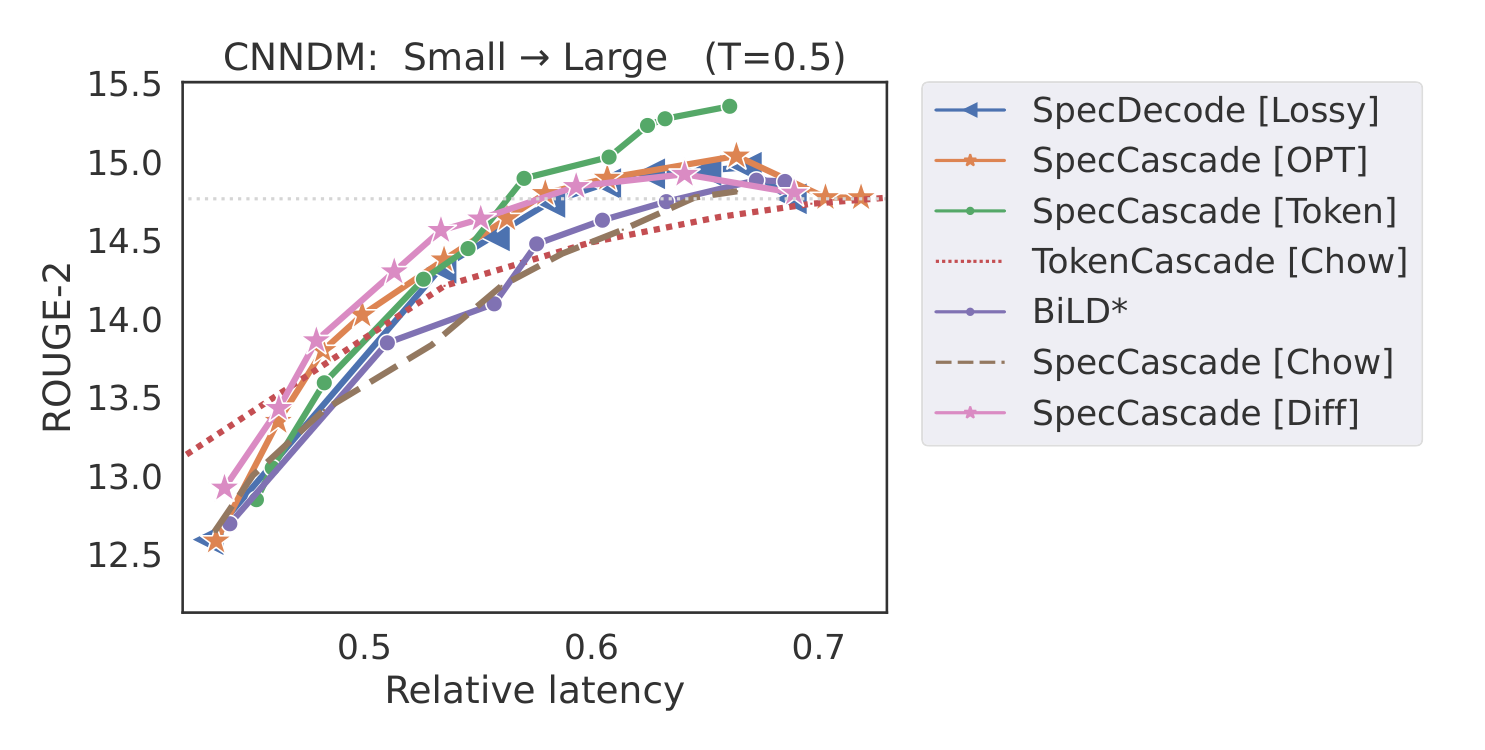
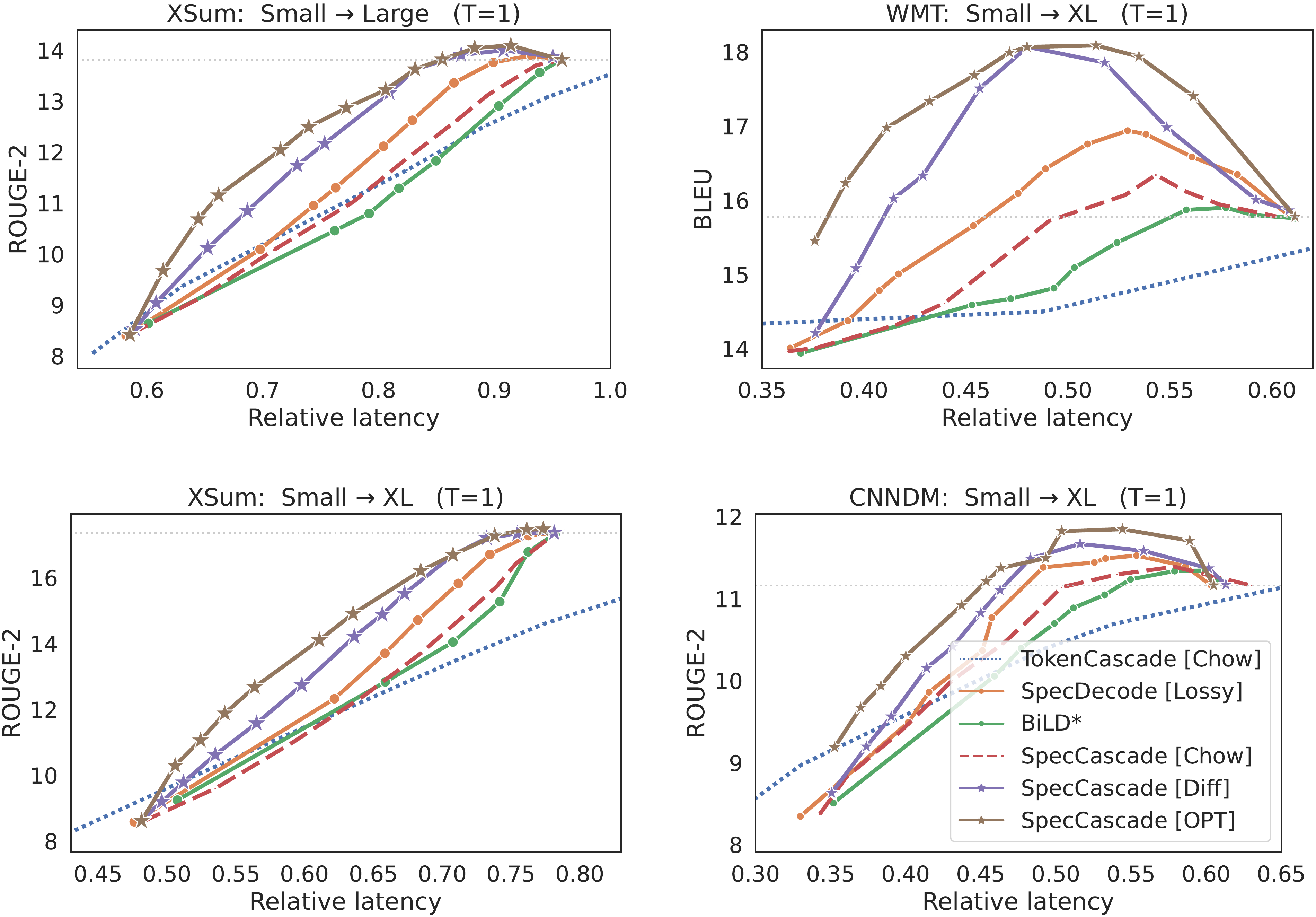
In Figure 2, we present plots of quality vs. latency for the different methods. In each case, we vary the lenience parameter α\alphaα, and plot either the BLEU or ROUGE-2 metric as a function of the relative latency to the larger model. For brevity, we include the three main baselines; in § E.5–Appendix E.6, we compare to
SpecDecode [Lossy⋆^\star⋆] ([32]) and the original BiLD algorithm [31]. Methods that use speculative execution are considerably faster than sequential token-level cascades (TokenCascade [Chow]), although sequential cascades do have an advantage in the low-latency regimes. This is because unlike speculative approaches, which always call the large model after every γ\gammaγ steps, a sequential cascade only invokes the large model when the small model defers.In Table 2, we report (i) the reduction in latency from T5 cascades when matching the quality of the large model, and (ii) the best quality that each method can deliver without exceeding the latency of the large model.
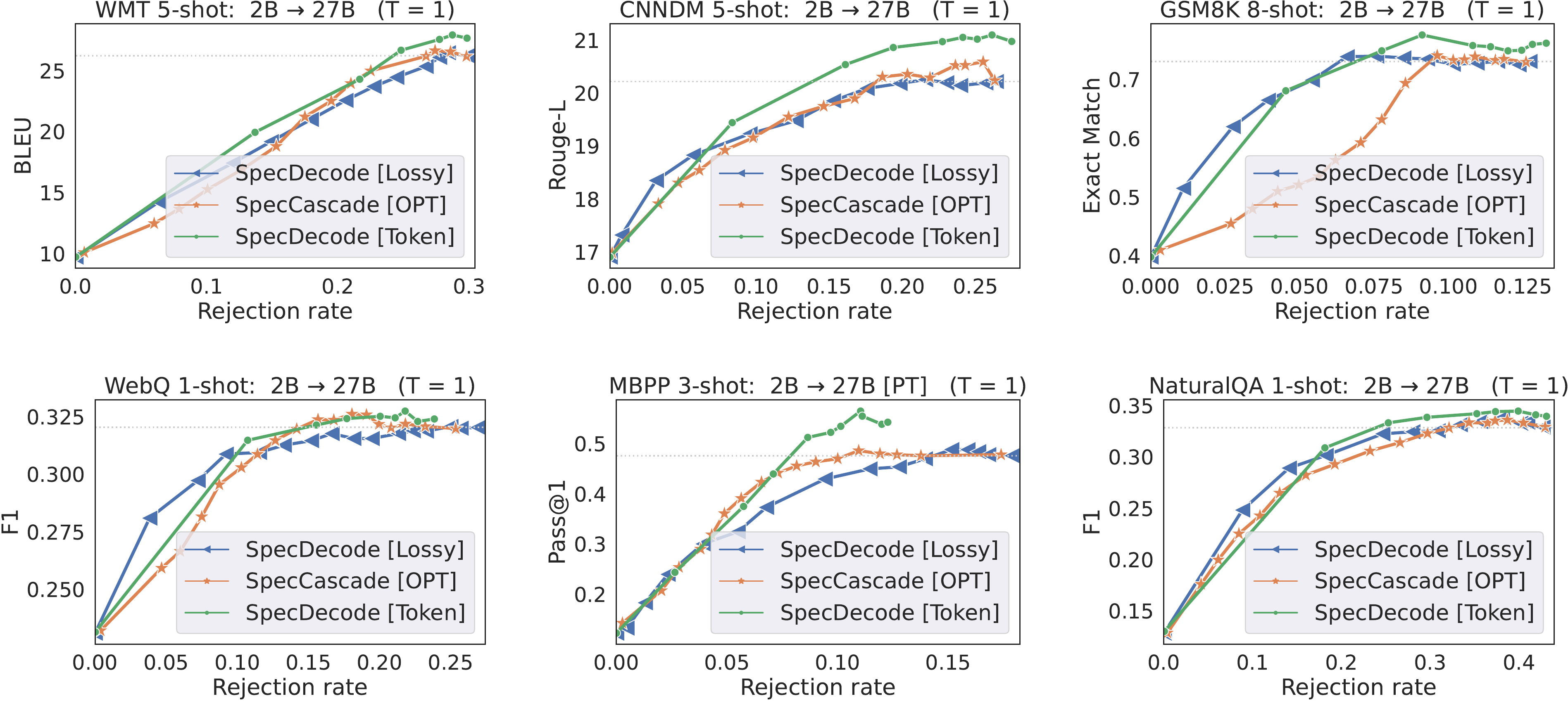
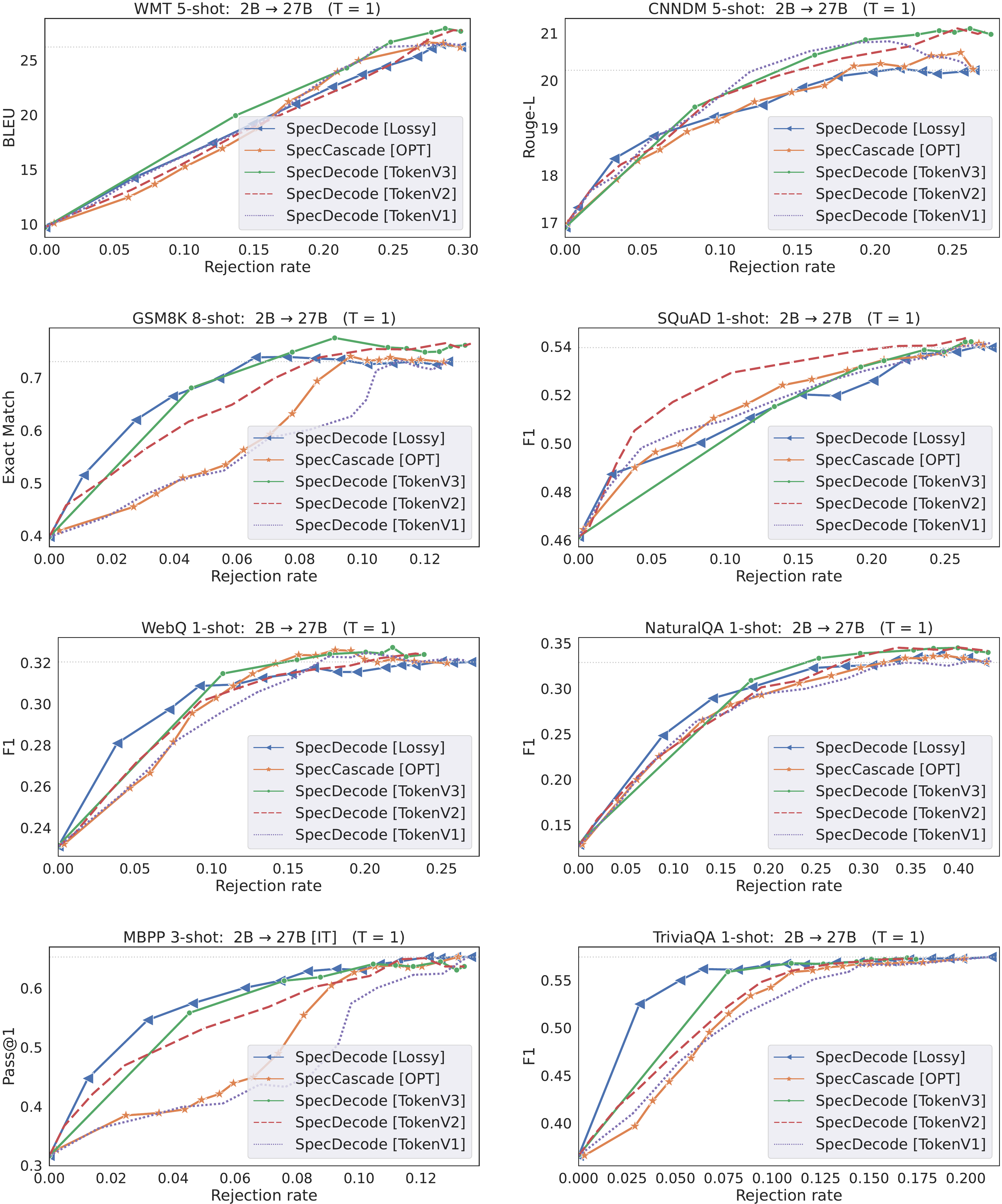
SpecCascade [Token] often yields the highest speed-up and the best quality metrics, with OPT coming in second. The cascading approaches are often seen to fare poorly on both quality and latency metrics, with the exception of WMT, where SeqCascade yields non-trivial speed-ups. The reason the Token-specific rule fares better than OPT and Diff is because the latter compute their deferral decisions based on which of qt(⋅)q_t(\cdot)qt(⋅) and pt(⋅)p_t(\cdot)pt(⋅) is more peaked; this can be a disadvantage when the sampled token is not close to the distribution mode, which is likely to happen with higher temperatures. As shown in § E.3, with lower temperatures, the gap between these rules diminishes.Few-shot Gemma cascades. To evaluate the Gemma model cascades, we use few-shot prompting with 8 language benchmarks: WMT, CNN/DM, GSM8K, MBPP, SQuAD 2.0, WebQuestions, NaturalQA and TriviaQA; many of these feature in the SpecBench suite ([56]). Figure 3 presents plots of quality vs. rejection rate with a 2B drafter and 27B verifier for γ=1\gamma=1γ=1. For brevity, we only compare the methods that fare the best in the previous experiments. With the exception of TriviaQA,
SpecCascade [Token] is able to both match the 27B's quality at a lower rejection rate and yield the best overall quality, often better than 27B. Since all three methods use the exact same implementation for speculative execution, a lower rejection rate directly translates to a lower latency.Interestingly,
OPT is not as effective as with T5. We attribute this to the differences in distributions between the two setups: with T5, the maximum token probability served as a good indicator of token accuracy for both qqq and ppp; with Gemma, we expect the large model to have a closer alignment with the ground-truth distribution (due to it being several billion parameters apart from the smaller model), and hence using the large model probabilities to measure confidence for both the small and large model (Equation 15) yields better trade-offs than comparing the modes from the two model distributions.7. Conclusions
We have proposed new speculative cascading techniques that use a combination of auto-regressive drafting and parallel verification to implement their deferral rule, and shown that they yield better cost-quality trade-offs than standard cascades and speculative decoding. A limitation of our approach is that while it offers a higher throughput, it also incurs a higher total compute cost compared to sequential cascades. In the future, we wish to replace our plug-in estimators with a router model ([25]) trained on ground-truth samples, to improve the local deferral objective at each position ttt (Equation 8) with a global objective, and to extend our proposal to more than two models.
Appendix
A. Proofs
A.1 Proof of Lemma 1
Proof: Expanding the loss in Equation 3, we have:
This objective is minimized by a deferral rule r:Vt−1→{0,1}r: \mathscr{V}^{t-1} \rightarrow \{0, 1\}r:Vt−1→{0,1} that minimizes, for each prefix x<tx_{<t}x<t, the term within the parenthesis. Therefore the minimizer r∗(x<t)=1r^*(x_{<t}) = 1r∗(x<t)=1 whenever the term within the parenthesis is negative:
and r∗(x<t)=0r^*(x_{<t}) = 0r∗(x<t)=0 otherwise. Re-arranging the terms completes the proof.
A.2 Proof of Lemma 3
Proof: The proof follows straight-forwardly from the results in ([32]). Recall from § 2 that the lossy speculative decoding procedure of ([32]) accepts a draft token xxx with probability:
and replaces a rejected draft token with a token sampled from the residual distribution:
for parameters α∈[0,1)\alpha \in [0, 1)α∈[0,1) and β≥1−α\beta \geq 1 - \alphaβ≥1−α.
We need to show that running Algorithm 4 with the target distribution:
results in the same acceptance probability Equation 16 and residual distribution Equation 17.
The acceptance probability for a draft token xxx when running Algorithm 4 on π\piπ is given by:
The corresponding residual distribution is given by:
We consider three possible cases:
Case (i): q(x)>11−α⋅p(x)≥1β⋅p(x)q(x) > \frac{1}{1 - \alpha}\cdot p(x) \geq \frac{1}{\beta}\cdot p(x)q(x)>1−α1⋅p(x)≥β1⋅p(x). In this case, π(x)=11−α⋅p(x)\pi(x) = \frac{1}{1 - \alpha}\cdot p(x)π(x)=1−α1⋅p(x). As a result:
Case (ii): 11−α⋅p(x)≥1β⋅p(x)>q(x)\frac{1}{1 - \alpha}\cdot p(x) \geq \frac{1}{\beta}\cdot p(x) > q(x)1−α1⋅p(x)≥β1⋅p(x)>q(x). In this case, π(x)=1β⋅p(x)\pi(x) = \frac{1}{\beta}\cdot p(x)π(x)=β1⋅p(x). As a result:
Case (iii): 11−α⋅p(x)≥q(x)≥1β⋅p(x)\frac{1}{1 - \alpha}\cdot p(x) \geq q(x) \geq \frac{1}{\beta}\cdot p(x)1−α1⋅p(x)≥q(x)≥β1⋅p(x). In this case, π(x)=q(x)\pi(x) = q(x)π(x)=q(x). As a result:
In all three cases, the acceptance probabilities and residual distributions are identical.
A.3 Proof of Lemma 5
Proof: Under a target distribution πt\pi_tπt, the probability of a draft token drawn from qtq_tqt being is rejected is given by ([15]):
Expanding π\piπ, the rejection probability becomes:
When r(x<t)=1r(x_{<t}) = 1r(x<t)=1, we have:
When r(x<t)=0r(x_{<t}) = 0r(x<t)=0, we have:
as desired.
A.4 Proof of Lemma 6
Proof: Expanding the deferral risk in Equation 8, we have:
This objective is minimized by a deferral rule r:Vt−1→{0,1}r: \mathscr{V}^{t-1} \rightarrow \{0, 1\}r:Vt−1→{0,1} that minimizes, for each prefix x<tx_{<t}x<t, the term within the parenthesis. Therefore the minimizer r∗(x<t)=1r^*(x_{<t}) = 1r∗(x<t)=1 whenever the term within the parenthesis is negative:
and r∗(x<t)=0r^*(x_{<t}) = 0r∗(x<t)=0 otherwise. Re-arranging the terms completes the proof.
A.5 Proof of Lemma 7
For a fixed prefix x<tx_{<t}x<t, we can write the deferral risk in Equation 8 as:
where CCC is a term independent of the deferral rule rrr. Let r∗:Vt−1→{0,1}r^*: \mathscr{V}^{t-1} \rightarrow\{0, 1\}r∗:Vt−1→{0,1} denote the optimal deferral rule that minimizes LspecL_{\rm spec}Lspec for any prefix x<tx_{<t}x<t. We then have:
Adding and subtracting maxvqt(v)−maxvpt(v)\max_{v} q_t(v) - \max_{v} p_t(v)maxvqt(v)−maxvpt(v) to the term within the second parenthesis, we get:
where we have used the fact that ∣r^OPT(x<t)−r∗(x<t)∣≤1.\left|\hat{r}_{\rm\tt OPT}(x_{<t}) - r^*(x_{<t})\right| \leq 1.∣r^OPT(x<t)−r∗(x<t)∣≤1.
We bound each term separately. For the first term, consider two cases: (i) maxvpt(v)+α⋅DTV(pt,qt)−maxvqt(v)≤0\max_{v} p_t(v) + \alpha \cdot D_{\textrm{TV}}(p_t, q_t) - \max_{v} q_t(v) \leq 0maxvpt(v)+α⋅DTV(pt,qt)−maxvqt(v)≤0 and (ii) maxvpt(v)+α⋅DTV(pt,qt)−maxvqt(v)>0\max_{v} p_t(v) + \alpha \cdot D_{\textrm{TV}}(p_t, q_t) - \max_{v} q_t(v) > 0maxvpt(v)+α⋅DTV(pt,qt)−maxvqt(v)>0. When (i) holds, r^OPT(x<t)=1\hat{r}_{\rm\tt OPT}(x_{<t}) = 1r^OPT(x<t)=1; so irrespective of whether r∗(x<t)r^*(x_{<t})r∗(x<t) is 0 or 1,
When (ii) holds, r^OPT(x<t)=0\hat{r}_{\rm\tt OPT}(x_{<t}) = 0r^OPT(x<t)=0; so irrespective of whether r∗(x<t)r^*(x_{<t})r∗(x<t) is 0 or 1,
Thus we have:
We next move to the second term. Since ℓ=ℓ0-1\ell=\ell_\text{0-1}ℓ=ℓ0-1, we have:
Suppose v∗∈arg maxvpt(v)v^* \in \operatorname{arg\, max}_v p_t(v)v∗∈argmaxvpt(v), then:
Similarly, we can show that:
Substituting Equation 19–Equation 21 in Equation 18 completes the proof.
B. Derivation of Chow's rule
We show below that Chow's rule is a plug-in estimator to the optimal solution to the following objective
where the deferral rule is penalized with a constant penalty α∈[0,1]\alpha \in [0, 1]α∈[0,1] for choosing to defer to the large model.
Following the same steps as Lemma 1, it is easy to show:
Lemma.
The minimizer of Equation 22 is of the form:
If ℓ=ℓ0-1\ell=\ell_\text{0-1}ℓ=ℓ0-1, one may employ a plug-in estimator to Equation 23 by replacing the expected 0-1 loss over qtq_tqt with 1−maxvqt(v)1 - \max_v q_t(v)1−maxvqt(v), giving us r^Chow(x<t)\hat{r}_{\rm \tt Chow}(x_{< t})r^Chow(x<t) in Equation 2. If ℓ=ℓlog\ell=\ell_{\log}ℓ=ℓlog, one may replace the expected log loss over qtq_tqt with the entropy of qtq_tqt, giving us:
where entropy(q)=−∑v∈Vq(v)⋅log(q(v)).\textrm{entropy}(q) = -\sum_{v \in \mathscr{V}} q(v) \cdot \log(q(v)).entropy(q)=−∑v∈Vq(v)⋅log(q(v)).
C. Optimal Deferral: Additional Discussion
We provide additional discussion for the optimal deferral rules derived in § 3 and § 4.
C.1 Optimal sequential deferral when ℓ=ℓlog\ell=\ell_{\log}ℓ=ℓlog
Recall that the optimal deferral rule for a sequential cascade in Lemma 1 takes the form:
When ℓ=ℓlog\ell = \ell_{\log}ℓ=ℓlog, we may use the entropy −∑vqt(v)⋅log(qt(v))-\sum_v q_t(v)\cdot \log(q_t(v))−∑vqt(v)⋅log(qt(v)) from qtq_tqt as an estimate of its expected log-loss, and similarly for ptp_tpt, giving us the plug-in estimator:
C.2 Optimal speculative deferral when ℓ=ℓlog\ell=\ell_{\log}ℓ=ℓlog
Recall that the optimal deferral rule for a speculative cascade in Lemma 6 takes the form:
When ℓ=ℓlog\ell=\ell_{\log}ℓ=ℓlog, one may construct a plug-in estimator for the above rule by replacing the expected log loss with the entropy from the distribution:
Lemma 8: {Regret bound for }
Suppose ℓ=ℓlog\ell = \ell_{\log}ℓ=ℓlog. Suppose for a fixed x<tx_{<t}x<t, ∣log(q(v))∣≤Bq|\log(q(v))| \leq B_q∣log(q(v))∣≤Bq and ∣log(p(v))∣≤Bp, ∀v∈V|\log(p(v))| \leq B_p, \, \forall v \in \mathscr{V}∣log(p(v))∣≤Bp,∀v∈V, for some Bq,Bp>0B_q, B_p > 0Bq,Bp>0. Then:
Proof: The proof follows similar steps to that for Lemma 7, except in bounding the resulting term2\text{term}_2term2 and term3\text{term}_3term3 for the log loss. In this case,
Similarly,
Plugging these bounds into the equivalent of Equation 18 in Lemma 7 for the log-loss completes the proof.
C.3 Optimal speculative deferral for greedy decoding
Lemma 9
When T→0T \rightarrow 0T→0, running Algorithm 5 with r~OPT\tilde{r}_{\rm\tt OPT}r~OPT as the deferral rule and q~t\tilde{q}_tq~t as the drafter is equivalent to running it with r^Diff\hat{r}_{\rm\tt Diff}r^Diff in Equation 5 as the deferral rule and q~t\tilde{q}_tq~t as the drafter.
Proof: Note that under greedy inference, q~t\tilde{q}_tq~t p~t\tilde{p}_tp~t are one-hot encodings of arg maxvqt(v)\operatorname{arg\, max}_v q_t(v)argmaxvqt(v) and arg maxvpt(v)\operatorname{arg\, max}_v p_t(v)argmaxvpt(v) respectively. As a result,
When running Algorithm 5 with r~OPT\tilde{r}_{\rm\tt OPT}r~OPT as the deferral rule, we will accept a draft token vvv with probability:
where δOPT(q,p) = 1(maxvq(v) < maxvp(v)−α⋅1(arg maxvq(v)≠arg maxvp(v)))\delta_{\rm OPT}(q, p) ~=~ \bm{1}\left(\max_{v} q(v) \, <\, \max_{v} p(v) - \alpha \cdot \bm{1}\left(\operatorname{arg\, max}_v q(v) \ne \operatorname{arg\, max}_v p(v)\right)\right)δOPT(q,p) = 1(maxvq(v)<maxvp(v)−α⋅1(argmaxvq(v)=argmaxvp(v))). When arg maxvq(v)=arg maxvp(v)\operatorname{arg\, max}_v q(v) = \operatorname{arg\, max}_v p(v)argmaxvq(v)=argmaxvp(v), then q~=p~\tilde{q} = \tilde{p}q~=p~, and irrespective of the outcome of δ(q,p),\delta(q, p), δ(q,p), we have that π(v)=1\pi(v) = 1π(v)=1. When arg maxvq(v)≠arg maxvp(v)\operatorname{arg\, max}_v q(v) \ne \operatorname{arg\, max}_v p(v)argmaxvq(v)=argmaxvp(v), then
When a token gets rejected, we sample a new token from the residual distribution:
When arg maxvq(v)=arg maxvp(v)\operatorname{arg\, max}_v q(v) = \operatorname{arg\, max}_v p(v)argmaxvq(v)=argmaxvp(v), pres(v)=0p_{\rm res}(v) = 0pres(v)=0. When arg maxvq(v)≠arg maxvp(v)\operatorname{arg\, max}_v q(v) \ne \operatorname{arg\, max}_v p(v)argmaxvq(v)=argmaxvp(v),
Thus both the acceptance probability and the residual distribution are the same as the one we would have used had we run Algorithm 5 with r^Diff\hat{r}_{\rm\tt Diff}r^Diff as the deferral rule.
C.4 Equivalence between Equation 7 and Equation 8
Since the prefix x<tx_{<t}x<t is fixed in Equation 7, the constrained optimization we seek to solve is of essentially of the following form:
for some coefficients c0,c1,c2>0c_0, c_1, c_2 > 0c0,c1,c2>0. Since rrr is a binary variable, we may formulate an equivalent unconstrained problem with the same minimizer:
where we choose α=0\alpha = 0α=0 when c2≤Bc_2 \leq Bc2≤B and choose an α>1c2⋅(c0−c1)\alpha > \frac{1}{c_2} \cdot (c_0 - c_1)α>c21⋅(c0−c1) otherwise. This unconstrained optimization problem is of the form in Equation 8.
D. Token-specific Speculative Cascade
We provide a modification of Algorithm 5 to accommodate the token-specific deferral rules in § 4.4.
Optimal token-specific deferral. Similar to § 4.3, we may consider deriving the optimal token-specific deferral rule. We start by formulating a similar optimization objective. For a fixed prefix x<tx_{<t}x<t, this would look like:
where πToken(v)=.(1−r(x<t,v))⋅qt(v)+η⋅pt(v)\pi_{\tt Token}(v) \stackrel{.}{=} (1 - r(x_{<t}, v)) \cdot q_t(v) + \eta \cdot p_t(v)πToken(v)=.(1−r(x<t,v))⋅qt(v)+η⋅pt(v) is the target distribution resulting from the choice of rrr, η=∑v′∈Vr(x<t,v′)⋅qt(v′)\eta = \sum_{v' \in \mathscr{V}} r(x_{<t}, v') \cdot q_t(v')η=∑v′∈Vr(x<t,v′)⋅qt(v′) is a normalization term, and B>0B > 0B>0 is a budget parameter.
However, unlike § 4.3, the above constrained optimization problem does not lend itself to a simple closed-form solution. In some highly simplistic special cases, we may be able to derive a solution. For example, suppose ℓ=ℓ0-1\ell=\ell_\text{0-1}ℓ=ℓ0-1, and the mode of qtq_tqt coincides with that of P(⋅∣x<t)\mathbb{P}(\cdot|x_{<t})P(⋅∣x<t), i.e., arg maxvqt(v)=arg maxvP(v∣x<t)\operatorname{arg\, max}_v q_t(v) = \operatorname{arg\, max}_v \mathbb{P}(v|x_{<t})argmaxvqt(v)=argmaxvP(v∣x<t); then the optimal token-specific rule is given by r(x<t,v)=0,r(x_{<t}, v) = 0, r(x<t,v)=0, for all v∈Vv \in \mathscr{V}v∈V.
Under more realistic cases, we may not be able to derive a solution as simple as the
OPT rule in Equation 10. Therefore, in our experiments, we employ the three heuristic rules in Equation 13–Equation 15, which are motivated by the form of the simpler Diff rule in Equation 5.E. Additional Experimental Details
We provide additional details about our experimental setup and additional experimental results. We will release code and an illustrative tutorial notebook along with the final manuscript.
💭 Click to ask about this figure
💭 Click to ask about this figure
E.1 Experimental setup and hyper-parameters
We elaborate on our experimental setup and the hyper-parameters used.
T5 datasets. For the WMT English to German translation task ([54]), we use a validation sample of size 3000 provided with the dataset. We set the maximum input length to 80 and the maximum output length to 80. For the Extreme Summarization (XSum) task ([40]), we use a validation sample of size 11305, and set the maximum input length to 1024 and the maximum output length to 64. For the CNN/Daily Mail summarization task ([55]), we use a validation sample of size 13368, and set the maximum input length to 2048 and the maximum output length to 128. Following ([37]), we use ROUGE-2 as the evaluation metric for the summarization tasks.
We note that [31] report ROUGE-L metrics for CNN/DM, which generally tend to evaluate to higher values than ROUGE-2. Furthermore, most of their experimental results are with greedy decoding (T=0T=0T=0), and hence, the ROUGE-L evaluation metrics they report in their paper tend to be higher for the same T5 models when compared to our numbers for ROUGE-2 with temperature sampling.
Gemma datasets. In addition to the WMT EN →\rightarrow→ DE translation and the CNN/DM summarization datasets, we use the GSM8K ([57]) math reasoning dataset, the MBPP ([58]) Python programming dataset, and four question-answering datasets: Natural Questions ([59]), TriviaQA ([60]), WebQuestions ([61]) and the Stanford Question-Answering Dataset (SQuAD) 2.0 ([62]). In each case, we sample 1000 prompts for evaluation. We employ few-shot inference, and set the maximum output length to 80 for WMT, to 128 for CNN/DM, to 320 for GSM8K and MBPP, and to 5 for all the question-answering datasets.
Models. We construct cascades from T5 v1.1 family of encoder-decoder models ([2]), of different sizes T5-small (77M), T5-base (250M), T5-large (800M) and T5-XL (3B).1 We follow the protocol in ([37]): we initialize with the public checkpoints, pre-train them further for 100K steps, and supervise finetune pre-trained models on the three respective tasks. We finetune them for a maximum of 250K steps on WMT, a maximum of 100K steps on XSum and a maximum of 200K steps on CNNDM.
The pre-trained checkpoints we use are available [here](https://console.cloud.google.com/ storage/browser/t5-data/pretrained_models).
We construct the Gemma cascades from instruction-tuned decoder-only v2 models. For MBPP alone we additionally experiment with pre-trained models. We use a 2B drafter, and either a 9B verifier or a 27B verifier ([34]).
Evaluation. For each dataset, we evaluate the quality metrics on the entire validation set. For the run-time analysis, we adopt the protocol followed in [15, 37]. We randomly sample 500 examples from the validation set, and calculate the wall-clock time taken for decoding with a batch size of 1. We repeat this for three trials and report the average running time. All methods are run on the same TPUv4 device. The drafter and verifier models are run without model parallelism.
Hyper-parameters. We set the block-size γ\gammaγ to 5 for all methods that use speculative execution. For the token-level cascades, we allow the small model to predict for a maximum of 10 tokens (similar to ([31])), before invoking the large model. This was needed, as otherwise, the small model would predict a long sequence, and when it eventually defers to the large model, the large model is bottle-necked by the pre-filling of the long prefix accumulated by the small model. We vary the lenience parameter α\alphaα to vary the latency and plot quality as a function of latency. We vary this parameter in the range 0 to 1 for all methods where the thresholding is on a probability metric; the exceptions to this are the BiLD variants, for which, we use a longer range, as detailed below.
BiLD baseline. For the BiLD method, we adopt the same discrepancy metric DDD as ([31]) for greedy decoding:
and pick the value of the threshold α\alphaα on this metric from the range [0,10][0, 10][0,10]. For temperature sampling with a non-zero temperature, we use the following natural analogue to the above DDD:
In § E.5, we present comparisons between different implementations of this method.
Lossy speculative decoding. See § E.6 for details.
E.2 Additional experimental plots
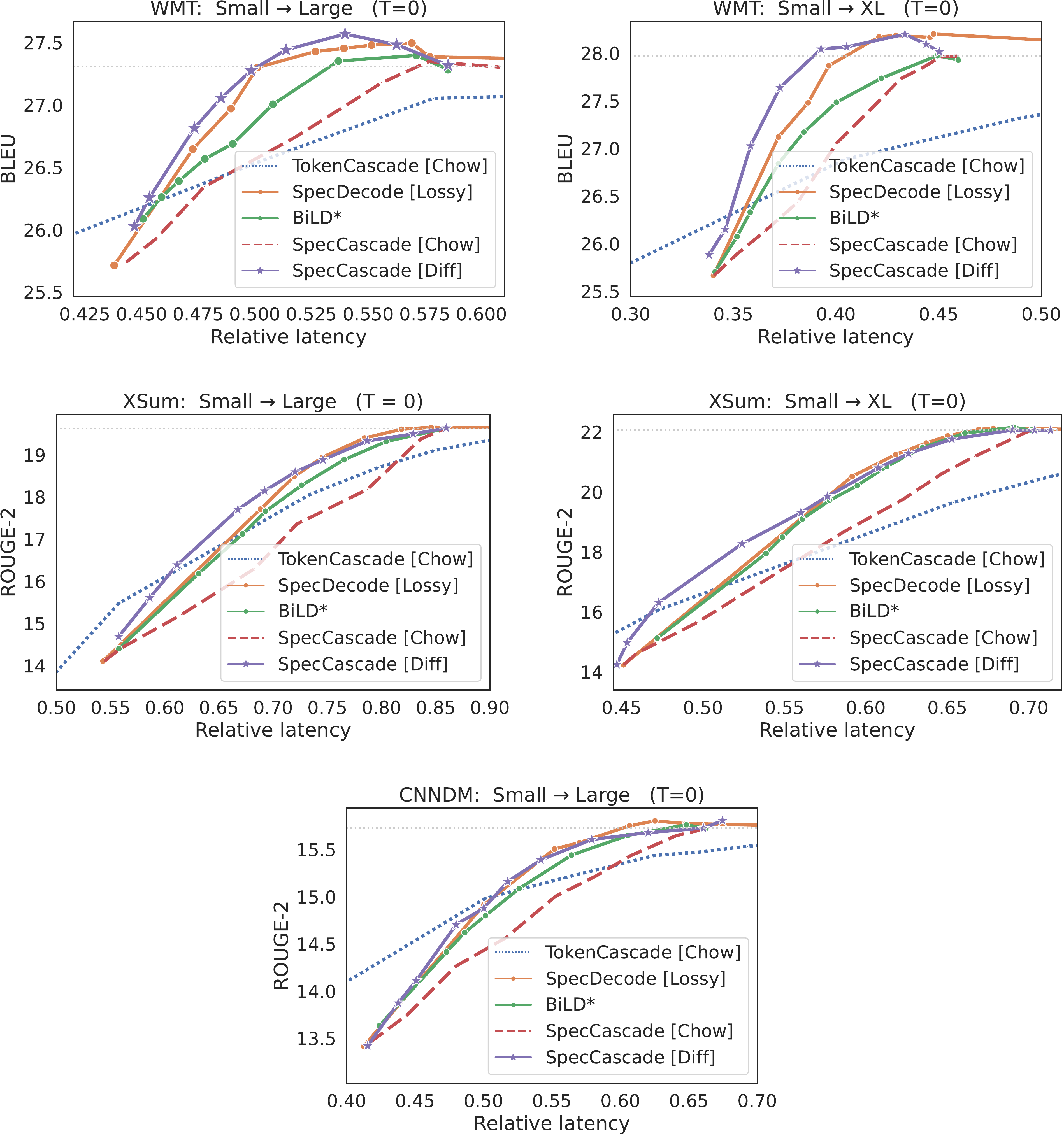
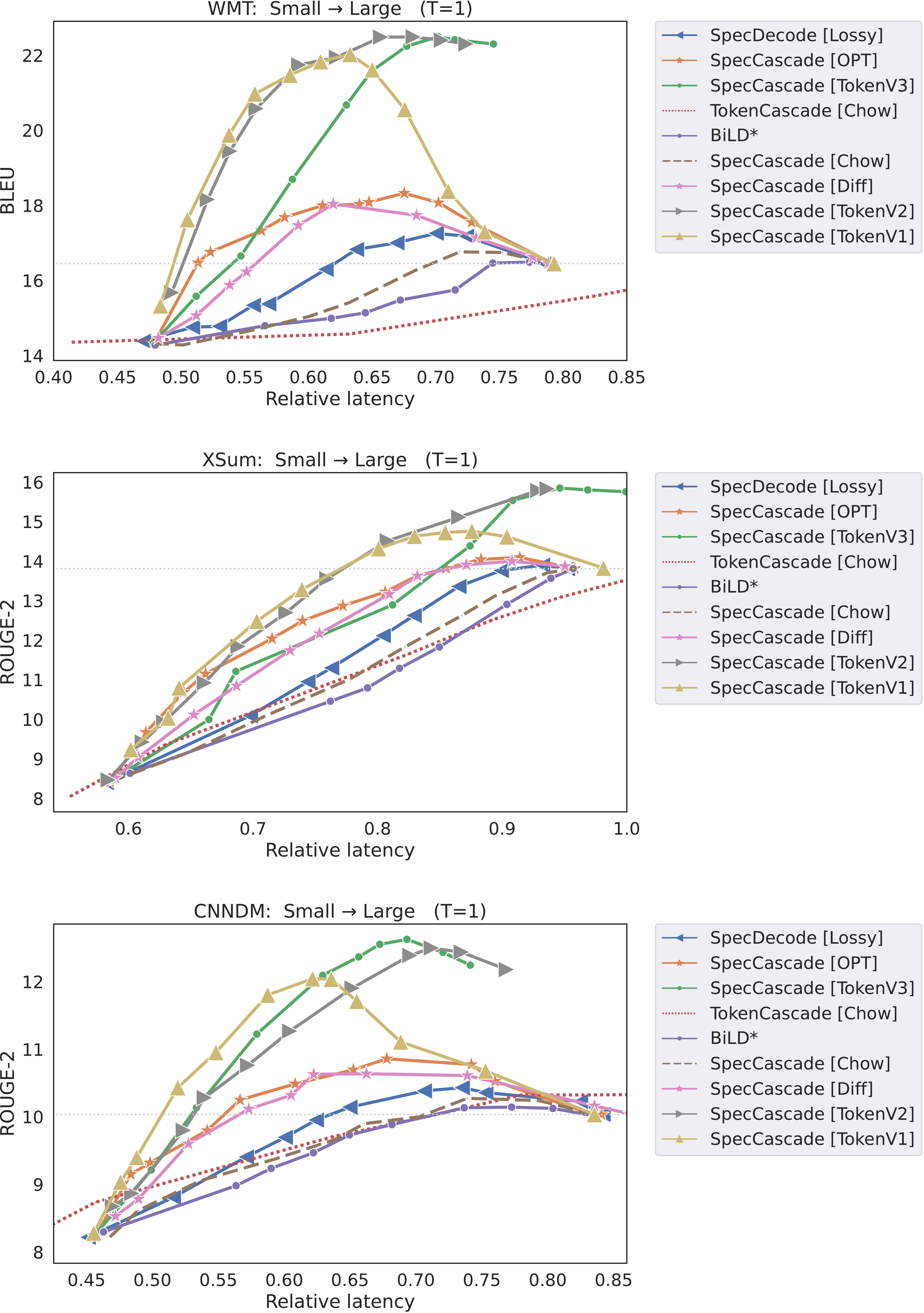
In Figure 4 and Figure 5, we provide additional plots of quality vs. latency for different inference strategies under temperature sampling (T=1T=1T=1) and greedy decoding respectively.
As noted in § C.3, with greedy decoding, the
OPT deferral rule coincides with the Diff deferral rule. When temperature T→0T \rightarrow 0T→0, DTV(p~t,q~t)=1D_{\textup{\textrm{TV}}}(\tilde{p}_t, \tilde{q}_t) = 1DTV(p~t,q~t)=1 whenever arg maxvpt(v)≠arg maxvqt(v)\operatorname{arg\, max}_v p_t(v) \ne \operatorname{arg\, max}_v q_t(v)argmaxvpt(v)=argmaxvqt(v), and is zero otherwise. In this case, running Algorithm 5 with r~OPT\tilde{r}_{\rm\tt OPT}r~OPT as the deferral rule (and q~t\tilde{q}_tq~t as the drafter) is equivalent to running it with r^Diff\hat{r}_{\rm\tt Diff}r^Diff in Equation 5 as the deferral rule. In other words, for greedy decoding, the optimal deferral rules for a speculative cascade coincides with that for a sequential cascade.Note that under greedy decoding, all methods yield better quality metrics compared to their performance under temperature sampling.
E.3 Comparing speculative deferral rules under different temperatures
In Figure 6, we present latency-quality trade-off plots for T5 cascades under temperature sampling with different temperatures. We compare lossy speculative decoding with two speculative cascade deferral rules:
OPT rule in Equation 5 and the Token-specific rule in Equation 15. We find that the gap between OPT and the Token-specific rule diminishes as the temperature decreases.The reason the
Token-specific rule fares better than OPT is because the latter compute their deferral decisions based on which of qt(⋅)q_t(\cdot)qt(⋅) and pt(⋅)p_t(\cdot)pt(⋅) is more peaked; this can be a disadvantage when the sampled token is not be close the distribution mode, which is likely to happen with higher temperatures. With lower temperatures, however, the sampled token is likely to be close the distribution mode, and as a result, the advantage that the Token-specific rule has over OPT diminishes.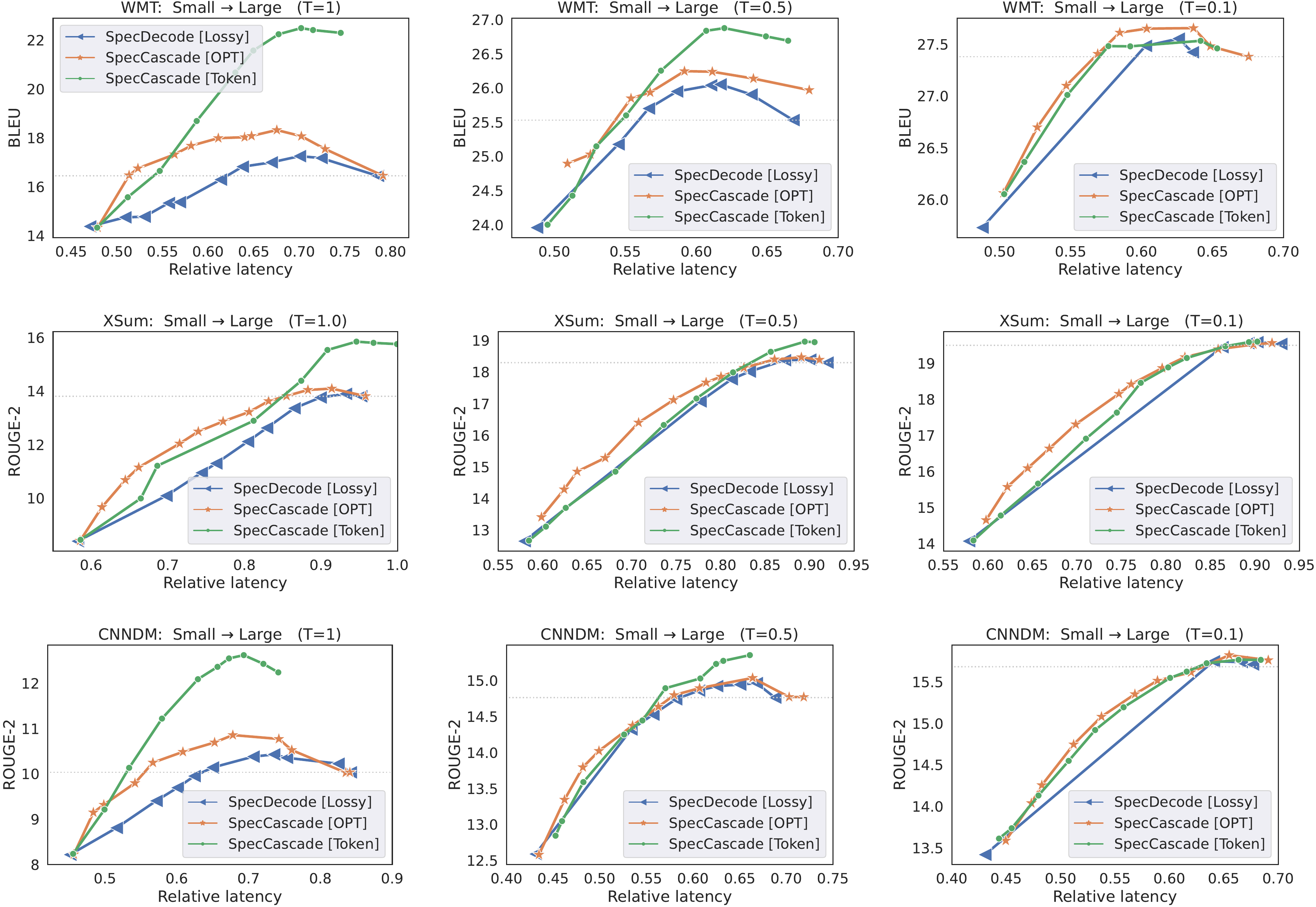
💭 Click to ask about this figure
E.4 Comparing speculative deferral rules under different block sizes γ\gammaγ
In Figure 7, we present latency-quality trade-off plots for T5 cascades under different block sizes γ\gammaγ. In each case, we find that the proposed speculative cascading techniques outperform lossy speculative decoding across different latency values. Furthermore, higher values of γ\gammaγ are seen to yield a wider range of trade-offs, with lower quality operating points shifting to the left, and better quality operating points shifting to the right. For example, with XSum,
SpecDecode [Lossy] with γ=3\gamma=3γ=3 matches the small model's quality at 0.64 relative latency, and matches the large model's quality at 0.85 relative latency; with γ=7\gamma=7γ=7, it matches the small model's quality at an even lower latency, but practically provides no speed-up when matching the larger model's quality. The reason a larger block size can hurt speed-up at the higher quality regime is because it can result in frequent rollbacks, thus defeating the purpose of using speculative execution.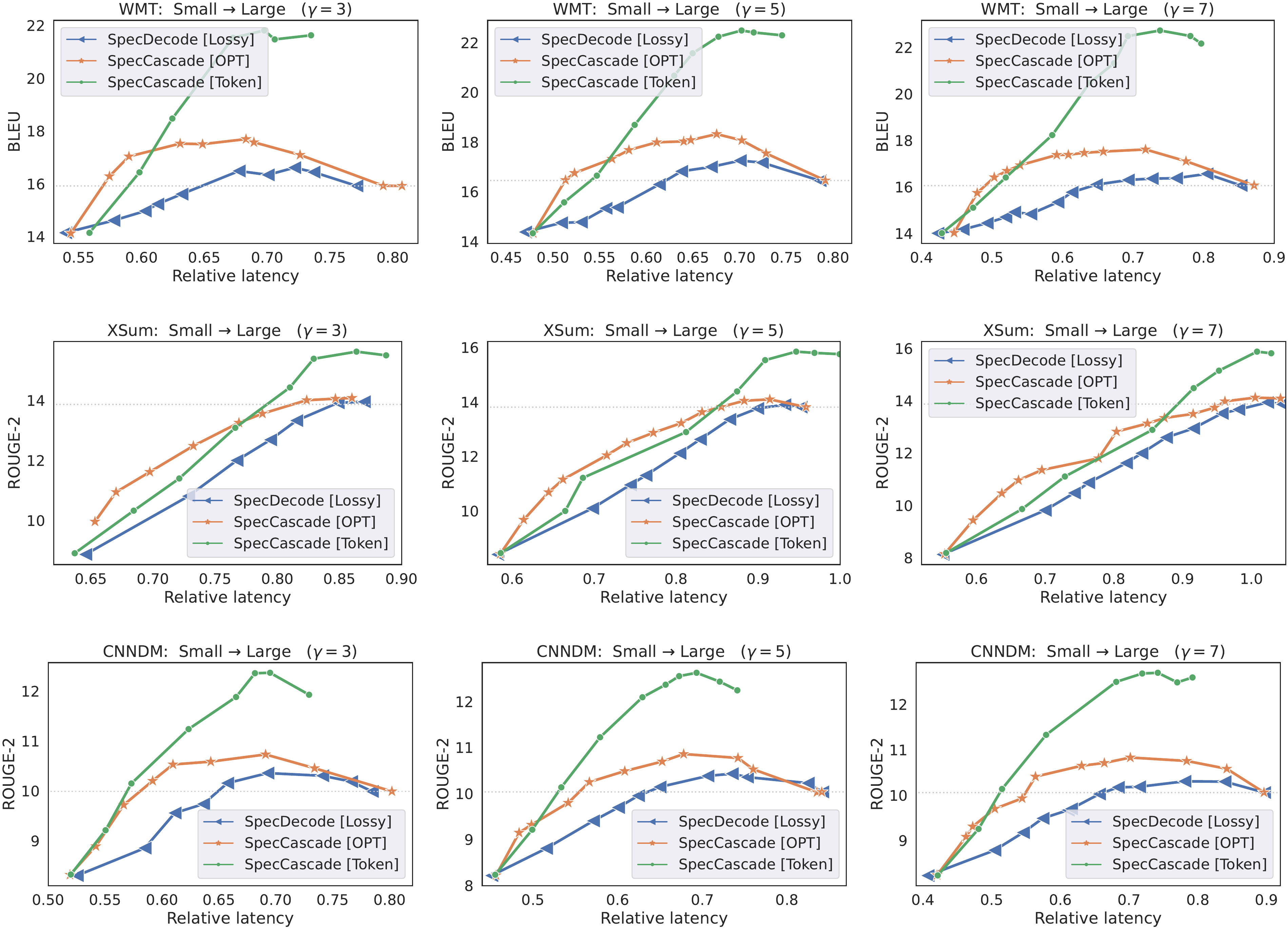
💭 Click to ask about this figure
![**Figure 8:** Top: Plots of quality vs. latency **comparing BiLD$^*$ with the original BiLD algorithm in [31]** with varying maximum draft window size $\gamma$ and fallback confidence threshold $\alpha_f$. Bottom: Comparison of lossy speculative decoding with $\beta=1$ [`Lossy`] and $\beta$ tuned using the procedure in ([32]) [`Lossy`$^\star$].](https://ittowtnkqtyixxjxrhou.supabase.co/storage/v1/object/public/public-images/xuwfvdjr/complex_fig_7149b40f0312.png)
💭 Click to ask about this figure
E.5 Big Little Decoder (BiLD) variants
In § 6, we compared against a version of the Big Little Decoder method ([31]) that applied Algorithm 4 to the target distribution TBiLD\mathbb{T}_{\textup{BiLD}}TBiLD the authors seek to mimic (§ 5). We now show that this version performs similarly to the original BiLD algorithm in ([31]).
A key difference to the original algorithm in ([31]) is the use of the fallback phase, where the drafter is run until its maximum predicted probability maxvq(v)<1−αf\max_v q(v) < 1 - \alpha_fmaxvq(v)<1−αf, for a threshold αf∈[0,1]\alpha_f \in [0, 1]αf∈[0,1] (or until a maximum block size of 10 is reached), and the use of a deterministic rollback policy where the verifier rejects a draft token whenever D(q,p)>αD(q, p) > \alphaD(q,p)>α. In our implementation, we adopt the speculative sampling algorithm from ([15]): we do not have the fallback policy and replace the determinisic rollback policy with the rejection sampling in Algorithm 4.
Figure 8 (top) compares the original version of BiLD with the version we use in § 6. We interleave between a T5-small and T5-large model on WMT, using greedy decoding (T=0T=0T=0) for inference. As prescribed by the authors ([31]), we use the following discrepancy metric for greedy decoding:
We compare our implementation (
BiLD∗^*∗), where we set the block size 5 (same as our proposed speculative cascading approaches) with the original BiLD for different choices of maximum block size γ\gammaγ and different fallback thresholds αf\alpha_fαf. For both methods, we vary the threshold α\alphaα on D(q,p)D(q, p)D(q,p) to vary the latency and plot the resulting BLEU score.A higher fallback threshold αf\alpha_fαf results in larger draft generation windows; this gives an advantage in the low latency regime, where most of the draft tokens are accepted. As a result,
BiLD [γ=10,α=0.9\gamma=10, \alpha=0.9γ=10,α=0.9] yields the lowest latencies, but also yields lower quality. A low fallback threshold results in very small draft generation windows, and consequently, in higher latencies. This is why BiLD [γ=5,α=0.1\gamma=5, \alpha=0.1γ=5,α=0.1] is the slowest but yields high quality metrics.Our implementation
BiLD∗^*∗ is seen to perform comparable to the best parameter choices for the original BiLD algorithm in Figure 8.Note: It is worth noting that while we view TBiLD\mathbb{T}_{\rm BiLD}TBiLD as the target distribution that algorithm in ([31]) seeks to mimic, the presence of the fallback phase could mean that on some inputs a output response is generated without the verification (or rollback) phase being invoked. In such cases, the output will be a sample from the drafter even if it turns out that it contains tokens for which D(qt,pt)>αD(q_t, p_t) > \alphaD(qt,pt)>α.
E.6 Lossy speculative decoding variants
In § 6, we compared against the lossy speculative decoding [32, 37] described in § 2, with the parameter β\betaβ set to 1. We now present results for this method with β\betaβ tuned according to the procedure in [32], and show that choosing β=1\beta=1β=1 fares at least as well as tuning β\betaβ.
The goal in [32] is to choose α\alphaα and β\betaβ so as to maximize the acceptance rate for the draft token, while ensuring that the KL divergence between the resulting target distribution and ppp is within an allowable limit RRR. The authors prescribe specifying RRR, and for each prefix, tuning α\alphaα and β\betaβ to solve the resulting constrained optimization problem. To be consistent with the rest of our experimental setup, we vary α\alphaα to vary the draft acceptance rate (note that each choice of α\alphaα corresponds to a particular KL divergence to ppp), and tune β≥1−α\beta \geq 1 - \alphaβ≥1−α to satisfy the following condition outlined in [32]:
We pick β\betaβ using a grid-search over 1000 values between α\alphaα and 10. Since this tuning procedure, in turn, can add to the method's latency, for a fair comparison, we analyze quality as a function of the fraction of calls to the large model. In Figure 8 (bottom), we plot these trade-off curves for loss speculative decoding with β=1\beta = 1β=1 (
Lossy) and for speculative decoding with β\betaβ tuned using the above procedure (Lossy$^{\star}$). We compare performances on WMT and XSum, and in each case, interleave a T5-small model with a T5-large model.In both cases, setting β=1\beta = 1β=1 provides trade-offs comparable to or better than using a tuned value of β\betaβ. The reason using a tuned value of β\betaβ fares worse than setting β=1\beta = 1β=1 might be because we are measuring quality in terms of BLEU or ROUGE-2, which is different from the KL divergence to ppp objective that the tuning procedure in [32] seeks to optimize.
E.7 Token-specific speculative cascades
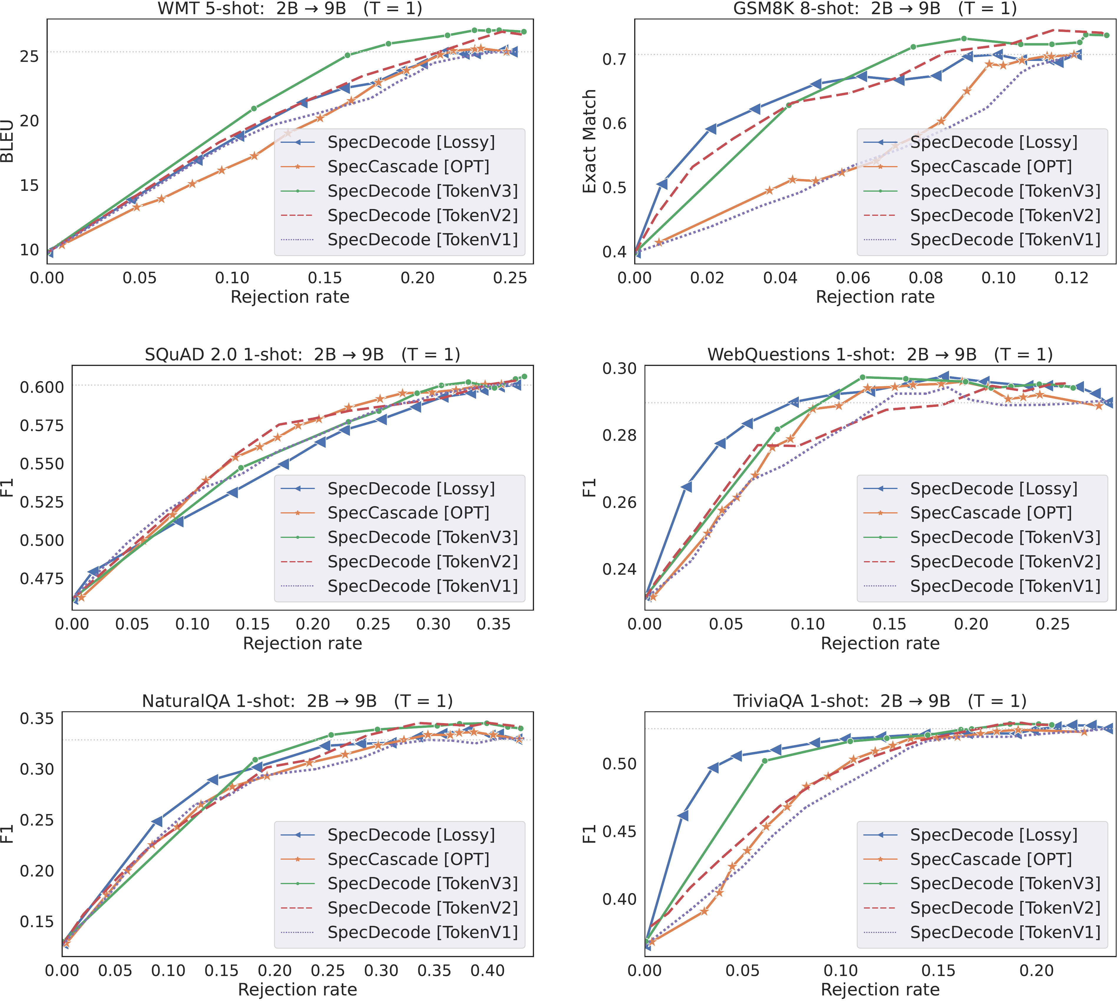
In Figure 9, we present latency-quality trade-off plots for cascades constructed from a T5 small and a T5 large model. We include in these comparisons, all three token-specific deferral rules in Equation 13–Equation 15. In Figure 10, we present trade-off plots for cascades constructed from Gemma 2B and Gemma 27B models with all three token-specific rules, and in Figure 11, we include similar plots for cascades constructed from Gemma 2B and Gemma 9B models. We note that the trends with the 2B →\rightarrow→ 9B are similar to those seen with the 2B →\rightarrow→ 27B cascades.
With the T5 models, the results are mixed, with the V1 and V2 variants sometime surpassing the V3 variant (which is the variant we included in the main experiments results in § 6) Interestingly, with the Gemma models, the V3 variant is seen to outperform the others for most rejection rates, with the exception of the 2B →\rightarrow→ 27B cascade on SQuAD 2.0, where the V2 variant is better.
The reason the V3 variant outperforms V1 and V2 on the Gemma models could be due to the fact that it uses the larger model's distribution pt(⋅)p_t(\cdot)pt(⋅) to measure confidence for both the drafter and verifier (see LHS and RHS in Equation 13). We expect this to be particularly helpful when there is a larger gap in sizes between qqq and ppp, and the larger model's distribution is better aligned with the ground-truth distribution compared to the smaller model. Furthermore, as noted in § 4.4, the multiplicative form of the rule results in a target distribution that has an intuitive form: it seeks to mimic qt(⋅)q_t(\cdot)qt(⋅) on the top- α\alphaα ranked tokens by pt(⋅)p_t(\cdot)pt(⋅) and uses a re-scaled version of pt(⋅)p_t(\cdot)pt(⋅) for the other tokens.
💭 Click to ask about this figure
💭 Click to ask about this figure
💭 Click to ask about this figure
F. Limitations
One of the limitations of our proposal is the use of plug-in estimators to approximate the optimal rule Equation 9. While these approximations are effective in practice, they rely on the individual models being calibrated. An alternative to the use of plug-in estimators is to use a router model explicitly trained to mimic the optimal rule using a validation sample drawn from P\mathbb{P}P ([25]). Another limitation is that the optimization objectives we seek to minimize are local objectives that seek to make the best deferral decision at the current position ttt. In doing so, they ignore the downstream effects of choosing a particular model in the current step. Devising a global deferral objective that takes downstream errors into account would be an interesting direction for future work. More broadly, our paper seeks to improve cost-quality trade-offs in LM inference. It is important that such improvements do not unfairly advantage one slice of the data or a subset of the population, at the cost of others. Ensuring that the trade-off gains that our approach offers is equitable across different slices of the data is another important direction for the future.
References
[1] Alec Radford, Karthik Narasimhan, Tim Salimans, Ilya Sutskever, et al. Improving language understanding by generative pre-training. https://cdn.openai.com/research-covers/language-unsupervised/language_understanding_paper.pdf 2018.
[2] Colin Raffel, Noam Shazeer, Adam Roberts, Katherine Lee, Sharan Narang, Michael Matena, Yanqi Zhou, Wei Li, and Peter J. Liu. Exploring the limits of transfer learning with a unified text-to-text transformer. J. Mach. Learn. Res., 21:140:1–140:67, 2020a. URL http://jmlr.org/papers/v21/20-074.html
[3] Tom Brown, Benjamin Mann, Nick Ryder, Melanie Subbiah, Jared D Kaplan, Prafulla Dhariwal, Arvind Neelakantan, Pranav Shyam, Girish Sastry, Amanda Askell, Sandhini Agarwal, Ariel Herbert-Voss, Gretchen Krueger, Tom Henighan, Rewon Child, Aditya Ramesh, Daniel Ziegler, Jeffrey Wu, Clemens Winter, Chris Hesse, Mark Chen, Eric Sigler, Mateusz Litwin, Scott Gray, Benjamin Chess, Jack Clark, Christopher Berner, Sam McCandlish, Alec Radford, Ilya Sutskever, and Dario Amodei. Language models are few-shot learners. In H. Larochelle, M. Ranzato, R. Hadsell, M. F. Balcan, and H. Lin (eds.), Advances in Neural Information Processing Systems, volume 33, pp.\ 1877–1901. Curran Associates, Inc., 2020.
[4] Sidney Black, Stella Biderman, Eric Hallahan, Quentin Anthony, Leo Gao, Laurence Golding, Horace He, Connor Leahy, Kyle McDonell, Jason Phang, Michael Pieler, Usvsn Sai Prashanth, Shivanshu Purohit, Laria Reynolds, Jonathan Tow, Ben Wang, and Samuel Weinbach. GPT-NeoX-20B: An open-source autoregressive language model. In Angela Fan, Suzana Ilic, Thomas Wolf, and Matthias Gallé (eds.), Proceedings of BigScience Episode #5 – Workshop on Challenges & Perspectives in Creating Large Language Models, pp.\ 95–136, virtual+Dublin, May 2022. Association for Computational Linguistics. doi:10.18653/v1/2022.bigscience-1.9. URL https://aclanthology.org/2022.bigscience-1.9
[5] Aakanksha Chowdhery, Sharan Narang, Jacob Devlin, Maarten Bosma, Gaurav Mishra, Adam Roberts, Paul Barham, Hyung Won Chung, Charles Sutton, Sebastian Gehrmann, Parker Schuh, Kensen Shi, Sasha Tsvyashchenko, Joshua Maynez, Abhishek Rao, Parker Barnes, Yi Tay, Noam Shazeer, Vinodkumar Prabhakaran, Emily Reif, Nan Du, Ben Hutchinson, Reiner Pope, James Bradbury, Jacob Austin, Michael Isard, Guy Gur-Ari, Pengcheng Yin, Toju Duke, Anselm Levskaya, Sanjay Ghemawat, Sunipa Dev, Henryk Michalewski, Xavier Garcia, Vedant Misra, Kevin Robinson, Liam Fedus, Denny Zhou, Daphne Ippolito, David Luan, Hyeontaek Lim, Barret Zoph, Alexander Spiridonov, Ryan Sepassi, David Dohan, Shivani Agrawal, Mark Omernick, Andrew M. Dai, Thanumalayan Sankaranarayana Pillai, Marie Pellat, Aitor Lewkowycz, Erica Moreira, Rewon Child, Oleksandr Polozov, Katherine Lee, Zongwei Zhou, Xuezhi Wang, Brennan Saeta, Mark Diaz, Orhan Firat, Michele Catasta, Jason Wei, Kathy Meier-Hellstern, Douglas Eck, Jeff Dean, Slav Petrov, and Noah Fiedel. PaLM: Scaling language modeling with pathways, 2022.
[6] Jason Wei, Maarten Bosma, Vincent Zhao, Kelvin Guu, Adams Wei Yu, Brian Lester, Nan Du, Andrew M. Dai, and Quoc V Le. Finetuned language models are zero-shot learners. In International Conference on Learning Representations, 2022. URL https://openreview.net/forum?id=gEZrGCozdqR
[7] Hyung Won Chung, Le Hou, Shayne Longpre, Barret Zoph, Yi Tay, William Fedus, Eric Li, Xuezhi Wang, Mostafa Dehghani, Siddhartha Brahma, Albert Webson, Shixiang Shane Gu, Zhuyun Dai, Mirac Suzgun, Xinyun Chen, Aakanksha Chowdhery, Sharan Narang, Gaurav Mishra, Adams Yu, Vincent Zhao, Yanping Huang, Andrew Dai, Hongkun Yu, Slav Petrov, Ed H. Chi, Jeff Dean, Jacob Devlin, Adam Roberts, Denny Zhou, Quoc V. Le, and Jason Wei. Scaling instruction-finetuned language models, 2022. URL https://arxiv.org/abs/2210.11416
[8] Yi Tay, Mostafa Dehghani, Vinh Q. Tran, Xavier Garcia, Jason Wei, Xuezhi Wang, Hyung Won Chung, Dara Bahri, Tal Schuster, Steven Zheng, Denny Zhou, Neil Houlsby, and Donald Metzler. UL2: Unifying language learning paradigms. In The Eleventh International Conference on Learning Representations, 2023. URL https://openreview.net/forum?id=6ruVLB727MC
[9] Rohan Anil and et al. PaLM 2 technical report, 2023.
[10] Hugo Touvron, Thibaut Lavril, Gautier Izacard, Xavier Martinet, Marie-Anne Lachaux, Timothée Lacroix, Baptiste Rozière, Naman Goyal, Eric Hambro, Faisal Azhar, Aurelien Rodriguez, Armand Joulin, Edouard Grave, and Guillaume Lample. Llama: Open and efficient foundation language models, 2023.
[11] Gemini Team, Rohan Anil, and et al. Gemini: A family of highly capable multimodal models, 2023.
[12] Maha Elbayad, Jiatao Gu, Edouard Grave, and Michael Auli. Depth-adaptive transformer. In International Conference on Learning Representations, 2020. URL https://openreview.net/forum?id=SJg7KhVKPH
[13] Reiner Pope, Sholto Douglas, Aakanksha Chowdhery, Jacob Devlin, James Bradbury, Anselm Levskaya, Jonathan Heek, Kefan Xiao, Shivani Agrawal, and Jeff Dean. Efficiently scaling transformer inference, 2022.
[14] Tal Schuster, Adam Fisch, Jai Gupta, Mostafa Dehghani, Dara Bahri, Vinh Q. Tran, Yi Tay, and Donald Metzler. Confident adaptive language modeling. In Alice H. Oh, Alekh Agarwal, Danielle Belgrave, and Kyunghyun Cho (eds.), Advances in Neural Information Processing Systems, 2022. URL https://openreview.net/forum?id=uLYc4L3C81A
[15] Yaniv Leviathan, Matan Kalman, and Yossi Matias. Fast inference from transformers via speculative decoding. In Andreas Krause, Emma Brunskill, Kyunghyun Cho, Barbara Engelhardt, Sivan Sabato, and Jonathan Scarlett (eds.), Proceedings of the 40th International Conference on Machine Learning, volume 202 of Proceedings of Machine Learning Research, pp.\ 19274–19286. PMLR, 23–29 Jul 2023. URL https://proceedings.mlr.press/v202/leviathan23a.html
[16] Charlie Chen, Sebastian Borgeaud, Geoffrey Irving, Jean-Baptiste Lespiau, Laurent Sifre, and John Jumper. Accelerating large language model decoding with speculative sampling. arXiv preprint arXiv:2302.01318, 2023a.
[17] Ying Sheng, Lianmin Zheng, Binhang Yuan, Zhuohan Li, Max Ryabinin, Beidi Chen, Percy Liang, Christopher Re, Ion Stoica, and Ce Zhang. FlexGen: High-throughput generative inference of large language models with a single GPU. In Andreas Krause, Emma Brunskill, Kyunghyun Cho, Barbara Engelhardt, Sivan Sabato, and Jonathan Scarlett (eds.), Proceedings of the 40th International Conference on Machine Learning, volume 202 of Proceedings of Machine Learning Research, pp.\ 31094–31116. PMLR, 23–29 Jul 2023. URL https://proceedings.mlr.press/v202/sheng23a.html
[18] Ziteng Sun, Ananda Theertha Suresh, Jae Hun Ro, Ahmad Beirami, Himanshu Jain, and Felix Yu. Spectr: Fast speculative decoding via optimal transport. Advances in Neural Information Processing Systems, 36, 2024.
[19] Xiaofang Wang, Dan Kondratyuk, Eric Christiansen, Kris M Kitani, Yair Alon, and Elad Eban. Wisdom of committees: An overlooked approach to faster and more accurate models. arXiv preprint arXiv:2012.01988, 2020.
[20] Jonathan Mamou, Oren Pereg, Moshe Wasserblat, and Roy Schwartz. TangoBERT: Reducing inference cost by using cascaded architecture, 2022. URL http://arxiv.org/abs/2204.06271
[21] Neeraj Varshney and Chitta Baral. Model cascading: Towards jointly improving efficiency and accuracy of nlp systems. arXiv preprint arXiv:2210.05528, 2022.
[22] Leila Khalili, Yao You, and John Bohannon. Babybear: Cheap inference triage for expensive language models, 2022. URL https://arxiv.org/abs/2205.11747
[23] David Dohan, Winnie Xu, Aitor Lewkowycz, Jacob Austin, David Bieber, Raphael Gontijo Lopes, Yuhuai Wu, Henryk Michalewski, Rif A. Saurous, Jascha Sohl-dickstein, Kevin Murphy, and Charles Sutton. Language model cascades, 2022. URL https://arxiv.org/abs/2207.10342
[24] Lingjiao Chen, Matei Zaharia, and James Zou. FrugalGPT: How to use large language models while reducing cost and improving performance, 2023b.
[25] Neha Gupta, Harikrishna Narasimhan, Wittawat Jitkrittum, Ankit Singh Rawat, Aditya Krishna Menon, and Sanjiv Kumar. Language model cascades: Token-level uncertainty and beyond. In The Twelfth International Conference on Learning Representations, 2024. URL https://openreview.net/forum?id=KgaBScZ4VI
[26] Dujian Ding, Ankur Mallick, Chi Wang, Robert Sim, Subhabrata Mukherjee, Victor Rühle, Laks V. S. Lakshmanan, and Ahmed Hassan Awadallah. Hybrid LLM: Cost-efficient and quality-aware query routing. In The Twelfth International Conference on Learning Representations, 2024. URL https://openreview.net/forum?id=02f3mUtqnM
[27] Mitchell Stern, Noam Shazeer, and Jakob Uszkoreit. Blockwise parallel decoding for deep autoregressive models. CoRR, abs/1811.03115, 2018. URL http://arxiv.org/abs/1811.03115
[28] Yuhui Li, Fangyun Wei, Chao Zhang, and Hongyang Zhang. EAGLE: Speculative sampling requires rethinking feature uncertainty. In International Conference on Machine Learning, 2024a.
[29] Heming Xia, Zhe Yang, Qingxiu Dong, Peiyi Wang, Yongqi Li, Tao Ge, Tianyu Liu, Wenjie Li, and Zhifang Sui. Unlocking efficiency in large language model inference: A comprehensive survey of speculative decoding, 2024a.
[30] Wittawat Jitkrittum, Neha Gupta, Aditya K Menon, Harikrishna Narasimhan, Ankit Rawat, and Sanjiv Kumar. When does confidence-based cascade deferral suffice? Advances in Neural Information Processing Systems, 36, 2023.
[31] Sehoon Kim, Karttikeya Mangalam, Suhong Moon, Jitendra Malik, Michael W Mahoney, Amir Gholami, and Kurt Keutzer. Speculative decoding with big little decoder. In Thirty-seventh Conference on Neural Information Processing Systems, 2023.
[32] Vivien Tran-Thien. An optimal lossy variant of speculative decoding, 2023. URL https://vivien000.github.io Unsupervised Thoughts (Blog). URL: https://github.com/vivien000/mentored_decoding
[33] C Chow. On optimum recognition error and reject tradeoff. IEEE Transactions on information theory, 16(1):41–46, 1970.
[34] Gemma Team, Morgane Riviere, Shreya Pathak, Pier Giuseppe Sessa, Cassidy Hardin, Surya Bhupatiraju, Léonard Hussenot, Thomas Mesnard, Bobak Shahriari, Alexandre Ramé, et al. Gemma 2: Improving open language models at a practical size. arXiv preprint arXiv:2408.00118, 2024.
[35] Colin Raffel, Noam Shazeer, Adam Roberts, Katherine Lee, Sharan Narang, Michael Matena, Yanqi Zhou, Wei Li, and Peter J Liu. Exploring the limits of transfer learning with a unified text-to-text transformer. Journal of machine learning research, 21(140):1–67, 2020b.
[36] Murong Yue, Jie Zhao, Min Zhang, Liang Du, and Ziyu Yao. Large language model cascades with mixture of thought representations for cost-efficient reasoning. In The Twelfth International Conference on Learning Representations, 2024. URL https://openreview.net/forum?id=6okaSfANzh
[37] Yongchao Zhou, Kaifeng Lyu, Ankit Singh Rawat, Aditya Krishna Menon, Afshin Rostamizadeh, Sanjiv Kumar, Jean-François Kagy, and Rishabh Agarwal. Distillspec: Improving speculative decoding via knowledge distillation. In The Twelfth International Conference on Learning Representations, 2024. URL https://openreview.net/forum?id=rsY6J3ZaTF
[38] Chuan Guo, Geoff Pleiss, Yu Sun, and Kilian Q. Weinberger. On calibration of modern neural networks. In Proceedings of the 34th International Conference on Machine Learning - Volume 70, ICML'17, pp.\ 1321–1330. JMLR.org, 2017.
[39] Ondřej Bojar, Christian Buck, Christian Federmann, Barry Haddow, Philipp Koehn, Johannes Leveling, Christof Monz, Pavel Pecina, Matt Post, Herve Saint-Amand, et al. Findings of the 2014 workshop on statistical machine translation. In Proceedings of the ninth workshop on statistical machine translation, pp.\ 12–58, 2014b.
[40] Shashi Narayan, Shay B Cohen, and Mirella Lapata. Don’t give me the details, just the summary! topic-aware convolutional neural networks for extreme summarization. In Proceedings of the 2018 Conference on Empirical Methods in Natural Language Processing, pp.\ 1797–1807, 2018.
[41] Taehyeon Kim, Ananda Theertha Suresh, Kishore Papineni, Michael Riley, Sanjiv Kumar, and Adrian Benton. Towards fast inference: Exploring and improving blockwise parallel drafts. arXiv preprint arXiv:2404.09221, 2024.
[42] Tianle Cai, Yuhong Li, Zhengyang Geng, Hongwu Peng, Jason D Lee, Deming Chen, and Tri Dao. Medusa: Simple LLM inference acceleration framework with multiple decoding heads. arXiv preprint arXiv:2401.10774, 2024.
[43] Giovanni Monea, Armand Joulin, and Edouard Grave. Pass: Parallel speculative sampling. arXiv preprint arXiv:2311.13581, 2023.
[44] Coleman Hooper, Sehoon Kim, Hiva Mohammadzadeh, Hasan Genc, Kurt Keutzer, Amir Gholami, and Sophia Shao. Speed: Speculative pipelined execution for efficient decoding. arXiv preprint arXiv:2310.12072, 2023.
[45] Jun Zhang, Jue Wang, Huan Li, Lidan Shou, Ke Chen, Gang Chen, and Sharad Mehrotra. Draft & verify: Lossless large language model acceleration via self-speculative decoding. arXiv preprint arXiv:2309.08168, 2023.
[46] Mostafa Elhoushi, Akshat Shrivastava, Diana Liskovich, Basil Hosmer, Bram Wasti, Liangzhen Lai, Anas Mahmoud, Bilge Acun, Saurabh Agarwal, Ahmed Roman, et al. Layer skip: Enabling early exit inference and self-speculative decoding. arXiv preprint arXiv:2404.16710, 2024.
[47] Fangcheng Liu, Yehui Tang, Zhenhua Liu, Yunsheng Ni, Kai Han, and Yunhe Wang. Kangaroo: Lossless self-speculative decoding via double early exiting. arXiv preprint arXiv:2404.18911, 2024.
[48] Ziyi Chen, Xiaocong Yang, Jiacheng Lin, Chenkai Sun, Jie Huang, and Kevin Chen-Chuan Chang. Cascade speculative drafting for even faster LLM inference. arXiv preprint arXiv:2312.11462, 2023c.
[49] Siqi Wang, Hailong Yang, Xuezhu Wang, Tongxuan Liu, Pengbo Wang, Xuning Liang, Kejie Ma, Tianyu Feng, Xin You, Yongjun Bao, et al. Minions: Accelerating large language model inference with adaptive and collective speculative decoding. arXiv preprint arXiv:2402.15678, 2024.
[50] Benjamin Spector and Chris Re. Accelerating LLM inference with staged speculative decoding. arXiv preprint arXiv:2308.04623, 2023.
[51] Xupeng Miao, Gabriele Oliaro, Zhihao Zhang, Xinhao Cheng, Zeyu Wang, Zhengxin Zhang, Rae Ying Yee Wong, Alan Zhu, Lijie Yang, Xiaoxiang Shi, et al. Specinfer: Accelerating large language model serving with tree-based speculative inference and verification. In Proceedings of the 29th ACM International Conference on Architectural Support for Programming Languages and Operating Systems, Volume 3, pp.\ 932–949, 2024.
[52] Yuhui Li, Fangyun Wei, Chao Zhang, and Hongyang Zhang. Eagle: Speculative sampling requires rethinking feature uncertainty. arXiv preprint arXiv:2401.15077, 2024b.
[53] Neha Gupta, Jamie Smith, Ben Adlam, and Zelda E Mariet. Ensembles of classifiers: a bias-variance perspective. Transactions of Machine Learning Research, 2022. URL https://openreview.net/forum?id=lIOQFVncY9
[54] Ondrej Bojar, Christian Buck, Christian Federmann, Barry Haddow, Philipp Koehn, Johannes Leveling, Christof Monz, Pavel Pecina, Matt Post, Herve Saint-Amand, Radu Soricut, Lucia Specia, and Ale s Tamchyna. Findings of the 2014 workshop on statistical machine translation. In Proceedings of the Ninth Workshop on Statistical Machine Translation, pp.\ 12–58, Baltimore, Maryland, USA, June 2014a. Association for Computational Linguistics. URL http://www.aclweb.org/anthology/W/W14/W14-3302
[55] Karl Moritz Hermann, Tomas Kocisky, Edward Grefenstette, Lasse Espeholt, Will Kay, Mustafa Suleyman, and Phil Blunsom. Teaching machines to read and comprehend. Advances in neural information processing systems, 28, 2015.
[56] Heming Xia, Zhe Yang, Qingxiu Dong, Peiyi Wang, Yongqi Li, Tao Ge, Tianyu Liu, Wenjie Li, and Zhifang Sui. Unlocking efficiency in large language model inference: A comprehensive survey of speculative decoding, 2024b.
[57] Karl Cobbe, Vineet Kosaraju, Mohammad Bavarian, Mark Chen, Heewoo Jun, Lukasz Kaiser, Matthias Plappert, Jerry Tworek, Jacob Hilton, Reiichiro Nakano, et al. Training verifiers to solve math word problems. arXiv preprint arXiv:2110.14168, 2021.
[58] Jacob Austin, Augustus Odena, Maxwell Nye, Maarten Bosma, Henryk Michalewski, David Dohan, Ellen Jiang, Carrie Cai, Michael Terry, Quoc Le, et al. Program synthesis with large language models. arXiv preprint arXiv:2108.07732, 2021.
[59] Tom Kwiatkowski, Jennimaria Palomaki, Olivia Redfield, Michael Collins, Ankur Parikh, Chris Alberti, Danielle Epstein, Illia Polosukhin, Jacob Devlin, Kenton Lee, Kristina Toutanova, Llion Jones, Matthew Kelcey, Ming-Wei Chang, Andrew M. Dai, Jakob Uszkoreit, Quoc Le, and Slav Petrov. Natural questions: A benchmark for question answering research. Transactions of the Association for Computational Linguistics, 7:452–466, 2019. doi:10.1162/tacl_a_00276. URL https://aclanthology.org/Q19-1026
[60] Mandar Joshi, Eunsol Choi, Daniel Weld, and Luke Zettlemoyer. TriviaQA: A large scale distantly supervised challenge dataset for reading comprehension. In Proceedings of the 55th Annual Meeting of the Association for Computational Linguistics (Volume 1: Long Papers), pp.\ 1601–1611, Vancouver, Canada, July 2017. Association for Computational Linguistics. doi:10.18653/v1/P17-1147. URL https://aclanthology.org/P17-1147
[61] Jonathan Berant, Andrew Chou, Roy Frostig, and Percy Liang. Semantic parsing on freebase from question-answer pairs. In Proceedings of the 2013 conference on empirical methods in natural language processing, pp.\ 1533–1544, 2013.
[62] Pranav Rajpurkar, Jian Zhang, Konstantin Lopyrev, and Percy Liang. SQuAD: 100,000+ questions for machine comprehension of text. In Proceedings of the 2016 Conference on Empirical Methods in Natural Language Processing, pp.\ 2383–2392, Austin, Texas, November 2016. Association for Computational Linguistics. doi:10.18653/v1/D16-1264. URL https://aclanthology.org/D16-1264