On Training in Imagination

Nadav Timor$^{*}$
Weizmann Institute of Science

Ravid Shwartz-Ziv
New York University

Micah Goldblum
Columbia University

Yann LeCun
New York University
AMI Labs

David Harel
Weizmann Institute of Science

Abstract

State-of-the-art model-based reinforcement learning methods train policies on imagined rollouts. These rollouts are trajectories generated by a learned dynamics model and are scored by a learned reward model, but without querying the true environment during policy updates. We study this training paradigm by quantifying how errors in learned dynamics and reward models affect returns and policy optimization. First, we extend the analysis of Asadi et al. [2018b] to MDPs with learned reward models, and derive the optimal sample allocation—the ratio of dynamics samples to reward samples that minimizes a bound on return error under power-law scaling assumptions. We identify lower Lipschitz constants of the learned dynamics, reward, and policy as a representation desideratum that tightens this bound, and we connect this perspective to the temporal-straightening objective of Wang et al. [2026]. Second, we examine how policy optimization with REINFORCE tolerates noisy rewards, which are often cheaper to obtain. We show that zero-mean reward noise leaves the gradient estimator unbiased and adds at most a variance term that decreases with the number of rollouts. This introduces a practical tradeoff: given a fixed budget, should one buy more rollouts with cheaper but noisier rewards, or fewer rollouts with more expensive but less noisy rewards? We reduce this choice to a one-dimensional optimization problem and characterize the optimum.

$^{*}$ Corresponding author: [email protected].

Preprint.

Executive Summary: This paper analyzes "training in imagination," a widely used approach in reinforcement learning where policies improve solely on simulated trajectories drawn from learned models of dynamics and rewards, without further interaction with the real environment. Leaders at organizations deploying autonomous systems face rising costs for data collection, human annotations, and simulation runs; these costs grow especially fast when reward signals come from experts or human preferences. The core open questions are how much performance suffers from each type of model error, how to split a fixed budget between the two data streams, and whether cheaper but noisier reward labels can be used without harming learning.

The authors set out to derive practical allocation rules and robustness guarantees under standard assumptions about error decay and model regularity, then to test those rules on controlled benchmarks. They extended existing error bounds to separate dynamics and reward contributions, proved that lower Lipschitz constants on the learned models tighten return-error guarantees, and reduced the budget-allocation problem to a simple ratio depending on per-sample costs and observed error-scaling rates. They also showed that the classical REINFORCE gradient estimator stays unbiased under additive zero-mean reward noise and quantified the resulting variance–cost tradeoff.

Three findings stand out. First, the performance gap decomposes cleanly into one term driven by reward-model error and another driven by dynamics-model error, each with its own controllable coefficient. Second, reward error typically falls nearly an order of magnitude faster with added data than dynamics error; consequently the optimal split often favors spending more on dynamics samples once reward cost exceeds a modest threshold. Third, averaging across trajectories removes variance from zero-mean reward noise but cannot correct systematic reward bias; choosing annotation fidelity therefore reduces to minimizing a one-dimensional cost-variance product whose shape dictates whether to buy quality, quantity, or one of the extremes.

These results matter because they turn an empirical tuning problem into a short, checkable calculation that directly informs data-acquisition contracts, annotation pipelines, and representation choices. Organizations can now decide in advance whether extra budget should go to cleaner labels, longer rollouts, or regularization that keeps model sensitivity low. In practice the savings come from avoiding both over-collection of expensive high-fidelity rewards and under-collection of the transitions that compound over long horizons.

Next steps are straightforward. Run a modest pilot that records realized value sensitivities on representative tasks rather than relying on global worst-case constants; use the measured sensitivities to set the initial sample ratio. At the same time, add lightweight regularization that penalizes rapid changes in latent velocity or output sensitivity and monitor whether the resulting models obey the tighter bounds predicted by the theory. Finally, re-evaluate the allocation rule whenever reward annotation costs or horizon length change materially.

The analysis assumes deterministic dynamics, power-law error scaling, and contraction conditions that hold in the tested regimes; the derived bounds are often loose by one to two orders of magnitude. Therefore treat the numerical ratios as directional guidance rather than precise prescriptions, and refresh them with fresh sensitivity measurements whenever the task distribution shifts.

1. Introduction

Section Summary: Recent advances show that agents can be trained effectively by generating imagined trajectories inside learned models of an environment’s dynamics and rewards, without any fresh interaction with the real system during the policy update. Existing theoretical guarantees, however, do not separately measure the harm caused by errors in the dynamics model versus errors in the reward model, nor do they indicate how a fixed sampling budget should be divided between the two. This paper supplies new bounds that attribute performance gaps to each source of error, identifies desirable properties of the learned representations, and gives explicit rules for allocating samples and tolerating noisy or biased reward labels.

In training in imagination, the policy is trained on rollouts generated by a learned dynamics model and scored by a learned reward model, with no environment interaction during the policy update step itself. Recent state-of-the-art instantiations include Dreamer 3 ([3]), trained across diverse control tasks with a single configuration, and Dreamer 4 ([4]), which extends the paradigm to long-horizon offline control. [5] earlier instantiate a closely related paradigm in board games and Atari, learning dynamics, reward, and value jointly.

These recent results provide strong empirical evidence that training in imagination can be effective on challenging control tasks. Existing simulation-lemma-style bounds ([6, 1]), however, do not assign independently controllable coefficients to dynamics-model and reward-model error, nor do they say how a sample budget should be split between dynamics samples and the typically more expensive reward samples (e.g., human preference labels in reinforcement learning from human feedback, or expert evaluation in robotics). The optimal trade-off between the two has not been theoretically characterized.

Four questions about this paradigm remain open. The first is error attribution: how much of the return gap comes from dynamics-model error versus reward-model error? The second is representation properties: what properties of the learned representations and the maps acting on them tighten the return-error bound? The third is budget allocation: given a fixed sample budget, how should it be split between dynamics transitions and reward annotations? The fourth is reward fidelity: how does $\textsc{reinforce}$ tolerate noisy or biased reward annotations, and when is it preferable to buy many cheap noisy annotations rather than fewer accurate ones?

Our contribution.

This paper treats the learned reward model as a separate source of error with its own sample budget, distinct from the learned dynamics, and quantifies the resulting attribution, allocation, and noise-tolerance trade-offs under Lipschitz and power-law assumptions.

1. Error attribution. Lemma 1 extends [1] by replacing the assumed ground-truth reward with a learned reward model, and gives a Lipschitz-based decomposition of the return gap with separable, independently controllable dynamics-error and reward-error coefficients.
2. Representation desiderata. Corollary 2 shows that the dynamics-error coefficient in Equation 1 is monotone non-decreasing in the Lipschitz constants $L_f, L_r, L_\pi$ of the learned dynamics, reward, and policy, identifying lower Lipschitz constants of the learned models as a representation desideratum. Proposition 4 couples this perspective to the temporal-straightening objective of [2], upper-bounding its curvature loss by a function of the Lipschitz constant of the latent velocity map.
3. Budget allocation. Theorem 5, under power-law error scaling for the dynamics and reward errors, gives a closed-form expression for the optimal ratio of dynamics samples to reward samples in terms of the power-law exponents, the per-sample costs, and the Lipschitz coefficient inherited from Lemma 1.
4. Reward fidelity. Theorem 6 shows that the multi-trajectory $\textsc{reinforce}$ estimator under additive zero-mean reward noise is unbiased with bounded variance inflation; Corollary 7 reduces the optimal-fidelity allocation problem to a one-dimensional minimization in the per-rollout annotation cost; and Proposition 8 formalizes systematic reward bias as a gradient bias that trajectory averaging cannot remove.

Empirical evaluations of the assumptions and predictions of these results appear in Section 3.1, Section 4.1, and Section 4.2.

Notation.

We write $\mathcal{M} = (\mathcal{S}, \mathcal{A}, f, r, \gamma)$ for a Markov decision process ($\textsc{mdp}$) with state space $\mathcal{S} \subseteq \mathbb{R}^{d_s}$, action space $\mathcal{A} \subseteq \mathbb{R}^{d_a}$, deterministic dynamics $f$, reward $r$, and discount $\gamma \in [0, 1)$. Starting from an initial state $s_0$, a policy $\pi$ generates a trajectory by $a_t = \pi(s_t)$ and $s_{t+1} = f(s_t, a_t)$. We write $J(\pi, \mathcal{M}) := \sum_{t=0}^{\infty} \gamma^t r(s_t, a_t)$ for the discounted return of $\pi$ in $\mathcal{M}$. Hats denote estimated quantities. In particular, $\hat{f}$ is the learned dynamics, $\hat{r}$ the learned reward, and $\hat{\mathcal{M}} = (\mathcal{S}, \mathcal{A}, \hat{f}, \hat{r}, \gamma)$ is the $\textsc{mdp}$ obtained by replacing $f$ and $r$ with $\hat{f}$ and $\hat{r}$. $\varepsilon_{\mathrm{dyn}} := \sup_{s, a} |\hat{f}(s, a) - f(s, a)|$ and $\varepsilon_{\mathrm{rew}} := \sup_{s, a} |\hat{r}(s, a) - r(s, a)|$ are the worst-case model errors. Throughout, $|\cdot|$ denotes the Euclidean norm.

2. Related work

Section Summary: Previous research on model-based reinforcement learning, such as the Dyna architecture and training-in-imagination methods, has used learned dynamics models to generate simulated experiences for policy training, usually treating those models and reward predictors as coupled components tuned through trial and error. Theoretical studies have derived bounds on the gap in returns between real and approximate environments based on transition and reward errors, while related work on data allocation has examined reward-free exploration phases or scaling laws that divide compute between model parameters and data. This section positions the current paper as extending those lines by separately tracking dynamics-model versus reward-model contributions to error, deriving an explicit budget split between the two data types, analyzing policy gradients under noisy or biased rewards, and connecting representation choices like latent straightening or Lipschitz regularization directly to long-horizon return accuracy.

Training a policy on rollouts from a learned model of the environment dates back to the Dyna architecture of [7], which interleaves real-environment transitions with updates on imagined transitions drawn from a learned dynamics model. Model-based policy optimization ([8]) uses short imagined rollouts from an ensemble dynamics model to augment policy updates. More recently, [3] train across diverse control tasks with a single learned world model and reward predictor, and [4] train agents inside scalable learned world models, calling this process "training in imagination". These works treat the learned dynamics model and the learned reward predictor as a single coupled object and tune it empirically; Appendix A reviews the broader latent-world-model lineage. Unlike the training-in-imagination lineage of [4], this paper decomposes return error into separate, independently controllable dynamics-model and reward-model terms (Lemma 1), derives a closed-form split of a single sample budget between dynamics transitions and reward annotations (Theorem 5), and characterizes the policy gradient inside this paradigm under both zero-mean noise and bias in the learned reward (Theorem 6 and Proposition 8).

Simulation return-error bounds have a long history in reinforcement learning theory, beginning with the simulation lemma of [6], which bounds the value gap between a true and approximate Markov decision process in terms of one-step transition and reward errors. Closest to our setting, [1] bound multi-step prediction error in model-based reinforcement learning under Lipschitz assumptions on the dynamics and policy, but they assume access to the ground-truth reward, so reward-model error never enters their bound. Appendix A surveys subsequent refinements of these bounds and value-aware model learning. Unlike [1], Lemma 1 carries a learned reward model through the analysis and produces an explicit reward-error term alongside the dynamics-error term with independently controllable coefficients, which is the structural ingredient that makes a budget split between dynamics and reward data well-posed.

Allocating sample budget between dynamics samples and reward samples sits at the intersection of reward-aware data collection and neural scaling laws. Reward-free exploration separates a reward-agnostic data-collection phase from later reward-conditioned planning, with sample-complexity guarantees that hold uniformly over downstream reward functions ([9]). Neural scaling laws fit power-law decays of loss in data and parameters ([10]) and, in the compute-optimal regime, split a single training budget between model parameters and tokens ([11]). Appendix A discusses related work on active observation, simulation budget allocation, and scaling laws specific to reinforcement learning and world-model pre-training. Unlike [11], Theorem 5 splits a single sample budget between two heterogeneous data streams—dynamics transitions and reward annotations—whose errors obey separately fitted power-law exponents, and yields a closed-form ratio in those exponents, the unit costs, and the Lipschitz coefficient inherited from Lemma 1.

Policy-gradient analysis under noisy rewards begins with the $\textsc{reinforce}$ estimator of [12]. A line of work studies robustness to reward corruption: [13] analyze adversarial corruption in which an $\varepsilon$-fraction of episodes have their rewards or transitions arbitrarily modified and develop estimators with provable robustness guarantees. [14] treat asymmetric verifier noise with false positives and false negatives in reinforcement learning with verifiable rewards. A parallel literature documents Goodhart-style overoptimization of learned reward models, in which the gap between proxy and gold rewards grows with optimization budget ([15]), a systematic failure mode rather than zero-mean reward noise. Appendix A reviews the policy-gradient and variance-reduction lineage and the broader reward-modeling literature. Unlike the adversarial setting of [13], Theorem 6 and Corollary 7 treat zero-mean i.i.d. reward noise as a per-rollout fidelity cost, which reduces annotation-budget allocation to a one-dimensional problem. Proposition 8 addresses reward bias separately, showing that any non-zero reward-bias gradient survives trajectory averaging.

The choice of latent representation, and the regularity of the maps acting on it, governs how reliably an imagined rollout tracks reality. [16] advocates joint-embedding predictive architectures, in which prediction takes place in a learned latent space rather than at the level of raw observations. [2] propose a temporal-straightening loss that encourages consecutive latent differences along a rollout to be parallel, so that long-horizon predictions in latent space follow a near-linear trajectory. On the regularization side, [17] introduce spectral normalization, which controls the Lipschitz constant of a neural network by normalizing the spectral norm of each weight matrix; Appendix A discusses related joint-embedding instantiations and Lipschitz-regularization mechanisms. These representation-learning and Lipschitz-regularization proposals are motivated by stability or representational quality, and their connection to long-horizon policy value is left implicit. Unlike [2] and [17], Corollary 2 and Proposition 4 couple these representation-learning desiderata to an explicit return-error coefficient, showing that the dynamics-error coefficient is monotone in the Lipschitz constants of the learned dynamics, reward, and policy and that the temporal-straightening loss is upper-bounded by a function of the latent-velocity-map Lipschitz constant.

3. Properties of representations for training in imagination

Section Summary: The section explains that effective representations for model-based planning should use latent states rather than raw observations, because doing so can reduce the Lipschitz constants of the learned dynamics, reward, and policy models. Lower Lipschitz constants shrink the theoretical bound on return error between the true and imagined environments, assuming model inaccuracies stay fixed. The same perspective accounts for the benefits of temporal-straightening objectives, which keep latent-state changes smooth and thereby further limit sensitivity.

What makes a representation of the system useful for training in imagination? [16] hypothesized that designing the dynamics, reward, and policy models to operate on latent states $z_t$ that capture a higher-level representation of the system—in place of raw observations $s_t$ and past actions $a_t$ —may improve prediction and planning across different time horizons. However, what properties such a representation should have has remained an open question. Lemma 1 and Corollary 2 give one answer to this open question: representations that lower the Lipschitz constants of the learned models tighten our bound on return error.

Similar to [1], we assume that the dynamics $f$, reward $r$, and policy $\pi$ satisfy the following Lipschitz conditions:

• $f$ is $L_f$-Lipschitz: $|f(s, a) - f(s', a')| \leq L_f(|s - s'| + |a - a'|)$ for all $s, s', a, a'$.
• $r$ is $L_r$-Lipschitz: $|r(s, a) - r(s', a')| \leq L_r(|s - s'| + |a - a'|)$ for all $s, s', a, a'$.
• $\pi$ is $L_\pi$-Lipschitz: $|\pi(s) - \pi(s')| \leq L_\pi|s - s'|$ for all $s, s'$.

########## {caption="Lemma 1: Simulation error decomposition"}

Let $\mathcal{M}, \hat{\mathcal{M}}$ be $\textsc{mdp}$ s sharing $(\mathcal{S}, \mathcal{A}, \gamma)$ with deterministic dynamics $f, \hat{f}$ and rewards $r, \hat{r}$. Assume $\gamma L_f(1 + L_\pi) < 1$. Then for any $L_\pi$-Lipschitz policy $\pi$,

$ \left| J(\pi, \mathcal{M}) - J(\pi, \hat{\mathcal{M}}) \right| \leq \frac{1}{1-\gamma}, \varepsilon_{rew} + \frac{\gamma L_r(1+L_\pi)}{(1-\gamma)(1-\gamma L_f(1+L_\pi))}, \varepsilon_{dyn}.\tag{1} $

Proof: See Appendix B.1.

########## {caption="Corollary 2: Lipschitz constants control the dynamics-error coefficient"}

Under the hypothesis $\gamma L_f(1+L_\pi)<1$, the coefficient $\frac{\gamma L_r(1+L_\pi)}{(1-\gamma)(1-\gamma L_f(1+L_\pi))}$ of $\varepsilon_{\mathrm{dyn}}$ in Equation 1 is non-decreasing in each of $L_f$, $L_r$, and $L_\pi$. Hence, at fixed $\varepsilon_{\mathrm{dyn}}$ and $\varepsilon_{\mathrm{rew}}$, lowering any of $L_f, L_r, L_\pi$ tightens the bound in Equation 1 on return error.

Corollary 2 formalizes this: representations that lower the Lipschitz constants of the learned models $L_f, L_r, L_\pi$ tighten the bound in Equation 1 on return error at fixed $\varepsilon_{\mathrm{dyn}}, \varepsilon_{\mathrm{rew}}$.

A simple implementation may define the latent state $z$ as an encoding of the current observation $z = \phi(s)$. The Lipschitz constants are then defined by comparing the outputs of the learned models at nearby latent states, rather than at nearby raw observations. For example, the Lipschitz constant of the dynamics model is then $|f(\phi(s), a)-f(\phi(s'), a')| \leq L_f\bigl(|\phi(s)-\phi(s')|+|a-a'|\bigr)$. The reward and policy maps are handled analogously, with absolute value replacing the output norm for scalar rewards. Higher-order representations are also possible: latent states $z_t$ may encode the full trajectory $(s_0, a_0, \ldots, s_t, a_{t-1})$, states or activations of other learned models, and so on.

This Lipschitz perspective also connects to the temporal straightening objective of [2], which compares consecutive latent differences generated by the dynamics model and encourages these differences to point in the same direction. To make the connection explicit, let $\mathcal{Z}$ denote the latent state space and write $z_t = \phi(s_t)$ for the latent state associated with observation $s_t$. Following [2], we write $f$ for the learned dynamics model on $\mathcal{Z}$, so that $z_{t+1}=f(z_t)$ along a latent rollout. Thus, in this discussion of temporal straightening, $f$ no longer denotes the observation-level dynamics on $\mathcal{S}$.

########## {caption="Definition 3: temporal straightening curvature loss, adapted from [2]"}

Define the latent velocity map $v(z):=f(z)-z$. For a latent rollout $z_{t+1}=f(z_t)$ and any $t$ such that $v(z_t)\neq 0$ and $v(z_{t+1})\neq 0$, define

$ \mathcal{L}{curv}(t) := 1 - \frac{v(z_t)^\top v(z{t+1})}{|v(z_t)||v(z_{t+1})|}. $

On observed transitions, $v(\phi(s_t))$ approximates $\phi(s_{t+1})-\phi(s_t)$, so changes in $v$ along a latent rollout measure how smoothly the latent state moves along the trajectory. The temporal straightening objective maximizes the cosine similarity between $v(z_t)$ and $v(z_{t+1})$, or equivalently minimizes the curvature loss in Definition 3. The relevant Lipschitz quantity is not the Lipschitz constant of $f$ itself, but the Lipschitz constant of the latent velocity map $v$.

########## {caption="Proposition 4: temporal straightening from a Lipschitz latent velocity map"}

Let $z_{t+1}=f(z_t)$ be a latent rollout generated by the dynamics model, and define $v(z):=f(z)-z$. Assume $v$ is $\varepsilon$-Lipschitz on the latent states visited by the rollout, with $0<\varepsilon<1$. For any $t$ such that $v(z_t)\neq 0$ and $v(z_{t+1})\neq 0$, the temporal straightening curvature loss from Definition 3 satisfies

$ \mathcal{L}_{curv}(t) \leq \frac{\varepsilon^2}{2(1-\varepsilon)}.\tag{2} $

Proof: See Appendix B.2.

Proposition 4 shows that making the latent velocity map slowly varying makes consecutive latent differences nearly parallel, which directly lowers the temporal straightening loss. Thus, minimizing the Lipschitz constant of $v$ minimizes the upper bound in Equation 2.

Two caveats apply. First, a representation that lowers the Lipschitz constants might also increase $\varepsilon_{\mathrm{dyn}}$. The bound in Lemma 1 only tightens if the decrease in the dynamics-error coefficient outweighs the increase in $\varepsilon_{\mathrm{dyn}}$. Second, that bound assumes $\gamma L_f(1+L_\pi) < 1$, and the behavior when $\gamma L_f(1+L_\pi) \geq 1$ remains an open question for future work.

3.1 Numerical illustration of

Lemma 1

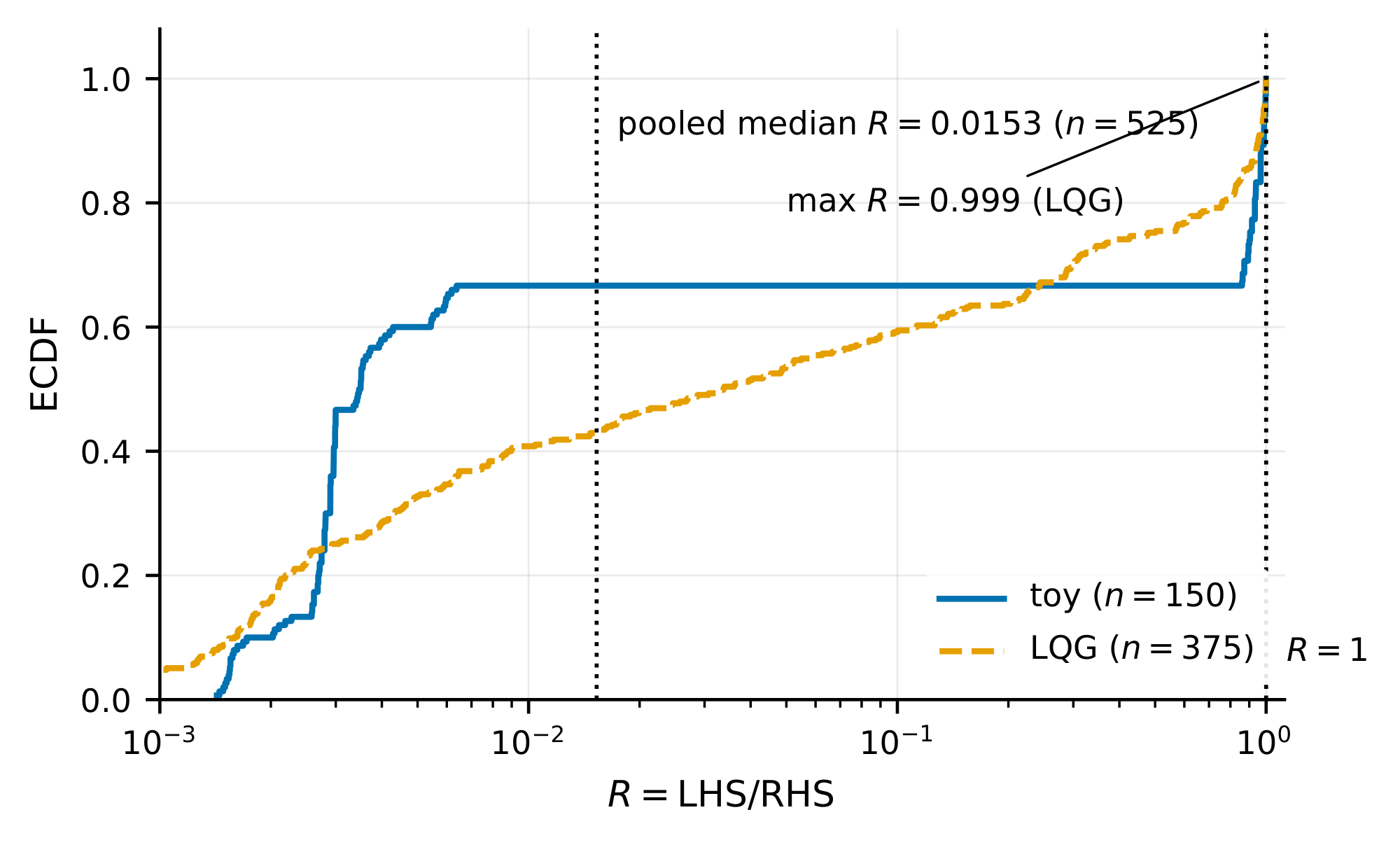
We empirically test the inequality in Equation 1. For each test configuration, define the realized return gap $\mathrm{LHS} := |J(\pi, \mathcal{M}) - J(\pi, \hat{\mathcal{M}})|$ and the bound's right-hand side $\mathrm{RHS} := (1-\gamma)^{-1}, \varepsilon_{\mathrm{rew}} + \frac{\gamma L_r(1+L_\pi)}{(1-\gamma)(1-\gamma L_f(1+L_\pi))}, \varepsilon_{\mathrm{dyn}}$, evaluated with the configuration's analytical Lipschitz constants $L_f, L_r, L_\pi$, discount factor $\gamma$, and realized per-step errors $\varepsilon_{\mathrm{dyn}}, \varepsilon_{\mathrm{rew}}$. We report the ratio $R := \mathrm{LHS}/\mathrm{RHS}$. The bound holds whenever $R \le 1$, and smaller $R$ indicates a looser bound. Each configuration consists of an $\textsc{mdp}$, an $L_\pi$-Lipschitz evaluation policy, and a perturbed model pair with realized per-step errors $\varepsilon_{\mathrm{dyn}}, \varepsilon_{\mathrm{rew}}$. We test on two benchmarks. The synthetic benchmark uses globally Lipschitz $f$ and $r$, so the hypotheses of Lemma 1 hold by construction. The Linear–Quadratic–Gaussian (LQG) benchmark uses a quadratic reward that is only locally Lipschitz, testing Lemma 1 on a bounded operating domain. Appendix B.4 describes the per-configuration construction. Across $n = 525$ configurations ($150$ synthetic, $375$ LQG) the bound holds on every configuration. The per-benchmark medians are $R^{\mathrm{med}}{\mathrm{synth}} = 0.0035$ and $R^{\mathrm{med}}{\mathrm{LQG}} = 0.034$, the pooled median is $0.015$, and the per-benchmark maxima are $R^{\max}{\mathrm{synth}} = 0.9995$ and $R^{\max}{\mathrm{LQG}} = 0.999$. For per-benchmark empirical CDF (ECDF) shapes and full implementation details, see Appendix B.4. Every configuration satisfies the bound, but the typical bound is loose: at the median it overshoots by $1/R^{\mathrm{med}}{\mathrm{LQG}} \approx 29\times$ on LQG and $1/R^{\mathrm{med}}{\mathrm{synth}} \approx 286\times$ on the synthetic benchmark (factor $\approx 65\times$ at the pooled median). Both benchmarks use deterministic dynamics; extending the calibration to stochastic dynamics or unbounded operating domains would require revisiting the assumptions of Lemma 1 and is left to future work.

4. The optimal sample allocation to minimize return error

Section Summary: To minimize long-term return error for a fixed sampling budget, one must optimally split resources between dynamics-transition samples, which teach a model how states evolve, and reward samples, which teach what payoffs each state-action pair produces. Both error types shrink according to fitted power laws as more data is collected, and the theory shows that the best ratio of the two sample types is proportional to their relative error rates, adjusted by per-sample costs and factors that capture how quickly small mistakes can compound over a planning horizon. Lower reward-sampling costs or shorter horizons therefore tilt the allocation toward more reward data, while cheaper dynamics data or longer horizons favor the opposite shift.

We distinguish between two types of samples: dynamics-transition samples and reward samples. A dynamics-transition sample $(s, a, f(s, a))$ consists of a state $s$, an action $a$, and the resulting next state $f(s, a)$. A reward sample $(s, a, r(s, a))$ consists of a state, an action, and the resulting reward $r(s, a)$. Let $N_{\mathrm{dyn}}$ and $N_{\mathrm{rew}}$ denote the numbers of dynamics-transition and reward samples, and let $c_{\mathrm{dyn}}$ and $c_{\mathrm{rew}}$ denote their per-sample costs. These costs may reflect any incurred costs, including environment interaction, annotation, and training on the samples. We reuse the symbols $\varepsilon_{\mathrm{dyn}}$ and $\varepsilon_{\mathrm{rew}}$ to denote the error levels achievable when the sample counts are $N_{\mathrm{dyn}}$ and $N_{\mathrm{rew}}$, according to standard power laws

$ \varepsilon_{dyn}(N_{dyn}) = A_d \cdot N_{dyn}^{-\alpha}, \qquad \varepsilon_{rew}(N_{rew}) = A_r \cdot N_{rew}^{-\beta}\tag{3} $

where $\alpha, \beta > 0$ are exponents fit from data, and $A_d, A_r$ are constants. For each budget $B = c_{\mathrm{dyn}} N_{\mathrm{dyn}} + c_{\mathrm{rew}} N_{\mathrm{rew}}$, let $(N_{\mathrm{dyn}}^*, N_{\mathrm{rew}}^*)$ denote a minimizer of the bound in Equation 1, and let $\varepsilon_{\mathrm{dyn}}^* := \varepsilon_{\mathrm{dyn}}(N_{\mathrm{dyn}}^*)$ and $\varepsilon_{\mathrm{rew}}^* := \varepsilon_{\mathrm{rew}}(N_{\mathrm{rew}}^*)$ be the dynamics and reward errors at those minimizing sample counts. We study the optimal ratio of dynamics samples to reward samples, $\frac{N_{\mathrm{dyn}}^*}{N_{\mathrm{rew}}^*}$, as $B \to \infty$.

########## {caption="Theorem 5: Optimal dynamics-to-reward sample ratio"}

If Equation 3 holds with exponents $\alpha, \beta > 0$ and the bound of Lemma 1 holds, then the minimizing sample counts $(N_{\mathrm{dyn}}^*, N_{\mathrm{rew}}^*)$ under the constraint $c_{\mathrm{dyn}} N_{\mathrm{dyn}} + c_{\mathrm{rew}} N_{\mathrm{rew}} = B$ satisfy

$ \frac{N_{dyn}^*}{N_{rew}^*} := \frac{\alpha}{\beta} \cdot \frac{\gamma L_r(1+L_\pi)}{1-\gamma L_f(1+L_\pi)} \cdot \frac{c_{rew}}{c_{dyn}} \cdot \frac{\varepsilon_{dyn}^*}{\varepsilon_{rew}^*}.\tag{4} $

Proof: See Appendix B.3.

Theorem 5 gives the optimal sample ratio $N_{\mathrm{dyn}}^*/N_{\mathrm{rew}}^*$ in terms of the error ratio $\varepsilon_{\mathrm{dyn}}^*/\varepsilon_{\mathrm{rew}}^*$, and shows that these two ratios are proportional. The multiplier in Equation 4 uses the global Lipschitz constants $L_f, L_r$ assumed by Lemma 1, so it is an upper bound rather than an equality. Section 4.2 measures, on the same configurations, how much smaller the realized value-function sensitivities are than these global constants, and how close the resulting prediction of $N_{\mathrm{dyn}}^*/N_{\mathrm{rew}}^*$ becomes. For practitioners who design systems that train policies in imagination, changes in sample costs or planning horizon affect the optimal sample ratio as follows.

Sample costs.

Costs enter through $c_{\mathrm{dyn}} N_{\mathrm{dyn}} + c_{\mathrm{rew}} N_{\mathrm{rew}} = B$ and the fitted error curves in Equation 3; in Equation 4, they appear as $c_{\mathrm{rew}}/c_{\mathrm{dyn}}$. Lowering $c_{\mathrm{rew}}$ lowers this factor, so $N_{\mathrm{dyn}}^*/N_{\mathrm{rew}}^*$ decreases and the allocation shifts toward reward samples. Lowering $c_{\mathrm{dyn}}$ raises the factor, so $N_{\mathrm{dyn}}^*/N_{\mathrm{rew}}^*$ increases and the allocation shifts toward dynamics-transition samples. However, since the optimal sample ratio also includes $\varepsilon_{\mathrm{dyn}}^*/\varepsilon_{\mathrm{rew}}^*$, these statements give the direction of the cost effect rather than a complete allocation rule by themselves.

Planning horizon.

The discounting effect is the familiar one: smaller $\gamma$ gives less weight to later rewards. As $\gamma$ decreases, Equation 1 becomes tighter, and the dynamics multiplier in Equation 4, $\gamma L_r(1+L_\pi)/(1-\gamma L_f(1+L_\pi))$, decreases. The optimal allocation therefore shifts toward reward samples, as expected for a shorter-horizon objective in which dynamics errors have fewer discounted steps to affect future rewards. A similar effect arises from lowering the Lipschitz constants of the learned models. By Corollary 2, lowering any of $L_f, L_r, L_\pi$ tightens Equation 1 and decreases the dynamics multiplier in Equation 4. The optimal allocation therefore shifts toward reward samples, since dynamics errors then compound less strongly along rollouts.

4.1 Numerical experiments: scaling of dynamics and reward errors

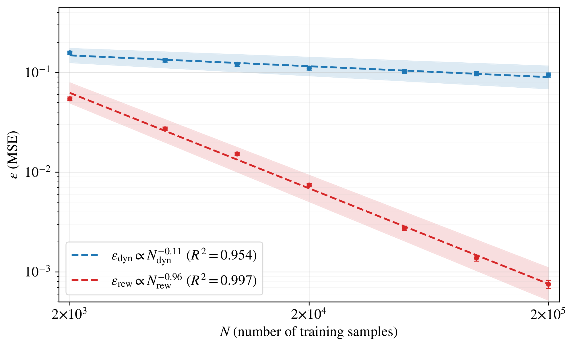
We estimate how fast each model learns with more data and whether the dynamics and reward models learn at the same rate. To this end, we conduct an experiment that tests the power-law scaling assumptions in Equation 3 and estimates the exponents $\alpha$ and $\beta$ for a particular architecture and environment. In this experiment, we estimate the dynamics and reward errors as a function of the number of training samples $N_{\mathrm{dyn}}$ and $N_{\mathrm{rew}}$, respectively, and fit the standard power-law scaling laws from Equation 3. Figure 1 shows the fitted scaling laws, which are consistent with the power-law assumptions in Theorem 5. It measures $\varepsilon_{\mathrm{dyn}}$ and $\varepsilon_{\mathrm{rew}}$ on a fixed held-out set $\mathcal{D}{\mathrm{val}}$ of transitions $(s, a, s', r)$ in a synthetic continuous-control environment whose dynamics and reward function are defined by frozen, randomly-initialized 2-layer ReLU MLPs, and whose students $\hat{f}$ and $\hat{r}$ use the same architecture as the teachers. Specifically, $\varepsilon{\mathrm{dyn}}(N_{\mathrm{dyn}}) := \frac{1}{|\mathcal{D}{\mathrm{val}}|} \sum{(s, a, s', r) \in \mathcal{D}{\mathrm{val}}} |\hat{f}(s, a) - s'|^2$ and $\varepsilon{\mathrm{rew}}(N_{\mathrm{rew}}) := \frac{1}{|\mathcal{D}{\mathrm{val}}|} \sum{(s, a, s', r) \in \mathcal{D}{\mathrm{val}}} (\hat{r}(s, a) - r)^2$, where $\hat{f}$ and $\hat{r}$ are trained on $N{\mathrm{dyn}}$ dynamics-transition samples and $N_{\mathrm{rew}}$ reward samples drawn independently of $\mathcal{D}{\mathrm{val}}$. We use $\varepsilon{\mathrm{dyn}}$ and $\varepsilon_{\mathrm{rew}}$ as practical surrogates for the sup-norm errors in Lemma 1. The fitted laws are $\varepsilon_{\mathrm{dyn}}(N_{\mathrm{dyn}}) = 0.34, N_{\mathrm{dyn}}^{-0.11}$ with $R^2 = 0.954$ and $\varepsilon_{\mathrm{rew}}(N_{\mathrm{rew}}) = 90.4, N_{\mathrm{rew}}^{-0.96}$ with $R^2 = 0.997$. For bootstrap standard errors, 95% bootstrap confidence intervals, and full implementation details, see Appendix C.2. The exponent ratio $0.96 / 0.11 \approx 9$ is the central empirical observation: reward error decays nearly an order of magnitude faster per decade of training data than dynamics error. This ratio of exponents is consistent with $\hat{r}$ predicting a scalar while $\hat{f}$ predicts a $d_s$-dimensional next state, and its exact value depends on the dimensions and architectures used here.

4.2 Empirical evaluation of Equation 4

Equation 4 predicts $N_{\mathrm{dyn}}^*/N_{\mathrm{rew}}^*$ as the product of two factors: the proportionality $N_{\mathrm{dyn}}^*/N_{\mathrm{rew}}^* \propto \varepsilon_{\mathrm{dyn}}^*/\varepsilon_{\mathrm{rew}}^*$ and a multiplier that depends on $\gamma$, $L_f$, $L_r$, $L_\pi$, $c_{\mathrm{rew}}/c_{\mathrm{dyn}}$, and $\alpha/\beta$. We test the two factors separately: whether the proportionality holds when the multiplier is replaced by realized value-function sensitivities, and how loose the multiplier is when instantiated with the global Lipschitz constants assumed by Lemma 1. Define the log-ratio residual $\ell := \log(N_{\mathrm{dyn}}^*/N_{\mathrm{rew}}^*) - \log(\varepsilon_{\mathrm{dyn}}^*/\varepsilon_{\mathrm{rew}}^*)$, so $|\ell| \le \log 3$ means predicted and realized ratios agree within a factor of $3$. The realized value-function sensitivities $S_f, S_r$ and the per-configuration construction are defined in Appendix B.5. Replacing the global constants $L_f, L_r$ with the realized sensitivities $S_f, S_r$ recovers the predicted ratio. We test this recovery on configurations whose value function $V^\pi$ has a known parametric form: linear, $\tanh$, $\sin$, and a separate quadratic-value control group that isolates the looseness from using $\sup$-norm overestimates in place of the realized sensitivities. The linear configurations achieve median $|\ell| = 0$ and Spearman rank correlation $\rho = 1$ between predicted and realized ratios; this case is an algebraic consistency check rather than an empirical test, since a linear $V^\pi$ forces the realized sensitivities to match the analytical ratio. The empirical content comes from the nonlinear configurations: $\tanh$ and $\sin$ give median $|\ell| = 0.054$. On the control group, substituting $\sup$-norm overestimates for the realized sensitivities inflates the median residual by roughly an order of magnitude. Figure 2 plots predicted against realized sample ratios $N_{\mathrm{dyn}}^*/N_{\mathrm{rew}}^*$ for each group. Instantiating the multiplier with the analytical global Lipschitz constants of Lemma 1, by contrast, overshoots realized ratios by about three orders of magnitude. On the LQG configurations every configuration's $\ell$ is positive, with median $\ell = 7.585$ (a factor $\exp(7.585) \approx 1968$ between predicted and realized ratios). Figure 4 shows the per-configuration distribution of $\ell$. The contraction regime, sample sizes, statistical methodology, and a separate ratio isolating the dynamics-coefficient contribution to the multiplier are reported in Appendix B.5.

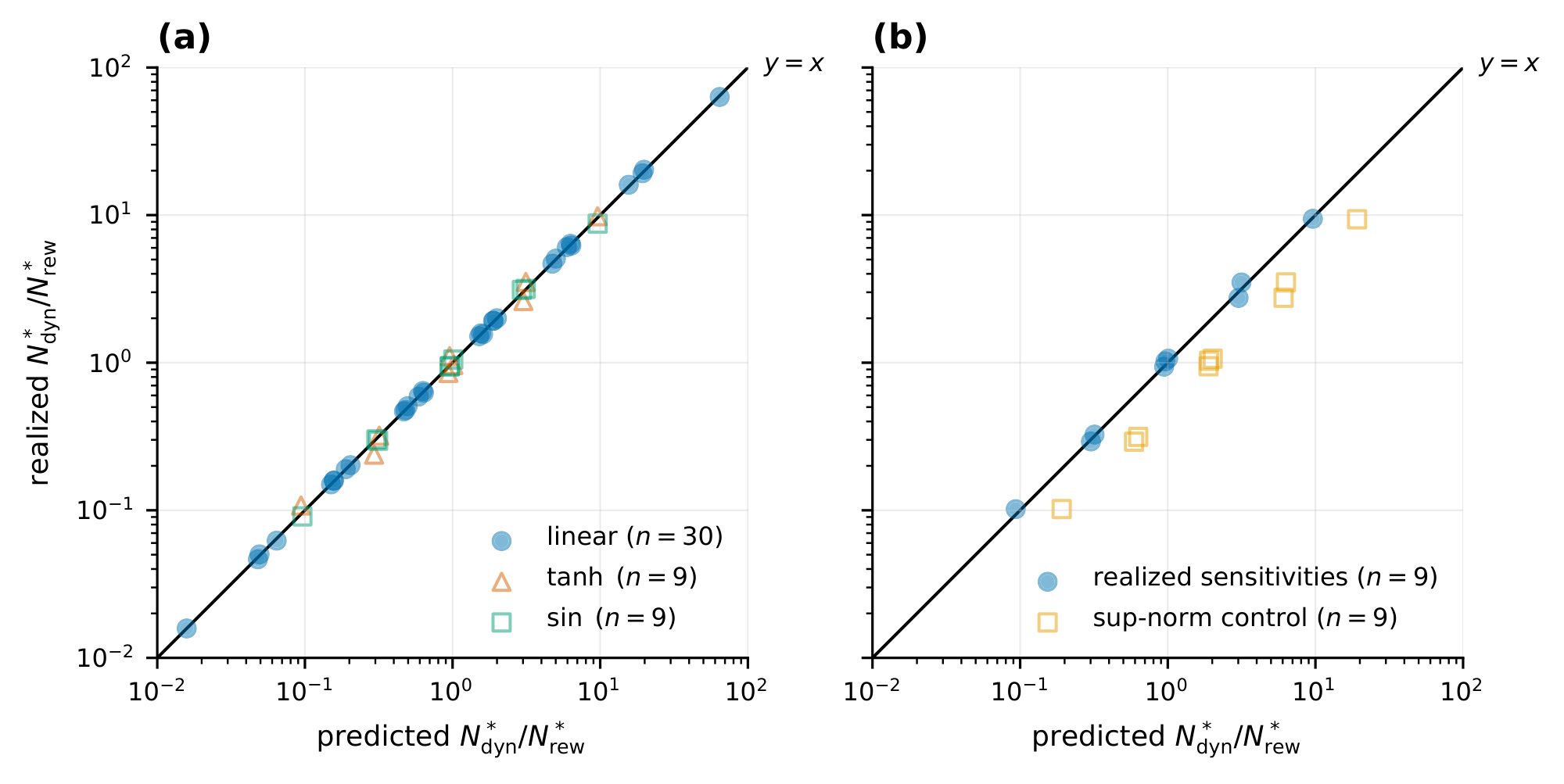
The proportionality $N_{\mathrm{dyn}}^*/N_{\mathrm{rew}}^* \propto \varepsilon_{\mathrm{dyn}}^*/\varepsilon_{\mathrm{rew}}^*$ in Equation 4 therefore carries the predictive content, while the multiplier built from global Lipschitz constants is loose at the order-of-magnitude scale. Recovering the predicted ratio requires evaluating $V^\pi$ at perturbed models (the construction in Appendix B.5), which may be impractical at scale.

5. Cost-effective learning from noisy rewards

Section Summary: The section examines policy-gradient learning with the REINFORCE estimator when observed rewards contain additive zero-mean noise. It shows that the estimator remains unbiased, yet the noise adds an extra term to the gradient variance that grows with the noise level and shrinks with more sampled trajectories. For a fixed annotation budget the authors reduce the fidelity-versus-quantity tradeoff to minimizing a simple function Φ(c) = c · noise-variance(c), and they illustrate how different relationships between cost and noise (such as power laws) determine whether one should buy many cheap noisy labels or a few high-quality ones.

The reward-noise analysis in this section is independent of the allocation results in Section 4: the unbiasedness statement for $\textsc{reinforce}$ under zero-mean reward noise applies to any stationary MDP satisfying the standard policy-gradient assumptions, regardless of how dynamics and reward samples are allocated.

We study policy optimization under noisy rewards through the classical $\textsc{reinforce}$ estimator introduced by [12]. In this section let $\pi_\theta$ be a differentiable policy, fix a finite horizon $H$, and fix a discount factor $\gamma \in [0, 1)$. Define $J_H(\pi, \mathcal{M}) := \mathbb{E}[\sum_{t=0}^{H-1} \gamma^t r(s_t, a_t)]$, where the expectation is over trajectories generated by executing $\pi$ in $\mathcal{M}$. Define the discounted cumulative reward from time $t$ onward as $G_t := \sum_{t'=t}^{H-1} \gamma^{t'-t} r(s_{t'}, a_{t'})$, so that $G_0$ is the discounted return of the full trajectory and $J_H(\pi, \mathcal{M}) = \mathbb{E}[G_0]$. Define the finite-horizon policy gradient by $g_H := \nabla_\theta J_H(\pi_\theta, \mathcal{M})$. Define the noisy counterpart of $G_t$ as $\hat{G}t := \sum{t'=t}^{H-1} \gamma^{t'-t}\hat{r}{t'}$, where $\hat{r}t$ denotes the observed reward at time $t$. The $\textsc{reinforce}$ estimator of $g_H$ computed from a single trajectory is $\hat{g}^{(1)} := \sum{t=0}^{H-1} \nabla\theta \log \pi_\theta(a_t \mid s_t), \hat{G}t$. To estimate $g_H$, sample $K \geq 1$ independent trajectories by executing $\pi\theta$ in $\mathcal{M}$. For each $k \in {1, \ldots, K}$, let $\hat{g}^{(k)}$ denote the $\textsc{reinforce}$ estimator computed on the $k$ th trajectory, and define $\hat{g} := \frac{1}{K}\sum_{k=1}^K \hat{g}^{(k)}$. The estimators $\hat{g}^{(1)}, \ldots, \hat{g}^{(K)}$, $\hat{g}$, and their noise-free counterparts are vector-valued. To measure their dispersion with a single scalar, we use the natural generalization of scalar variance obtained by adding coordinate variances: for $z=(z_1, \ldots, z_d)$, write $\mathrm{Var}[z] := \sum_{i=1}^d \mathrm{Var}[z_i]$.

########## {caption="Theorem 6: Finite-horizon reinforce under noisy rewards"}

Assume $W_H^2 := \mathbb{E}\bigl[\max_{0 \leq t \leq H-1}|\nabla_\theta \log \pi_\theta(a_t \mid s_t)|^2\bigr] < \infty$. Suppose the rewards are observed with additive noise, $\hat{r}t = r(s_t, a_t) + \eta_t$, where the noise variables $\eta_t$ are i.i.d. with $\mathbb{E}[\eta_t] = 0$ and $\mathrm{Var}[\eta_t] = \sigma\eta^2 < \infty$, and each $\eta_t$ is independent of the state-action history $((s_0, a_0), \ldots, (s_t, a_t))$. Then $\hat{g}$ satisfies

$ \mathbb{E}[\hat{g}] = g_H, \qquad Var[\hat{g}] \leq Var[\hat{g}] _{\eta \equiv 0}

• \frac{\sigma_\eta^2 H W_H^2}{K(1-\gamma)^2}. $

where $\mathrm{Var}[\hat{g}] _{\eta \equiv 0}$ denotes the variance of the same estimator when the rewards are noise-free.

Proof: See Appendix B.6.

In many settings, practitioners can pay more per reward annotation to obtain less noisy rewards, for example by averaging multiple annotators or using a more careful annotation pipeline. We use Theorem 6 to ask how a fixed budget for reward annotations should be split between fidelity (lower noise per annotation) and quantity (more rollouts at higher noise).

Let $c > 0$ denote the per-rollout cost of acquiring reward annotations along that rollout, and define $\sigma_\eta^2(c) := \mathrm{Var}[\eta_t \mid \text{per-rollout annotation cost equals } c] \in [0, \infty)$ as the variance of the reward noise $\eta_t$ from Theorem 6 when reward annotations are acquired at per-rollout cost $c$. We assume that $\sigma_\eta^2 \colon (0, \infty) \to [0, \infty)$ is measurable. Given a budget $B > 0$ for reward annotations, the number of independent rollouts that fit in the budget at fidelity $c$ is $K = B/c$.

########## {caption="Corollary 7: Optimal fidelity for noise-induced variance"}

Define $\Phi(c) := c, \sigma_\eta^2(c)$. Under the assumptions of Theorem 6 with $\mathrm{Var}[\eta_t] = \sigma_\eta^2(c)$ and $K = B/c$, the upper bound on the noise-induced excess variance from Theorem 6 equals $\Phi(c), H, W_H^2 / (B, (1-\gamma)^2)$. Consequently, any $c^* \in \operatorname*arg, min_{c > 0} \Phi(c)$ minimizes this upper bound over $c > 0$.

Proof: Substituting $K = B/c$ into the upper bound from Theorem 6 gives $\sigma_\eta^2(c), H, W_H^2 / (K, (1-\gamma)^2) = \Phi(c), H, W_H^2 / (B, (1-\gamma)^2)$. The prefactor $H, W_H^2 / (B, (1-\gamma)^2)$ is non-negative and does not depend on $c$, so the upper bound and $\Phi(c)$ share their minimizers over $c > 0$.

Corollary 7 reduces the choice of fidelity for reward annotations to minimizing $\Phi(c)$. We illustrate the consequences with three examples of how the noise variance $\sigma_\eta^2(c)$ depends on the cost $c$, summarized in Figure 5.

Power-law fidelity.

Suppose $\sigma_\eta^2(c) = A, c^{-p}$ for constants $A, p > 0$, so that each multiplicative increase in cost yields a fixed multiplicative reduction in noise variance. Then $\Phi(c) = A, c^{1-p}$, which is strictly decreasing in $c$ when $p > 1$, strictly increasing in $c$ when $p < 1$, and constant when $p = 1$. The exponent $p = 1$ therefore separates two regimes: when $p > 1$, the bound is minimized by paying for the highest-fidelity annotations available; when $p < 1$, the bound is minimized by paying as little as possible per annotation and using the saved budget for additional rollouts.

Bounded fidelity.

Suppose $\sigma_\eta^2(c) = \sigma_0^2, (1 - c/c_{\max})$ on $(0, c_{\max}]$ for constants $\sigma_0^2, c_{\max} > 0$, modeling a setting in which annotations have variance $\sigma_0^2$ as $c \to 0$ and become noise-free at the finite cost $c_{\max}$. Then $\Phi(c) = \sigma_0^2, c, (1 - c/c_{\max})$ is a downward parabola in $c$ that is maximized at $c = c_{\max}/2$, attains the value $0$ at $c = c_{\max}$, and approaches $0$ as $c \to 0$. Both extremes of the cost range therefore minimize the bound, and intermediate fidelities are strictly worse.

Irreducible noise floor.

Suppose $\sigma_\eta^2(c) = \sigma_{\mathrm{floor}}^2 + A/c$ for constants $\sigma_{\mathrm{floor}}^2, A > 0$, modeling a setting in which no level of spending can drive the noise variance below $\sigma_{\mathrm{floor}}^2$. Then $\Phi(c) = \sigma_{\mathrm{floor}}^2, c + A$ is strictly increasing in $c$, so the bound is minimized by $c \to 0$: when reward noise has a floor that money cannot remove, the optimal allocation buys the cheapest annotations and relies on the $1/K$ factor in Theorem 6 to reduce variance.

Together, these cases show that the shape of $\Phi(c)$ determines whether the budget should be spent on fidelity, on quantity, or on one of the two extremes.

The preceding results assume the reward noise is zero-mean. We note that this assumption is essential: averaging over more trajectories cannot remove a systematic reward bias.

########## {caption="Proposition 8: Finite-horizon reinforce under biased rewards"}

Let $b:\mathcal{S}\times\mathcal{A}\to\mathbb{R}$ be a reward bias function, define $\tilde{r}(s, a) := r(s, a) + b(s, a)$, and define $\tilde{\mathcal{M}} := (\mathcal{S}, \mathcal{A}, f, \tilde{r}, \gamma)$. For trajectories sampled by executing $\pi_\theta$ under the true dynamics $f$, let $\tilde{g}^{(1)}, \ldots, \tilde{g}^{(K)}$ be independent $\textsc{reinforce}$ estimators computed using the biased rewards $\tilde{r}(s_t, a_t)$, and define $\tilde{g} := \frac{1}{K}\sum_{k=1}^K \tilde{g}^{(k)}$. Define $B_H(\theta) := \mathbb{E}!\left[\sum_{t=0}^{H-1}\gamma^t b(s_t, a_t)\right]$, where the expectation is over trajectories generated by executing $\pi_\theta$ under the true dynamics $f$. Then

$ \mathbb{E}[\tilde{g}] = \nabla_\theta J_H(\pi_\theta, \tilde{\mathcal{M}}) = g_H + \nabla_\theta B_H(\theta).\tag{5} $

If $\mathrm{Var}[\tilde{g}^{(1)}] < \infty$, then

$ \mathbb{E}!\left[|\tilde{g}-g_H|^2\right] = \frac{1}{K}Var[\tilde{g}^{(1)}]

• |\nabla_\theta B_H(\theta)|^2.\tag{6} $

Consequently, when $\nabla_\theta B_H(\theta) \neq 0$, averaging over more trajectories reduces the variance term but does not remove the bias as an estimator of $g_H$.

Proof: See Appendix B.8.

6. Discussion

Section Summary: The model defines next states and rewards using only the current state and chosen action. This setup does not force the environment to forget earlier events or observations. Instead, any relevant history can be folded into the present state itself, for instance by letting a recurrent neural network maintain a running summary of what has occurred so far.

Although the dynamics $f:\mathcal{S}\times\mathcal{A}\to\mathcal{S}$ and reward $r:\mathcal{S}\times\mathcal{A}\to\mathbb{R}$ depend only on the current state and action, this does not require the underlying environment to be memoryless: any dependence on past states and actions can be absorbed into $\mathcal{S}$ by taking the state to encode a summary of the past, e.g. via recurrent neural networks ([18, 19, 20, 21]).

7. Acknowledgments

Section Summary: The acknowledgments section recognizes the financial support that enabled the authors' research. Nadav Timor credits GitHub for Startups and Lambda AI for their help, while Micah Goldblum notes funding from Dream Sports along with a Google Research Award. David Harel was supported by a grant from Magnus Konow given in memory of his mother, Olga Konow Rappaport.

Nadav Timor thanks GitHub for Startups and Lambda AI for generous financial support. Micah Goldblum was supported by Dream Sports and the Google Research Award. David Harel was supported by a research grant from Magnus Konow in honour of his mother Olga Konow Rappaport.

Appendix

Section Summary: This appendix gathers supplementary background research that supports the paper's overall framework without directly supporting its central technical contributions. It reviews prior studies on latent world models for training agents in simulation, error bounds for approximate planning, methods for allocating limited simulation resources, policy gradient analysis, and techniques for learning stable representations. The section then supplies the full mathematical proofs, beginning with a detailed inductive argument establishing trajectory error bounds for Lemma 1 under Lipschitz continuity assumptions on the dynamics and policy.

A. Additional related work

This appendix collects related works that inform the setting of Section 2 but are not load-bearing for the novelty claims of Lemma 1, Theorem 5, Theorem 6, Corollary 7, Proposition 8, Corollary 2, and Proposition 4.

Latent-state world models.

Beyond the works cited in Section 2, several lines of work shape the modern training-in-imagination paradigm. [22] fit a Gaussian-process dynamics model and propagate uncertainty through imagined trajectories under a known reward. [23] learn a latent dynamics model from pixels and train a policy primarily inside this learned model. Dreamer ([24]) learns a latent-space dynamics model together with a learned reward predictor and optimizes the policy entirely on imagined latent rollouts. [5] learn a value-equivalent latent model whose dynamics, reward, and value predictions are trained jointly to support planning, and [25] combine a learned latent dynamics and reward model with short-horizon planning and a learned terminal value.

Simulation-style bounds and value-aware model learning.

The simulation-lemma family extends in several directions. [26] express the difference in expected discounted return between two policies as an expectation of single-step advantages under one of them, which underpins conservative policy iteration. [27] gives $L_p$-style error-propagation bounds for approximate policy iteration, and [28] recently establish optimal tightness for the simulation lemma. A parallel line of work asks whether the model loss should target value prediction rather than raw transition accuracy: value-aware model learning ([29]) replaces the next-state likelihood objective with a loss measuring the worst-case discrepancy between the true and learned dynamics on expected values over a class of value functions, [30] show that, restricted to a 1-Lipschitz value-function class, this loss is equivalent to the Wasserstein distance between the dynamics, and [31] addresses how to learn the reward function on states drawn from a misspecified dynamics model.

Active observation and simulation budget allocation.

Active-measure reinforcement learning chooses when to pay for an observation under explicit observation costs ([32]). In the simulation-optimization literature, optimal computing budget allocation divides a fixed simulation budget across candidate policies to maximize the probability of selecting the best one ([33]). Power-law fits analogous to those of [10] and [11] have since been reported for single-agent reinforcement learning and for pre-training of agents and world models ([34, 35]).

Policy-gradient theory and reward modeling.

Beyond [12], the policy-gradient theorem of [36] and the variance-reduction analysis of [37] provide the standard analytic toolkit invoked by Theorem 6. [38] characterize how the $\textsc{reinforce}$ noise-to-signal ratio varies non-uniformly across the parameter landscape. Reinforcement learning from human feedback trains reward models from preferences ([39, 40]), the empirical setting in which [15] document Goodhart-style overoptimization.

Representation learning and Lipschitz regularization.

[41] provide a concrete image instantiation of joint-embedding predictive architectures, and [42] propose projection-based mechanisms for enforcing Lipschitz continuity during training, with upper bounds applicable to multiple $p$-norms beyond the spectral norm.

B. Full proofs

B.1 Proof of Lemma 1

Proof: Fix an $L_\pi$-Lipschitz policy $\pi$ and a shared initial state $s_0 = \hat{s}_0$. Let ${s_t}$ denote the state trajectory generated by executing $\pi$ under the true dynamics $f$, and ${\hat{s}_t}$ the trajectory under $\hat{f}$, both starting from $s_0$. The actions differ because the policy is evaluated at different states:

$ a_t = \pi(s_t), \qquad \hat{a}_t = \pi(\hat{s}_t). $

At each step $t$:

$ \begin{aligned} r(s_t, a_t) - \hat{r}(\hat{s}_t, \hat{a}_t) &= \bigl[r(s_t, a_t) - r(\hat{s}_t, \hat{a}_t)\bigr]

• \bigl[r(\hat{s}_t, \hat{a}_t) - \hat{r}(\hat{s}_t, \hat{a}_t)\bigr]. \end{aligned}\tag{7} $

Let $L_{\mathrm{comp}} := L_f(1 + L_\pi)$. By induction:

$ |s_t - \hat{s}t| \leq \varepsilon{dyn} \sum_{k=0}^{t-1} L_{comp}^k $

Base case ($t=0$): $s_0 = \hat{s}_0$, so $|s_0 - \hat{s}_0| = 0$.

Inductive step: Assume $|s_t - \hat{s}t| \leq \varepsilon{\mathrm{dyn}} \sum_{k=0}^{t-1} L_{\mathrm{comp}}^k$.

$ \begin{aligned} |s_{t+1} - \hat{s}{t+1}| &= |f(s_t, a_t) - \hat{f}(\hat{s}t, \hat{a}t)| \notag \ &\leq |f(s_t, a_t) - f(\hat{s}t, \hat{a}t)| + |f(\hat{s}t, \hat{a}t) - \hat{f}(\hat{s}t, \hat{a}t)| \notag \ &\leq L_f\bigl(|s_t - \hat{s}t| + |a_t - \hat{a}t|\bigr) + \varepsilon{dyn} \notag \ &= L_f\bigl(|s_t - \hat{s}t| + |\pi(s_t) - \pi(\hat{s}t)|\bigr) + \varepsilon{dyn} \notag \ &\leq L_f\bigl(|s_t - \hat{s}t| + L\pi|s_t - \hat{s}t|\bigr) + \varepsilon{dyn} \notag \ &\leq L_f(1 + L\pi)|s_t - \hat{s}t| + \varepsilon{dyn} \notag \ &= L{comp}|s_t - \hat{s}t| + \varepsilon{dyn} \notag \ &\leq L{comp}\left(\varepsilon{dyn} \sum{k=0}^{t-1} L{comp}^k\right) + \varepsilon{dyn} \notag \ &= \varepsilon{dyn} \sum{k=0}^{t-1} L{comp}^{k+1} + \varepsilon{dyn} \notag \ &= \varepsilon_{dyn} \sum_{k=0}^{t-1} L_{comp}^{k+1} + \varepsilon_{dyn} L_{comp}^0 \notag \ &= \varepsilon_{dyn} \sum_{j=1}^{t} L_{comp}^j + \varepsilon_{dyn} L_{comp}^0 \notag \ &= \varepsilon_{dyn} \sum_{k=0}^{t} L_{comp}^k. \notag \end{aligned} $

Error from using the learned reward function: $|r(\hat{s}_t, \hat{a}_t) - \hat{r}(\hat{s}t, \hat{a}t)| \leq \varepsilon{\mathrm{rew}}$, by the definition of $\varepsilon{\mathrm{rew}}$.

Error from evaluating the true reward at different state-action pairs:

$ \begin{aligned} |r(s_t, a_t) - r(\hat{s}_t, \hat{a}_t)| &\leq L_r\bigl(|s_t - \hat{s}_t| + |a_t - \hat{a}t|\bigr) \notag \ &= L_r\bigl(|s_t - \hat{s}t| + |\pi(s_t) - \pi(\hat{s}t)|\bigr) \notag \ &\leq L_r\bigl(|s_t - \hat{s}t| + L\pi|s_t - \hat{s}t|\bigr) \notag \ &= L_r(1 + L\pi)|s_t - \hat{s}t| \notag \ &\leq L_r(1+L\pi) \varepsilon{dyn} \sum{k=0}^{t-1} L{comp}^k. \notag \end{aligned} $

Using the definition of discounted return and 7,

$ \begin{aligned} |J(\pi, \mathcal{M}) - J(\pi, \hat{\mathcal{M}})| &= \left|\sum_{t=0}^{\infty} \gamma^t \bigl(r(s_t, a_t) - \hat{r}(\hat{s}_t, \hat{a}t)\bigr)\right| \notag \ &\leq \sum{t=0}^{\infty} \gamma^t \left|r(s_t, a_t) - \hat{r}(\hat{s}_t, \hat{a}t)\right| \notag \ &= \sum{t=0}^{\infty} \gamma^t \left|\bigl(r(s_t, a_t) - r(\hat{s}_t, \hat{a}_t)\bigr)

• \bigl(r(\hat{s}_t, \hat{a}_t) - \hat{r}(\hat{s}_t, \hat{a}t)\bigr)\right| \notag \ &\leq \sum{t=0}^{\infty} \gamma^t \left|r(s_t, a_t) - r(\hat{s}_t, \hat{a}_t)\right|
• \sum_{t=0}^{\infty} \gamma^t \left|r(\hat{s}t, \hat{a}t) - \hat{r}(\hat{s}t, \hat{a}t)\right| \notag \ &\leq L_r(1+L\pi) \varepsilon{dyn} \sum{t=0}^{\infty} \gamma^t \left(\sum{k=0}^{t-1} L_{comp}^k\right)
• \varepsilon_{rew} \sum_{t=0}^{\infty} \gamma^t \notag \ &= L_r(1+L_\pi) \varepsilon_{dyn} \sum_{t=0}^{\infty}\sum_{k=0}^{t-1} \gamma^t L_{comp}^k
• \frac{1}{1 - \gamma}, \varepsilon_{rew} \notag \ &= L_r(1+L_\pi) \varepsilon_{dyn} \sum_{k=0}^{\infty} \sum_{\substack{t=0 \ k \le t-1}}^{\infty} \gamma^t L_{comp}^k
• \frac{1}{1 - \gamma}, \varepsilon_{rew} \notag \ &= L_r(1+L_\pi) \varepsilon_{dyn} \sum_{k=0}^{\infty} \sum_{t=k+1}^{\infty} \gamma^t L_{comp}^k
• \frac{1}{1 - \gamma}, \varepsilon_{rew} \notag \ &= L_r(1+L_\pi) \varepsilon_{dyn} \sum_{k=0}^{\infty} \sum_{j=0}^{\infty} \gamma^{k+1+j}L_{comp}^k
• \frac{1}{1 - \gamma}, \varepsilon_{rew} \notag \ &= L_r(1+L_\pi) \varepsilon_{dyn} \sum_{k=0}^{\infty} \left(\gamma^{k+1}\sum_{j=0}^{\infty} \gamma^j\right)L_{comp}^k
• \frac{1}{1 - \gamma}, \varepsilon_{rew} \notag \ &= \frac{\gamma L_r(1+L_\pi)}{1-\gamma}, \varepsilon_{dyn} \sum_{k=0}^{\infty} (\gamma L_{comp})^k
• \frac{1}{1 - \gamma}, \varepsilon_{rew} \notag \ \end{aligned} $

$Because \gamma L_{comp} < 1, the geometric series converges.$

$ \begin{aligned} &= \frac{\gamma L_r(1+L_\pi)}{1-\gamma}, \varepsilon_{dyn} \left(\frac{1}{1-\gamma L_{comp}}\right)

• \frac{1}{1 - \gamma}, \varepsilon_{rew} \notag \ &= \frac{1}{1 - \gamma}, \varepsilon_{rew} + \frac{\gamma L_r(1+L_\pi)}{(1-\gamma)(1-\gamma L_f(1+L_\pi))}, \varepsilon_{dyn} \notag \end{aligned} $

B.2 Proof of Proposition 4

Proof: Fix $t$ such that $v(z_t)\neq 0$ and $v(z_{t+1})\neq 0$, and set

$ a:=v(z_t), \qquad b:=v(z_{t+1}). $

Along the rollout, $a=z_{t+1}-z_t$ and $b=z_{t+2}-z_{t+1}$. Using the $\varepsilon$-Lipschitz condition for $v$ gives

$ \begin{aligned} |b-a| &= |v(z_{t+1})-v(z_t)| \ &\leq \varepsilon|z_{t+1}-z_t| \ &= \varepsilon|a|. \end{aligned} $

By the triangle inequality,

$ \begin{aligned} |b| &= |a+(b-a)| \ &\geq |a|-|b-a| \ &\geq (1-\varepsilon)|a|. \end{aligned} $

Define

$ C := \frac{a^\top b}{|a||b|}. $

Then

$ \begin{aligned} |b-a|^2 &= |a|^2+|b|^2-2a^\top b \ &= |a|^2+|b|^2-2C|a||b| \ &= (|a|-|b|)^2 + 2|a||b|(1-C). \end{aligned} $

Rearranging and using $(|a|-|b|)^2\geq 0$ yields

$ \begin{aligned} 1-C &= \frac{|b-a|^2-(|a|-|b|)^2}{2|a||b|} \ &\leq \frac{|b-a|^2}{2|a||b|}. \end{aligned} $

Substituting $|b-a|\leq \varepsilon|a|$ and $|b|\geq (1-\varepsilon)|a|$ gives

$ \begin{aligned} 1-C &\leq \frac{\varepsilon^2|a|^2}{2|a|(1-\varepsilon)|a|} \ &= \frac{\varepsilon^2}{2(1-\varepsilon)}. \end{aligned} $

Since $1-C=\mathcal{L}_{\mathrm{curv}}(t)$ by definition, this proves the curvature-loss bound.

The function $\varepsilon \mapsto \varepsilon^2/(2(1-\varepsilon))$ is increasing on $(0, 1)$ because

$ \frac{d}{d\varepsilon}\frac{\varepsilon^2}{2(1-\varepsilon)} = \frac{\varepsilon(2-\varepsilon)}{2(1-\varepsilon)^2}>0. $

Therefore lowering the Lipschitz constant of $v$ lowers the upper bound whenever the Lipschitz constant remains in $(0, 1)$.

B.3 Proof of Theorem 5

Proof: For sample counts $(N_{\mathrm{dyn}}, N_{\mathrm{rew}})$, Equation 3 gives

$ \varepsilon_{rew}(N_{rew}) = A_r N_{rew}^{-\beta}, \qquad \varepsilon_{dyn}(N_{dyn}) = A_d N_{dyn}^{-\alpha}. $

Substituting these identities into the upper bound from Equation 1 gives

$ \frac{A_r}{1-\gamma}, N_{rew}^{-\beta}

• \frac{\gamma L_r(1+L_\pi)}{(1-\gamma)(1-\gamma L_f(1+L_\pi))}, A_d, N_{dyn}^{-\alpha}. $

Define the sample-count-independent coefficients by

$ C_r := \frac{A_r}{1-\gamma}, \qquad C_d := \frac{\gamma L_r(1+L_\pi) A_d}{(1-\gamma)(1-\gamma L_f(1+L_\pi))}, $

so the upper bound after substitution becomes

$ \mathcal{L}{bound}(N{dyn}, N_{rew}) := C_r N_{rew}^{-\beta} + C_d N_{dyn}^{-\alpha}. $

For the fixed budget $B$, the feasible sample counts are exactly the pairs $(N_{\mathrm{dyn}}, N_{\mathrm{rew}})$ satisfying $c_{\mathrm{dyn}} N_{\mathrm{dyn}} + c_{\mathrm{rew}} N_{\mathrm{rew}} = B$. Therefore minimizing the upper bound from Equation 1 over all feasible sample counts is equivalent to minimizing $\mathcal{L}{\mathrm{bound}}(N{\mathrm{dyn}}, N_{\mathrm{rew}})$ subject to the same budget constraint.

Because $\alpha, \beta > 0$, the objective decreases as either sample count increases, so the minimizer satisfies $N_{\mathrm{dyn}}^* > 0$ and $N_{\mathrm{rew}}^* > 0$. Define the Lagrangian

$ \Lambda(N_{dyn}, N_{rew}, \lambda) := C_d N_{dyn}^{-\alpha} + C_r N_{rew}^{-\beta}

• \lambda(c_{dyn} N_{dyn} + c_{rew} N_{rew} - B). $

Because the minimizing counts satisfy $N_{\mathrm{dyn}}^* > 0$ and $N_{\mathrm{rew}}^* > 0$, setting the partial derivatives of $\Lambda$ with respect to $N_{\mathrm{dyn}}$ and $N_{\mathrm{rew}}$ equal to zero gives

$ \begin{aligned} \alpha, C_d, N_{dyn}^{-\alpha - 1} &= \lambda, c_{dyn}, \ \beta, C_r, N_{rew}^{-\beta - 1} &= \lambda, c_{rew}. \end{aligned} $

Multiply the equation for $N_{\mathrm{dyn}}$ by $N_{\mathrm{dyn}}$ and the equation for $N_{\mathrm{rew}}$ by $N_{\mathrm{rew}}$:

$ \begin{aligned} \alpha, C_d, N_{dyn}^{-\alpha} &= \lambda, c_{dyn} N_{dyn}, \ \beta, C_r, N_{rew}^{-\beta} &= \lambda, c_{rew} N_{rew}. \end{aligned} $

Now divide the equation for $N_{\mathrm{dyn}}$ by the equation for $N_{\mathrm{rew}}$:

$ \begin{aligned} \frac{\alpha, C_d, N_{dyn}^{-\alpha}}{\beta, C_r, N_{rew}^{-\beta}} &= \frac{c_{dyn} N_{dyn}}{c_{rew} N_{rew}}. \end{aligned} $

Rearranging this identity gives

$ \frac{N_{dyn}}{N_{rew}} = \frac{\alpha}{\beta} \cdot \frac{c_{rew}}{c_{dyn}} \cdot \frac{C_d N_{dyn}^{-\alpha}}{C_r N_{rew}^{-\beta}}.\tag{8} $

Evaluate Equation 8 at the minimizing counts $(N_{\mathrm{dyn}}^*, N_{\mathrm{rew}}^*)$. Using the definition of $C_d$ together with Equation 3, we obtain

$ \begin{aligned} C_d (N_{dyn}^*)^{-\alpha} &= \frac{\gamma L_r(1+L_\pi)}{(1-\gamma)(1-\gamma L_f(1+L_\pi))}, A_d (N_{dyn}^*)^{-\alpha} \ &= \frac{\gamma L_r(1+L_\pi)}{(1-\gamma)(1-\gamma L_f(1+L_\pi))}, \varepsilon_{dyn}^*, \ C_r (N_{rew}^*)^{-\beta} &= \frac{A_r}{1-\gamma} (N_{rew}^*)^{-\beta} \ &= \frac{1}{1-\gamma}, \varepsilon_{rew}^*. \end{aligned} $

Substituting these two identities yields

$ \begin{aligned} \frac{N_{dyn}^*}{N_{rew}^*} &= \frac{\alpha}{\beta} \cdot (1-\gamma)\frac{\gamma L_r(1+L_\pi)}{(1-\gamma)(1-\gamma L_f(1+L_\pi))} \cdot \frac{c_{rew}}{c_{dyn}} \cdot \frac{\varepsilon_{dyn}^*}{\varepsilon_{rew}^*} \ &= \frac{\alpha}{\beta} \cdot \frac{\gamma L_r(1+L_\pi)}{1-\gamma L_f(1+L_\pi)} \cdot \frac{c_{rew}}{c_{dyn}} \cdot \frac{\varepsilon_{dyn}^*}{\varepsilon_{rew}^*}. \end{aligned} $

Because $x \mapsto x^{-\alpha}$ and $x \mapsto x^{-\beta}$ are convex on $(0, \infty)$ for $\alpha, \beta > 0$, the objective is convex on the feasible set. Therefore the feasible point satisfying the derivative equations for $N_{\mathrm{dyn}}$ and $N_{\mathrm{rew}}$ is the unique minimizer.

B.4 Experiment details: empirical calibration of the decomposed bound

This appendix collects the protocol and per-configuration construction for the calibration experiment in Section 3.1, whose main-text result is summarized in Figure 3.

Each configuration is a tuple $(f, r, \pi, \hat{f}, \hat{r})$, where $(f, r)$ is an $\textsc{mdp}$ instance, $\pi$ is an $L_\pi$-Lipschitz evaluation policy, and $(\hat{f}, \hat{r})$ is the perturbed model pair. The realized per-step errors $\varepsilon_{\mathrm{dyn}}, \varepsilon_{\mathrm{rew}}$ are computed from the $(f, \hat{f})$ and $(r, \hat{r})$ pair using the same definitions that the main-text formulas use.

The synthetic benchmark contains $n = 150$ configurations in which $f$ and $r$ are globally Lipschitz; on this benchmark $L_f, L_r, L_\pi$ in $\mathrm{RHS}$ of Equation 1 are computed analytically as the global Lipschitz constants of the configuration's maps. The LQG benchmark contains $n = 375$ configurations in which the quadratic reward is Lipschitz only on a bounded operating domain (a fixed compact subset of state-action space within which the configuration's rollouts are confined); on this benchmark $L_r$ is the Lipschitz constant of $r$ restricted to that domain.

The empirical CDFs of $R$ in Figure 3 have qualitatively different shapes on the two benchmarks. The LQG ECDF climbs steadily across $R \in [10^{-3}, 1]$. The synthetic ECDF rises sharply through its low- $R$ mass, stays flat at value $\approx 0.66$ across $R \in [10^{-2}, , 5\times 10^{-1}]$, and then climbs toward $R = 1$ on the remaining $\approx 25%$ of configurations. The pooled median $R = 0.015$ is therefore dominated by the LQG arm. The pool maximum is $R = 0.9995$ on a synthetic configuration, and the LQG arm peaks at $R = 0.999$.

Two annotations on Figure 3 should be read as follows: $\texttt{maxR = 0.999(LQG)}$ is the LQG-arm maximum (the pool maximum is the slightly larger synthetic value $R = 0.9995$), and the legend label toy denotes the synthetic benchmark.

We report only the per-benchmark medians, the pooled median, and the per-benchmark maxima; no bootstrap confidence intervals are used because the relevant claim is the universal $R \le 1$, which is verified directly on every configuration.

B.5 Experiment details: empirical evaluation of the optimal sample-ratio formula

This appendix collects the per-configuration construction, definitions, statistical methodology, and numerical results for the allocation-evaluation experiment in Section 4.2, whose main-text findings are summarized in Figure 2 and Figure 4.

The configurations used in Figure 2 and Figure 4 are partitioned into four groups, each generated by a Cartesian product over a small set of axes; per-configuration values are recorded in the committed CSVs and we list the grids verbatim below. The interpretation of the axes sigma_ratio, cost_ratio, $\lambda$, and theta_f0 is deferred to the open item at the end of this appendix.

Linear-value configurations ($n = 30$, panel (a) of Figure 2).

The Cartesian product is $(L_f, \lambda) \in {(0.5, 0.5), ; (2.0, 2.0)}$ (with $L_f = \lambda$ enforced) crossed with $\texttt{sigma_ratio} \in {0.1, 0.3, 1.0, 3.0, 10.0}$ and $\texttt{cost_ratio} \in {0.1, 1.0, 10.0}$, for $2 \times 5 \times 3 = 30$ configurations. The reward Lipschitz constant is fixed at $L_r = 1$.

$\tanh$-value and $\sin$-value configurations ($n = 9$ each, panel (a) of Figure 2).

For each of these two value-function families, the Cartesian product is $\texttt{sigma_ratio} \in {0.3, 1.0, 3.0}$ crossed with $\texttt{cost_ratio} \in {0.1, 1.0, 10.0}$, with $L_f = L_r = \lambda = 1$ fixed.

Quadratic-value $\sup$-norm-control configurations ($n = 9$, panel (b) of Figure 2).

The Cartesian product is the same $\texttt{sigma_ratio} \times \texttt{cost_ratio}$ grid of size $9$, with $\lambda = 1$ and $\texttt{theta_f0} = 0.5$ fixed. Each configuration is evaluated twice: once with $L_f^{\mathrm{local}} = 1$ (the realized-sensitivity calculation, plotted as filled circles in panel (b)) and once with $L_f^{\sup} = 2$ (the $\sup$-norm control, plotted as open squares).

LQG configurations ($n = 30$, Figure 4).

Configurations are indexed by $\texttt{seed} \in {0, 1, \ldots, 29}$ and parameterized so that, at $\gamma = 0.8$, the contraction quantity $\gamma L_f (1 + L_\pi)$ lies in $[0.224, 0.228]$ (margin $1 - \gamma L_f (1 + L_\pi) \in [0.772, 0.776]$). The realized constants per seed land in $L_f \in [0.280, 0.285]$, $L_\pi \in [1.6\times 10^{-4}, 1.0\times 10^{-3}]$, $L_r \in [0.82, 1.49]$.

For each seed we fit per-configuration power-law scaling laws $\varepsilon_{\mathrm{dyn}}(N) = A_d \cdot N^{-\alpha_d}$ and $\varepsilon_{\mathrm{rew}}(N) = A_r \cdot N^{-\alpha_r}$, with $A_d \in [1.0\times 10^{-3}, 1.7\times 10^{-3}]$, $A_r \in [2.2\times 10^{-3}, 4.0\times 10^{-3}]$, $\alpha_d \in [0.97, 1.05]$, $\alpha_r \in [0.99, 1.08]$, $R^2_d \in [0.995, 0.9997]$, and $R^2_r \in [0.996, 0.9998]$ (recorded per-configuration in the A_d, A_r, alpha_d, alpha_r, R2_d, R2_r columns of lqg_per_instance.csv). These per-seed exponents are distinct from the global $\alpha, \beta$ fit in Section 4.1.

The boundary_excluded column reports that $0/30$ configurations were filtered out as boundary cases (the filter would exclude any configuration whose realized contraction $\gamma L_f(1+L_\pi)$ approached $1$, which would invalidate the hypothesis of Lemma 1; none did).

We define the quantities used in this experiment. Let $V^\pi(s; f, r)$ denote the discounted return of a fixed evaluation policy $\pi$ when the dynamics map is $f$ and the reward map is $r$. For each test configuration, let $\Delta f := \hat{f} - f$ and $\Delta r := \hat{r} - r$ denote the realized model perturbations, and fix a step size $h>0$. Define the realized value sensitivities by the one-sided finite-difference quotients

$ \begin{aligned} S_f(s, a) &;:=; \frac{|V^\pi(s; f + h, \Delta f, r) - V^\pi(s; f, r)|}{h, |\Delta f|}, \ S_r(s, a) &;:=; \frac{|V^\pi(s; f, r + h, \Delta r) - V^\pi(s; f, r)|}{h, |\Delta r|}, \end{aligned} $

where $|\cdot|$ is the Euclidean norm; as $h \to 0$, $S_f$ and $S_r$ approach the directional derivatives $\partial_f V^\pi$ and $\partial_r V^\pi$, which provide the underlying intuition for these realized sensitivities. The global Lipschitz constant of the dynamics map in the spectral norm is any

$ L_f ;\geq; \sup_{(s, a)\neq(s', a')}; \frac{|f(s, a) - f(s', a')|}{|s-s'| + |a-a'|}, $

and $L_r$ is defined analogously, on a bounded operating domain when the reward is only locally Lipschitz. Let $K_{\mathrm{Lip}} := \frac{\gamma L_r(1+L_\pi)}{(1-\gamma)(1-\gamma L_f(1+L_\pi))}$ denote the dynamics coefficient appearing in Equation 1, instantiated with the analytical global Lipschitz constants $L_f, L_r$, and let $K'$ denote the same coefficient with $L_f$ in the contraction factor $1 - \gamma L_f(1+L_\pi)$ replaced by the realized value-function sensitivity $S_f$. The log-ratio residual $\ell$ is defined in Section 4.2.

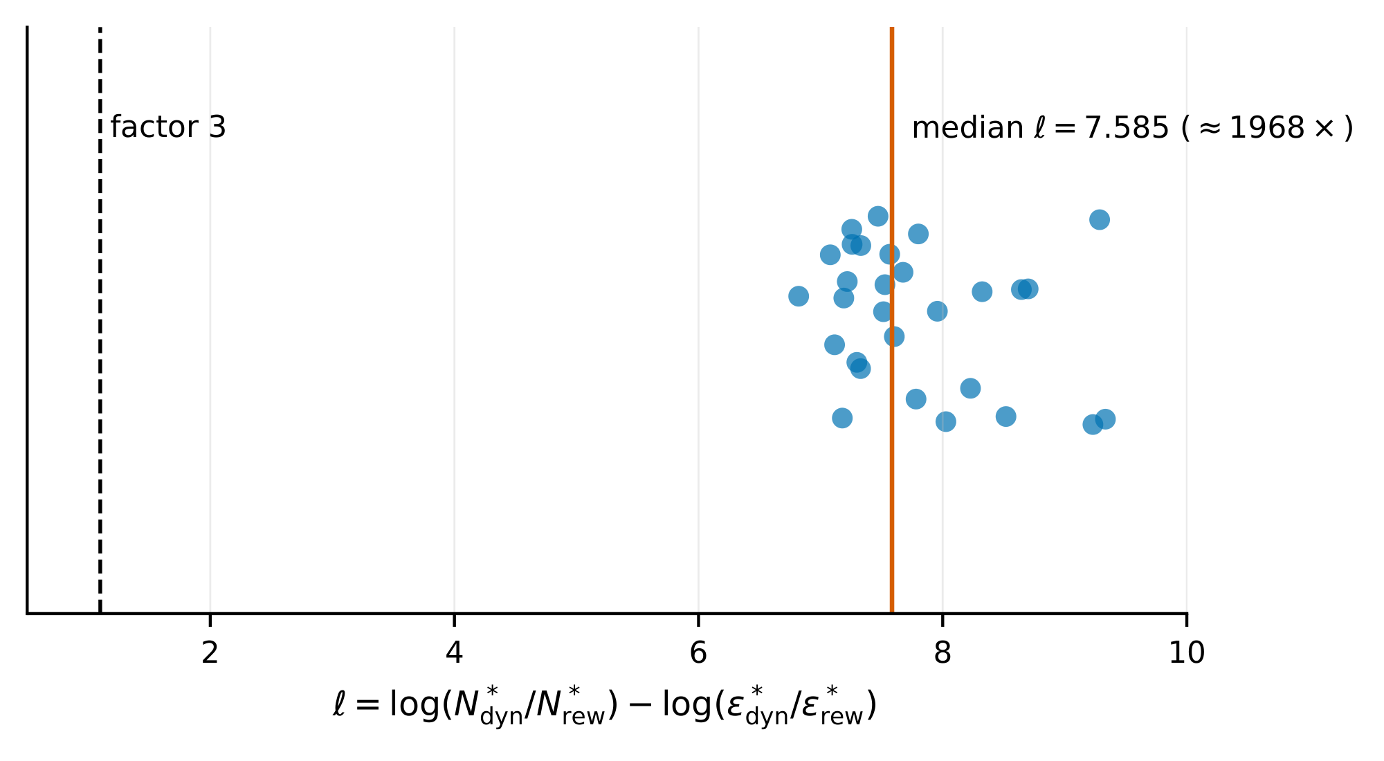
We summarize each group of configurations by the across-configuration median of $|\ell|$ (or $\ell$ when overshoot direction is informative); Figure 4 jitters the vertical position of each LQG marker for visibility. To check that overshoot in the global-Lipschitz multiplier comparison is not consistent with chance, we run a one-sided sign test against the null that overprediction and underprediction are equally likely; with $30/30$ configurations overshooting, the test gives $p = 0.5^{30} \approx 9.31 \times 10^{-10}$.

The headline per-group medians are reported in Section 4.2; here we record the additional numbers underlying the $\sup$-norm-control comparison. On the $9$ quadratic-value configurations, the median residual rises from $|\ell_{\mathrm{realized}}| = 0.074$ to $|\ell_{\sup}| = 0.684$ when realized sensitivities are replaced by their $\sup$-norm overestimates, a factor of $\approx 9.25\times$. The maximum $|\ell|$ on the linear-value configurations is also $0$, complementing the median value of $0$ already reported in main text.

A separate statistic isolates the dynamics-coefficient slack itself. On the same $n = 30$ LQG configurations (committed per-configuration as the K_prime column of lqg_per_instance.csv), the multiplier ratio $K_{\mathrm{Lip}} / K'$ has median $2.37$ and maximum $3.23$ (minimum $1.71$). This is a different quantity from the residual $\ell$: the factor $\approx 1968$ figure is $\exp(7.585)$ on the residual itself, while $K_{\mathrm{Lip}} / K'$ isolates the contribution of replacing the global $L_f$ with the realized $S_f$ in the dynamics-side coefficient alone.

Worst-case bounds in approximate dynamic programming, such as the simulation-lemma bounds on policy-evaluation and policy-improvement error stated in terms of model error, are classically conservative when instantiated with global Lipschitz or sup-norm constants ([27, 26]). The pattern observed here matches that classical observation: the bound in Lemma 1 certifies a sufficient condition, while the proportionality in Equation 4 carries the predictive content for sample allocation.

B.6 Proof of Theorem 6

Proof: A trajectory $\tau = ((s_0, a_0), \ldots, (s_{H-1}, a_{H-1}))$ is sampled by executing $\pi_\theta$ in $\mathcal{M}$. Let $G_t$, $\hat{G}t$, and $\hat{g}^{(1)}$ be as defined in Section 5. Define the corresponding $\textsc{reinforce}$ estimator when the rewards are noise-free as $g^{(1)} := \sum{t=0}^{H-1} \nabla_\theta \log \pi_\theta(a_t \mid s_t), G_t$, so $\mathbb{E}_{\tau}[g^{(1)}] = g_H$.

Let $N_t := \sum_{t'=t}^{H-1} \gamma^{t'-t} \eta_{t'}$, so that $\hat{G}t = G_t + N_t$. Let $\delta^{(1)} := \sum{t=0}^{H-1} \nabla_\theta \log \pi_\theta(a_t \mid s_t), N_t$, so that $\hat{g}^{(1)} = g^{(1)} + \delta^{(1)}$. Fix the sampled trajectory $\tau$ and take conditional expectation over the reward noise. Because each $\eta_{t'}$ is independent of the state-action history and has mean zero,

$ \begin{aligned} \mathbb{E}[N_t \mid \tau] &= \sum_{t'=t}^{H-1} \gamma^{t'-t}, \mathbb{E}[\eta_{t'} \mid \tau] \ &= \sum_{t'=t}^{H-1} \gamma^{t'-t}, \mathbb{E}[\eta_{t'}] \ &= 0. \end{aligned} $

Therefore

$ \begin{aligned} \mathbb{E}[\delta^{(1)} \mid \tau] &= \sum_{t=0}^{H-1} \nabla_\theta \log \pi_\theta(a_t \mid s_t), \mathbb{E}[N_t \mid \tau] \ &= 0, \end{aligned}\tag{9} $

and hence

$ \mathbb{E}[\hat{g}^{(1)} \mid \tau] = g^{(1)}. $

Therefore $\mathbb{E}[\hat{g}^{(1)}] = \mathbb{E}[g^{(1)}] = g_H$, and averaging over $K$ trajectories gives $\mathbb{E}[\hat{g}] = g_H$.

Fix the sampled trajectory $\tau$ and define

$ w_t := \nabla_\theta \log \pi_\theta(a_t \mid s_t). $

Then

$ \begin{aligned} \delta^{(1)} &= \sum_{t=0}^{H-1} w_t \sum_{t'=t}^{H-1} \gamma^{t'-t}\eta_{t'} \ &= \sum_{t=0}^{H-1} \sum_{t'=t}^{H-1} \gamma^{t'-t} w_t \eta_{t'} \ &= \sum_{t'=0}^{H-1} \sum_{\substack{t=0 \ t \le t'}}^{H-1} \gamma^{t'-t} w_t \eta_{t'} \ &= \sum_{t'=0}^{H-1} \sum_{t=0}^{t'} \gamma^{t'-t} w_t \eta_{t'}. \end{aligned} $

Define

$ v_{t'} := \sum_{t=0}^{t'} \gamma^{t'-t} w_t. $

Then

$ \delta^{(1)} = \sum_{t'=0}^{H-1} v_{t'} \eta_{t'}. $

Using Equation 9,

$ \begin{aligned} Var[\delta^{(1)} \mid \tau] &= \sum_{i=1}^d Var[\delta^{(1)}i \mid \tau] \ &= \sum{i=1}^d \mathbb{E}!\left[\left(\delta^{(1)}i-\mathbb{E}[\delta^{(1)}i \mid \tau]\right)^2 \middle| \tau\right] \ &= \mathbb{E}\bigl[|\delta^{(1)} - \mathbb{E}[\delta^{(1)} \mid \tau]|^2 \mid \tau\bigr] \ &= \mathbb{E}\bigl[|\delta^{(1)}|^2 \mid \tau\bigr] \ &= \mathbb{E}!\left[\left|\sum{t'=0}^{H-1} v{t'} \eta_{t'}\right|^2 \middle| \tau\right] \ &= \mathbb{E}!\left[\left\langle \sum_{t'=0}^{H-1} v_{t'} \eta_{t'}, \sum_{u=0}^{H-1} v_u \eta_u \right\rangle \middle| \tau\right] \ &= \mathbb{E}!\left[\sum_{t'=0}^{H-1} \sum_{u=0}^{H-1} \left\langle v_{t'} \eta_{t'}, v_u \eta_u \right\rangle \middle| \tau\right] \ &= \mathbb{E}!\left[\sum_{t'=0}^{H-1} \sum_{u=0}^{H-1} \eta_{t'}\eta_u \langle v_{t'}, v_u\rangle \middle| \tau\right] \ &= \sum_{t'=0}^{H-1} \sum_{u=0}^{H-1} \mathbb{E}[\eta_{t'}\eta_u \mid \tau] , \langle v_{t'}, v_u\rangle \ &= \sum_{t'=0}^{H-1} \mathbb{E}[\eta_{t'}^2 \mid \tau] , \langle v_{t'}, v_{t'}\rangle + \sum_{t'=0}^{H-1} \sum_{\substack{u=0 \ u \neq t'}}^{H-1} \mathbb{E}[\eta_{t'}\eta_u \mid \tau] , \langle v_{t'}, v_u\rangle \ \end{aligned} $

For t' \neq u, independence of the reward noise from \tau, together with independence across time and zero mean, gives \mathbb{E}[\eta_{t'}\eta_u \mid \tau] = \mathbb{E}[\eta_{t'}\eta_u] = \mathbb{E}[\eta_{t'}]\mathbb{E}[\eta_u] = 0, while \mathbb{E}[\eta_{t'}^2 \mid \tau] = \mathbb{E}[\eta_{t'}^2] = \sigma_\eta^2. Therefore

$ \begin{aligned} &= \sum_{t'=0}^{H-1} \sigma_\eta^2 |v_{t'}|^2 \ &= \sigma_\eta^2 \sum_{t'=0}^{H-1} |v_{t'}|^2. \end{aligned} $

Next,

$ \begin{aligned} |v_{t'}| &= \left|\sum_{t=0}^{t'} \gamma^{t'-t} w_t\right| \ &\leq \sum_{t=0}^{t'} \gamma^{t'-t}|w_t| \ &\leq \left(\sum_{t=0}^{t'} \gamma^{t'-t}\right) \max_{0 \leq t \leq H-1}|w_t| \ &\leq \frac{1}{1-\gamma}\max_{0 \leq t \leq H-1}|w_t|. \end{aligned} $

Substituting the bound on $|v_{t'}|$ into the conditional variance gives

$ \begin{aligned} Var[\delta^{(1)} \mid \tau] &\leq \sigma_\eta^2 \sum_{t'=0}^{H-1} \left(\frac{1}{1-\gamma}\max_{0 \leq t \leq H-1}|w_t|\right)^2 \ &= \frac{\sigma_\eta^2 H}{(1-\gamma)^2} \max_{0 \leq t \leq H-1}|w_t|^2. \end{aligned} $

Taking expectations over $\tau$ and using the definitions of $w_t$ and $W_H^2$ yields

$ \begin{aligned} \mathbb{E}[Var[\delta^{(1)}|\tau]] &\leq \frac{\sigma_\eta^2 H}{(1-\gamma)^2} \mathbb{E}!\left[\max_{0 \leq t \leq H-1}|w_t|^2\right] \ &= \frac{\sigma_\eta^2 H}{(1-\gamma)^2} \mathbb{E}!\left[\max_{0 \leq t \leq H-1} |\nabla_\theta \log \pi_\theta(a_t \mid s_t)|^2\right] \ &= \frac{\sigma_\eta^2 H W_H^2}{(1-\gamma)^2}. \end{aligned} $

Now apply the law of total variance to each coordinate and sum over coordinates. Here the conditional variance is over the reward noise given a fixed trajectory $\tau$:

$ \begin{aligned} Var[\hat{g}^{(1)}] &= Var!\bigl(\mathbb{E}[\hat{g}^{(1)} \mid \tau]\bigr)

• \mathbb{E}\bigl[Var[\hat{g}^{(1)} \mid \tau]\bigr] \notag \ &= Var[g^{(1)}]
• \mathbb{E}\bigl[Var[g^{(1)} + \delta^{(1)} \mid \tau]\bigr] \notag \ \end{aligned} $

$Because g^{(1)} depends only on \tau, conditioning on \tau makes g^{(1)} deterministic. Hence Var[g^{(1)} + \delta^{(1)} \mid \tau] = Var[\delta^{(1)} \mid \tau] almost surely, so$

$ \begin{aligned} &= Var[g^{(1)}] + \mathbb{E}[Var[\delta^{(1)} \mid \tau]] \notag \ &\leq Var[g^{(1)}]

• \frac{\sigma_\eta^2 H W_H^2}{(1-\gamma)^2}. \end{aligned}\tag{10} $

Since the trajectories and their reward noises are sampled independently across $k$, the estimators $\hat{g}^{(1)}, \ldots, \hat{g}^{(K)}$ are independent. Each estimator has mean $g_H$. Write $\hat{g}_i$ and $(g_H)_i$ for the $i$ th coordinates of $\hat{g}$ and $g_H$. Then

$ \begin{aligned} Var[\hat{g}] &= \sum_{i=1}^d Var[\hat{g}i] \notag \ &= \sum{i=1}^d \mathbb{E}!\left[(\hat{g}i-\mathbb{E}[\hat{g}i])^2\right] \notag \ &= \sum{i=1}^d \mathbb{E}!\left[(\hat{g}i-(g_H)i)^2\right] \notag \ &= \mathbb{E}!\left[\sum{i=1}^d(\hat{g}i-(g_H)i)^2\right] \notag \ &= \mathbb{E}!\left[|\hat{g}-g_H|^2\right] \notag \ &= \mathbb{E}!\left[\left|\frac{1}{K}\sum{k=1}^K \hat{g}^{(k)}-g_H\right|^2\right] \notag \ &= \frac{1}{K^2}\mathbb{E}!\left[\left|\sum{k=1}^K(\hat{g}^{(k)}-g_H)\right|^2\right] \notag \ &= \frac{1}{K^2}\mathbb{E}!\left[\left\langle \sum{k=1}^K(\hat{g}^{(k)}-g_H), \sum{\ell=1}^K(\hat{g}^{(\ell)}-g_H) \right\rangle \right] \notag \ &= \frac{1}{K^2}\sum_{k=1}^K \sum_{\ell=1}^K \mathbb{E}!\left[\left\langle \hat{g}^{(k)}-g_H, \hat{g}^{(\ell)}-g_H \right\rangle \right] \notag \ \end{aligned} $

$For k \neq \ell, independence gives \mathbb{E}[\langle \hat{g}^{(k)}-g_H, \hat{g}^{(\ell)}-g_H\rangle] = \langle \mathbb{E}[\hat{g}^{(k)}-g_H], \mathbb{E}[\hat{g}^{(\ell)}-g_H]\rangle = 0. Therefore only the terms with k = \ell remain, so$

$ \begin{aligned} &= \frac{1}{K^2}\sum_{k=1}^K \mathbb{E}!\left[\left\langle \hat{g}^{(k)}-g_H, \hat{g}^{(k)}-g_H \right\rangle \right] \notag \ &= \frac{1}{K^2}\sum_{k=1}^K \mathbb{E}!\left[\sum_{i=1}^d(\hat{g}^{(k)}i-(g_H)i)^2\right] \notag \ &= \frac{1}{K^2}\sum{k=1}^K \sum{i=1}^d \mathbb{E}!\left[(\hat{g}^{(k)}_i-(g_H)_i)^2\right] \notag \ \end{aligned} $

$Since each coordinate of \hat{g}^{(k)} has mean the corresponding coordinate of g_H, $

$ \begin{aligned} &= \frac{1}{K^2}\sum_{k=1}^K \sum_{i=1}^d Var[\hat{g}^{(k)}_i] \notag \ \end{aligned} $

$By the definition of Var for vector-valued estimators, $

$ \begin{aligned} &= \frac{1}{K^2}\sum_{k=1}^K Var[\hat{g}^{(k)}] \notag \ \end{aligned} $

$The estimators \hat{g}^{(1)}, \ldots, \hat{g}^{(K)} have the same distribution, so each term in the sum equals Var[\hat{g}^{(1)}]:$

$ \begin{aligned} &= \frac{1}{K^2}\sum_{k=1}^K Var[\hat{g}^{(1)}] \notag \ &= \frac{1}{K}Var[\hat{g}^{(1)}]. \end{aligned}\tag{11} $

When the rewards are noise-free, the averaged estimator $\hat{g}$ equals $\hat{g} = \frac{1}{K}\sum_{k=1}^K g^{(k)}$. Repeating the expansion above gives

$ \begin{aligned} Var[\hat{g}] {\eta \equiv 0} &= Var!\left[\frac{1}{K}\sum{k=1}^K g^{(k)}\right] \notag \ &= \frac{1}{K^2}\sum_{k=1}^K \sum_{\ell=1}^K \mathbb{E}!\left[\left\langle g^{(k)}-g_H, g^{(\ell)}-g_H \right\rangle \right] \notag \ \end{aligned} $

$For k \neq \ell, independence gives \mathbb{E}[\langle g^{(k)}-g_H, g^{(\ell)}-g_H\rangle] = \langle \mathbb{E}[g^{(k)}-g_H], \mathbb{E}[g^{(\ell)}-g_H]\rangle = 0, so$

$ \begin{aligned} &= \frac{1}{K^2}\sum_{k=1}^K \mathbb{E}!\left[|g^{(k)}-g_H|^2\right] \notag \ &= \frac{1}{K^2}\sum_{k=1}^K Var[g^{(k)}] \notag \ &= \frac{1}{K^2}\sum_{k=1}^K Var[g^{(1)}] \notag \ &= \frac{1}{K}Var[g^{(1)}]. \end{aligned}\tag{12} $

Combining Equation 11 with Equation 10 gives

$ \begin{aligned} Var[\hat{g}] &= \frac{1}{K}Var[\hat{g}^{(1)}] \ &\leq \frac{1}{K}\left(Var[g^{(1)}]

• \frac{\sigma_\eta^2 H W_H^2}{(1-\gamma)^2}\right) \ &= \frac{1}{K}Var[g^{(1)}]
• \frac{\sigma_\eta^2 H W_H^2}{K(1-\gamma)^2} \ &= Var[\hat{g}] _{\eta \equiv 0}
• \frac{\sigma_\eta^2 H W_H^2}{K(1-\gamma)^2}, \end{aligned} $

where the last equality uses Equation 12.

B.7 Visualization of the three fidelity-cost regimes from Corollary 7

Figure 5 plots $\sigma_\eta^2(c)$ and $\Phi(c) = c, \sigma_\eta^2(c)$ for the three regimes analyzed in Section 5.

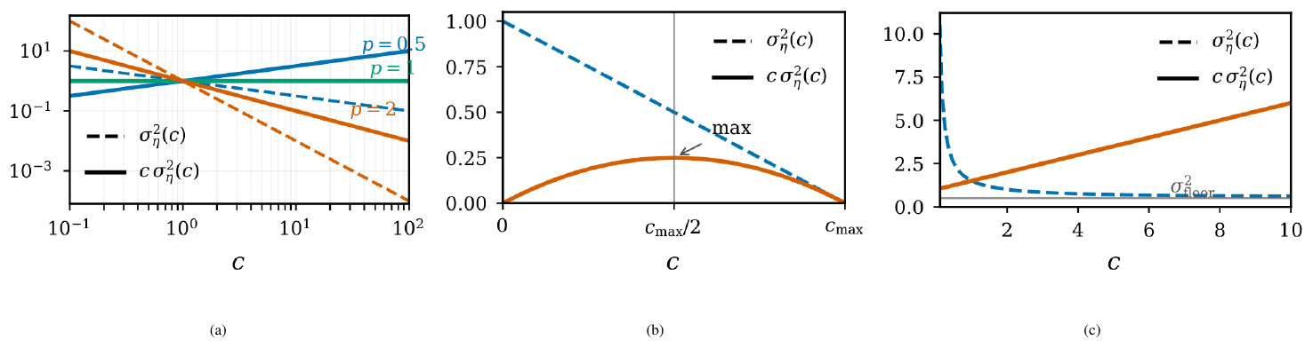
B.8 Proof of Proposition 8

Proof: For one trajectory $\tau = ((s_0, a_0), \ldots, (s_{H-1}, a_{H-1}))$ sampled by executing $\pi_\theta$ under the true dynamics $f$, define the biased finite-horizon return from time $t$ onward by

$ \tilde{G}t := \sum{t'=t}^{H-1}\gamma^{t'-t}\tilde{r}(s_{t'}, a_{t'}). $

The single-trajectory estimator using biased rewards is

$ \tilde{g}^{(1)} := \sum_{t=0}^{H-1} \nabla_\theta \log \pi_\theta(a_t \mid s_t), \tilde{G}_t. $

The estimator $\tilde{g}^{(1)}$ is the finite-horizon $\textsc{reinforce}$ estimator for the $\textsc{mdp}$ $\tilde{\mathcal{M}}$, which has the true dynamics $f$ and the biased reward $\tilde{r}$. Therefore the finite-horizon policy-gradient identity gives

$ \mathbb{E}[\tilde{g}^{(1)}] = \nabla_\theta J_H(\pi_\theta, \tilde{\mathcal{M}}). $

Averaging over $K$ independent trajectories does not change the mean:

$ \begin{aligned} \mathbb{E}[\tilde{g}] &= \mathbb{E}!\left[\frac{1}{K}\sum_{k=1}^K \tilde{g}^{(k)}\right] \ &= \frac{1}{K}\sum_{k=1}^K \mathbb{E}[\tilde{g}^{(k)}] \ &= \nabla_\theta J_H(\pi_\theta, \tilde{\mathcal{M}}). \end{aligned} $

By the definitions of $\tilde{r}$, $J_H$, and $B_H$,

$ \begin{aligned} J_H(\pi_\theta, \tilde{\mathcal{M}}) &= \mathbb{E}!\left[\sum_{t=0}^{H-1}\gamma^t \tilde{r}(s_t, a_t)\right] \ &= \mathbb{E}!\left[\sum_{t=0}^{H-1}\gamma^t (r(s_t, a_t) + b(s_t, a_t))\right] \ &= \mathbb{E}!\left[\sum_{t=0}^{H-1}\gamma^t r(s_t, a_t)\right]

• \mathbb{E}!\left[\sum_{t=0}^{H-1}\gamma^t b(s_t, a_t)\right] \ &= J_H(\pi_\theta, \mathcal{M}) + B_H(\theta). \end{aligned} $

Taking gradients with respect to $\theta$ gives

$ \begin{aligned} \nabla_\theta J_H(\pi_\theta, \tilde{\mathcal{M}}) &= \nabla_\theta J_H(\pi_\theta, \mathcal{M})

• \nabla_\theta B_H(\theta) \ &= g_H + \nabla_\theta B_H(\theta). \end{aligned} $

Combining the preceding displays proves Equation 5.

Let

$ \mu_b := \mathbb{E}[\tilde{g}] - g_H. $

By Equation 5, $\mu_b = \nabla_\theta B_H(\theta)$. We use the identity $|x+y|^2=|x|^2+2\langle x, y\rangle+|y|^2$ with $x=\tilde{g}-\mathbb{E}[\tilde{g}]$ and $y=\mu_b$. We also use linearity of expectation and the fact that $\mu_b$ is a fixed vector once $\theta$ is fixed, so $\mathbb{E}[|\mu_b|^2]=|\mu_b|^2$. Then

$ \begin{aligned} \mathbb{E}!\left[|\tilde{g}-g_H|^2\right] &= \mathbb{E}!\left[|\tilde{g}-\mathbb{E}[\tilde{g}] + \mathbb{E}[\tilde{g}]-g_H|^2 \right] \ &= \mathbb{E}!\left[|\tilde{g}-\mathbb{E}[\tilde{g}] + \mu_b|^2 \right] \ &= \mathbb{E}!\left[|\tilde{g}-\mathbb{E}[\tilde{g}]|^2

• 2\left\langle \tilde{g}-\mathbb{E}[\tilde{g}], \mu_b\right\rangle
• |\mu_b|^2 \right] \ &= \mathbb{E}!\left[|\tilde{g}-\mathbb{E}[\tilde{g}]|^2\right]
• 2, \mathbb{E}!\left[\left\langle \tilde{g}-\mathbb{E}[\tilde{g}], \mu_b\right\rangle \right]
• |\mu_b|^2 \ &= Var[\tilde{g}] + |\mu_b|^2 \end{aligned} $

because $\mathbb{E}[\langle \tilde{g}-\mathbb{E}[\tilde{g}], \mu_b\rangle] = \langle \mathbb{E}[\tilde{g}]-\mathbb{E}[\tilde{g}], \mu_b\rangle = 0$. Since the estimators $\tilde{g}^{(1)}, \ldots, \tilde{g}^{(K)}$ are independent and identically distributed,

$ \begin{aligned} Var[\tilde{g}] &= Var!\left[\frac{1}{K}\sum_{k=1}^K \tilde{g}^{(k)}\right] \ &= \frac{1}{K^2}\sum_{k=1}^K Var[\tilde{g}^{(k)}] \ &= \frac{1}{K}Var[\tilde{g}^{(1)}]. \end{aligned} $

Substituting $\mu_b = \nabla_\theta B_H(\theta)$ gives Equation 6. If $\nabla_\theta B_H(\theta) \neq 0$, the second term in Equation 6 is positive and does not depend on $K$.

C. Experimental details

C.1 Synthetic teacher environment

The environment is a synthetic continuous-control environment whose dynamics and reward function are defined by frozen, randomly-initialized neural networks. Decoupling the environment from any particular physics simulator gives exact control over dynamics complexity, reward fidelity, and partial observability, which enables the controlled scaling experiment of Section 4.1.

The teacher consists of two 2-layer ReLU MLPs. The dynamics teacher $f_{\mathrm{dyn}}: \mathbb{R}^{d_s + d_a} \to \mathbb{R}^{d_s}$ maps $(s_t, a_t)$ to the next state via $s_{t+1} = \tanh(f_{\mathrm{dyn}}([s_t, a_t]))$. The reward teacher $f_{\mathrm{rew}}: \mathbb{R}^{d_s + d_a} \to \mathbb{R}$ produces the scalar reward $r_t = f_{\mathrm{rew}}([s_t, a_t]) / \sqrt{d_h}$, where $d_h$ is the teacher hidden width. All teacher weights are drawn from $\mathcal{N}(0, 1)$ using a fixed seed and never updated, so the same seed yields the identical $\textsc{mdp}$. The $\tanh$ activation in dynamics constrains the state to $[-1, 1]^{d_s}$, and the $1/\sqrt{d_h}$ reward scaling ensures comparable reward magnitude across teacher widths. Default dimensions: $d_s = 12$, $d_a = 4$, $d_h = 64$, episode length $T = 500$.

C.2 Experiment details: power-law scaling of dynamics and reward error

This appendix collects the protocol and engineering details for the error–sample-size scaling experiment in Section 4.1, whose main-text result is summarized in Figure 1.

We use the teacher of Appendix C.1, which keeps the experiment inside the regime where the assumptions of Theorem 5 hold. Training transitions are drawn i.i.d. from the teacher's induced state distribution by rolling out a smooth reference policy under the frozen teacher and subsampling $(s, a, s', r)$ tuples; the released code records the exact rollout and subsampling procedure.

Power-law exponents are fit on the seven anchors $N \in {2{,}000, ; 5{,}000, ; 10{,}000, ; 20{,}000, ; 50{,}000, ; 100{,}000, ; 200{,}000}$, each with 100 independent seeds. A single $N = 500{,}000$ run is preserved in the released dataset for future analyses but is excluded from both the figure and the fit, because only one seed was completed at that anchor.

For each $(N, \text{seed})$ we train two independent students that mirror the teacher architecture: a dynamics head $f_{\mathrm{dyn}}^{\theta}: \mathbb{R}^{d_s + d_a} \to \mathbb{R}^{d_s}$ and a reward head $f_{\mathrm{rew}}^{\phi}: \mathbb{R}^{d_s + d_a} \to \mathbb{R}$, each implemented as a 2-layer ReLU MLP with hidden width $d_h = 64$ matching the teacher (no output activation, no shared trunk, no weight tying, no input/target normalization, default PyTorch nn.Linear initialization). Both heads are optimized independently with Adam at learning rate $10^{-3}$ (PyTorch defaults for $\beta_1, \beta_2, \epsilon$; no weight decay) and a mini-batch size of $256$ drawn from the same $N$-sample training pool with reshuffling each epoch. Training proceeds for a fixed schedule of $200$ epochs with no learning-rate schedule and no early stopping; the held-out validation MSE is recorded every epoch but is not used to gate the optimizer, and the reported $\varepsilon_{\mathrm{dyn}}(N_{\mathrm{dyn}})$ and $\varepsilon_{\mathrm{rew}}(N_{\mathrm{rew}})$ are the final-epoch validation MSEs of the two heads, computed under torch.no_grad. The training objective is the per-head mean-squared error, $\mathcal{L}{\mathrm{dyn}}(\theta) = \tfrac{1}{|\mathcal{B}|} \sum{(s, a, s') \in \mathcal{B}} \lVert f_{\mathrm{dyn}}^{\theta}([s, a]) - s' \rVert_2^2$ and $\mathcal{L}{\mathrm{rew}}(\phi) = \tfrac{1}{|\mathcal{B}|} \sum{(s, a, r) \in \mathcal{B}} (f_{\mathrm{rew}}^{\phi}([s, a]) - r)^2$, evaluated on each mini-batch $\mathcal{B}$. At $200$ training epochs, and for every anchor $N \ge 2{,}000$, the training MSE is fully saturated, so the final-epoch values used by the fit coincide with the converged held-out loss to within seed noise.

Each anchor evaluates against a fixed held-out set of $5{,}000$ transitions, drawn independently of the training pool. Holding the validation set size constant across $N$ keeps the evaluation noise floor independent of the training pool size, so any $N$-dependence of the measured MSE reflects student generalization rather than a changing estimator variance.

Per anchor, we report the across-seed mean MSE in the figure with $\pm 1$ standard error of the mean (SEM) error bars; this across-seed SEM is distinct from the bootstrap standard errors reported below for the fitted parameters. The power laws $\varepsilon_{\mathrm{dyn}}(N_{\mathrm{dyn}}) = A_d \cdot N_{\mathrm{dyn}}^{-\alpha}$ and $\varepsilon_{\mathrm{rew}}(N_{\mathrm{rew}}) = A_r \cdot N_{\mathrm{rew}}^{-\beta}$ are fit by ordinary log–log linear regression on the per-anchor means, where $\alpha$ is the dynamics exponent and $\beta$ is the reward exponent reported in Section 4.1. Uncertainty on $(A_d, A_r, \alpha, \beta)$ is obtained by a stratified bootstrap with $1{,}000$ resamples that draws seeds with replacement within each anchor before refitting; we report the bootstrap standard error and the $2.5$ / $97.5$ percentile interval as the 95% confidence interval. The resulting bootstrap standard errors are $A_d \pm 0.04$, $\alpha \pm 0.01$, $A_r \pm 13.3$, and $\beta \pm 0.02$, and the 95% bootstrap confidence intervals are $A_d \in [0.28, , 0.42]$, $\alpha \in [0.09, , 0.13]$, $A_r \in [68.1, , 121]$, and $\beta \in [0.93, , 0.99]$.

References

Section Summary: This section compiles dozens of scholarly citations, mostly from machine learning conferences, journals such as Nature, and recent arXiv preprints. The works focus on reinforcement learning techniques including model-based planning, world models, policy optimization, and scaling laws, with dates ranging from classic papers in the 1980s and 1990s to new studies projected through 2026. Together they provide the foundational and cutting-edge sources supporting the article’s technical arguments.

[1] Asadi et al. (2018). Lipschitz continuity in model-based reinforcement learning. In International conference on machine learning. pp. 264–273.

[2] Wang et al. (2026). Temporal straightening for latent planning. arXiv preprint arXiv:2603.12231.

[3] Hafner et al. (2025). Mastering diverse control tasks through world models. Nature. 640(8059). pp. 647–653.

[4] Hafner et al. (2025). Training agents inside of scalable world models. arXiv preprint arXiv:2509.24527.

[5] Schrittwieser et al. (2020). Mastering atari, go, chess and shogi by planning with a learned model. Nature. 588(7839). pp. 604–609.

[6] Kearns, Michael and Singh, Satinder (2002). Near-optimal reinforcement learning in polynomial time. Machine learning. 49(2). pp. 209–232.

[7] Sutton, Richard S (1990). Integrated architectures for learning, planning, and reacting based on approximating dynamic programming.

[8] Janner et al. (2019). When to trust your model: Model-based policy optimization. Advances in neural information processing systems. 32.

[9] Jin et al. (2020). Reward-free exploration for reinforcement learning. In International Conference on Machine Learning. pp. 4870–4879.

[10] Kaplan et al. (2020). Scaling laws for neural language models. arXiv preprint arXiv:2001.08361.

[11] Hoffmann et al. (2022). Training compute-optimal large language models. arXiv preprint arXiv:2203.15556. 10.

[12] Williams, Ronald J (1992). Simple statistical gradient-following algorithms for connectionist reinforcement learning. Machine learning. 8(3). pp. 229–256.

[13] Zhang et al. (2021). Robust policy gradient against strong data corruption. In International Conference on Machine Learning. pp. 12391–12401.

[14] Cai et al. (2025). Reinforcement learning with verifiable yet noisy rewards under imperfect verifiers. arXiv preprint arXiv:2510.00915.

[15] Gao et al. (2023). Scaling laws for reward model overoptimization. In International Conference on Machine Learning. pp. 10835–10866.

[16] LeCun, Yann and others (2022). A path towards autonomous machine intelligence version 0.9. 2, 2022-06-27. Open Review. 62(1). pp. 1–62.

[17] Miyato et al. (2018). Spectral Normalization for Generative Adversarial Networks. In International Conference on Learning Representations.

[18] Rumelhart et al. (1986). Learning representations by back-propagating errors. nature. 323(6088). pp. 533–536.

[19] Elman, Jeffrey L (1990). Finding structure in time. Cognitive science. 14(2). pp. 179–211.

[20] Hochreiter, Sepp and Schmidhuber, Jürgen (1997). Long short-term memory. Neural computation. 9(8). pp. 1735–1780.

[21] Henaff et al. (2016). Recurrent orthogonal networks and long-memory tasks. In International Conference on Machine Learning. pp. 2034–2042.

[22] Deisenroth, Marc and Rasmussen, Carl E (2011). PILCO: A model-based and data-efficient approach to policy search. In Proceedings of the 28th International Conference on machine learning (ICML-11). pp. 465–472.

[23] Ha, David and Schmidhuber, Jürgen (2018). World models. arXiv preprint arXiv:1803.10122. 2(3). pp. 440.

[24] Danijar Hafner et al. (2020). Dream to Control: Learning Behaviors by Latent Imagination. In International Conference on Learning Representations. https://openreview.net/forum?id=S1lOTC4tDS.

[25] Hansen et al. (2022). Temporal Difference Learning for Model Predictive Control. In Proceedings of the 39th International Conference on Machine Learning. pp. 8387–8406. https://proceedings.mlr.press/v162/hansen22a.html.

[26] Kakade, Sham and Langford, John (2002). Approximately optimal approximate reinforcement learning. In Proceedings of the International Conference on Machine Learning (ICML). pp. 267–274.

[27] Munos, Rémi (2003). Error bounds for approximate policy iteration. Proceedings of the International Conference on Machine Learning (ICML). pp. 560–567.

[28] Sam Lobel and Ronald Parr (2024). An Optimal Tightness Bound for the Simulation Lemma. In Reinforcement Learning Conference. https://openreview.net/forum?id=RcoIAfiM5g.

[29] Farahmand et al. (2017). Value-aware loss function for model-based reinforcement learning. In Artificial Intelligence and Statistics. pp. 1486–1494.

[30] Asadi et al. (2018). Equivalence between wasserstein and value-aware loss for model-based reinforcement learning. arXiv preprint arXiv:1806.01265.

[31] Talvitie, Erik (2018). Learning the reward function for a misspecified model. In International Conference on Machine Learning. pp. 4838–4847.

[32] Bellinger et al. (2020). Active Measure Reinforcement Learning for Observation Cost Minimization. arXiv preprint arXiv:2005.12697.

[33] Huang, Xilang and Choi, Seon Han (2022). An Efficient Simulation-Based Policy Improvement with Optimal Computing Budget Allocation Based on Accumulated Samples. Electronics. 11(7). pp. 1141.

[34] Hilton et al. (2023). Scaling laws for single-agent reinforcement learning. arXiv preprint arXiv:2301.13442.

[35] Pearce et al. (2025). Scaling Laws for Pre-training Agents and World Models. In International Conference on Machine Learning. pp. 48542–48562.

[36] Sutton et al. (1999). Policy gradient methods for reinforcement learning with function approximation. Advances in neural information processing systems. 12.

[37] Greensmith et al. (2004). Variance reduction techniques for gradient estimates in reinforcement learning. Journal of Machine Learning Research. 5(Nov). pp. 1471–1530.

[38] Han, Haoyu and Yang, Heng (2026). Non-Uniform Noise-to-Signal Ratio in the REINFORCE Policy-Gradient Estimator. arXiv preprint arXiv:2602.01460.

[39] Christiano et al. (2017). Deep reinforcement learning from human preferences. Advances in neural information processing systems. 30.

[40] Stiennon et al. (2020). Learning to summarize with human feedback. Advances in neural information processing systems. 33. pp. 3008–3021.

[41] Assran et al. (2023). Self-supervised learning from images with a joint-embedding predictive architecture. In Proceedings of the IEEE/CVF conference on computer vision and pattern recognition. pp. 15619–15629.

[42] Gouk et al. (2021). Regularisation of neural networks by enforcing lipschitz continuity. Machine Learning. 110(2). pp. 393–416.