There and Back Again: Bidirectional Diffusion Bridges for Multimodality Translation

Gabe Guo, Elon Litman, Thanawat Sornwanee, Jose Blanchet, Stefano Ermon
Stanford University

Abstract

Multimodality translation (e.g., text-to-image) is a core generative AI task. However, existing approaches (1) follow generative paths that do not directly represent the source modality, limiting the flexibility of some sampling algorithms; and (2) are unidirectional, preventing inversion (e.g., image-to-text). We propose BIT: Bidirectional Image-Text Diffusion Bridges. In contrast to previous approaches, BIT starts directly from text and interpolates into images, providing (1) a source-aware generative path that enables diverse and flexible sampling algorithms; and (2) an endpoint-conditioned process that can be traversed from image to text, providing a unified, bidirectional generative framework. BIT is derived through stochastic calculus, yielding SDE forms amenable to simulation and tractable loss functions that scale to high dimensions. Our experiments show that BIT is competitive with denoising-diffusion and deterministic-flow baselines, and outperforms them on several vision–language and natural-science evaluations.

Executive Summary: This volume presents a unified probabilistic framework for bidirectional cross-modality generative modeling, specifically targeting translation between discrete text and continuous images as well as paired scientific observations. Written for researchers and advanced practitioners in generative artificial intelligence and applied mathematics, the text assumes familiarity with measure-theoretic probability, stochastic differential equations (SDEs), diffusion models, and modern neural network architectures such as diffusion transformers. The scope is centered on continuous-time data-to-data diffusion bridges that capture full joint probability couplings across heterogeneous domains, departing from standard noise-to-data diffusion paradigms.

The pedagogical progression begins by establishing the theoretical limitations of conventional diffusion pipelines, which rely on semantically uninformative Gaussian noise endpoints and unidirectional conditioning. The text then builds mathematical foundations through stochastic calculus, employing Girsanov transforms, Doob's h-transforms, and superposition principles to formulate forward-time and reverse-time endpoint-pinned bridge processes. It introduces tractable, population-optimal weighted least-squares objectives that allow neural networks to parameterize both forward drift (text-to-image) and reverse drift (image-to-text), while also formalizing unconditioned marginal SDEs to support classifier-free guidance heuristics.

A central operational contribution is the alignment of discrete and continuous modalities. The framework maps discrete text tokens into continuous, near-decodable representations via fixed foundation model lookup tables and Matryoshka dimension truncation. By packing token embeddings into row-major grid layouts, text tensors share the exact spatial dimensions and patching structure of variational autoencoder image latents. This construction enables a single transformer architecture to process and interpolate between modalities without task-specific projection heads, while a lightweight position-shared decoder reconstructs discrete text from predicted continuous states.

After studying the book, readers will understand the theoretical conditions governing information retention along data-to-data paths versus noise-to-data paths and be able to implement bidirectional diffusion bridge systems. The text provides practical methods for conditional text-to-image synthesis, image captioning, round-trip stochastic variation generation, and semantic image editing via driving noise backsolving and spherical interpolation. It also demonstrates translation in biological domains, specifically progenitor-to-descendant cell fate modeling. The book explicitly leaves outside its scope deterministic flow mappings without auxiliary noise, general vector-valued non-Gaussian mutual information proofs across full trajectory intervals, and extended multimodal combinations involving audio or video.

1. Introduction

Section Summary: Existing generative diffusion models for tasks like text-to-image creation typically start from random noise and add text only as indirect conditioning, resulting in paths that lack semantic connection to the inputs and work in only one direction. This limits editing flexibility, prevents easy reversal to generate captions from images, and separates the frameworks for different modalities. The proposed BIT approach instead builds reversible diffusion bridges that directly interpolate between paired text and image data in a unified stochastic process, preserving more meaningful information along the trajectory for improved bidirectional translation and variation tasks.

Goal: It is a fundamental capability for generative AI models to translate across data modalities. We need look no further than common occupations: cartoonists translate textual stories into vivid images, singers translate visual music scores into audible melodies, and (most importantly) scientists translate sensory experiences into textual (and visual, if page limits allow) documents.

Existing Diffusion Approaches: Continuous-space diffusion and flow models (aka stochastic interpolants) ([1, 2]) underpin many dominant cross-modality translation approaches, notably in text-to-image (T2I) ([3, 4]). They are even gaining steam for unconditional text generation ([5]), although continuous-space diffusion models that translate from other modalities (e.g., image) to text are still underexplored.

However, popular diffusion models' modality "translation" mechanism (main example: T2I) leaves much to be desired. Essentially, they interpolate (via an SDE) between realistic images and Gaussian noise that has no mutual information with the final images. To account for text input, they add it as conditioning to the drift network, typically via cross-attention ([3]). The intermediate data samples along the generative trajectory never resemble the actual text prompts.

Semantically Barren Paths Limit Editing Algorithms: At the noise endpoint, the trajectory has no mutual information with the final image. Theorem 3 gives a local comparison showing when a data-to-data bridge retains more information about the target than an unconditioned noise-to-data bridge. This matters because many image-editing algorithms (e.g., SDEdit ([6])) traverse and reverse generative trajectories. As noise is injected, the evolving state can lose information about the reference image, limiting the ability of such algorithms to generate semantically related variations when the original conditioning signal is unavailable.

Translation is Unidirectional: Furthermore, due to the indirect way of translating T2I in which a predetermined text prompt is passed as sidecar conditioning, T2I diffusion models provide no mechanism for reversing the trajectory to obtain a text caption back from an image. Instead, people typically must use separate VLMs ([7, 8]) trained with different discrete autoregressive losses. So, the T2I model is not a true cross-modality translator, as it only goes one way. This limits the possibilities for cross-modality sampling algorithms. Conceptually, it is also unappealing that T2I generation has a separate framework from image-to-text (I2T) generation.

Solution Criteria: Our generative cross-modality translation model should: (1) Capture the joint probability distribution (couplings) of the data modalities, rather than a deterministic mapping. (One text prompt can map to many images, making past deterministic approaches like CycleGAN ([9]) or data-to-data flow models ([2]) unsuitable.) (2) Construct a semantically meaningful interpolation as the generative trajectory between data modalities. This would yield high mutual information between intermediate states and the result, unlocking a new design space of sampling algorithms along the path. (3) Be reversible at any point along the generative trajectory, so we can handle cross-modality "inversion." (4) Unify T2I and I2T in one framework.

Our Solution: We propose BIT: Bidirectional Image-Text Diffusion Bridges. BIT is a unified multimodal model: given text prompts, BIT generates images; given images, BIT generates captions. BIT builds upon recent advances in diffusion bridges ([10, 11]).

Stochastic Process Modeling: We define a stochastic process that starts from one domain (e.g., text captions) and gradually perturbs data into corresponding observations from another domain (e.g., images). We enforce the correct mapping by finite-horizon applications of Girsanov's Theorem ([12]) and Doob's $h$-transform ([13]), with the pinned endpoint obtained by continuous path extension: our derivations result in a simulatable SDE whose drift is estimated by a neural network. To generate in the opposite direction (e.g., image to text caption), we derive and simulate the analytic time-reversal of this stochastic process. The reverse SDE's drift can also be learned with a closed-form loss target using the same architecture, with parameters either shared or separated by direction. At the population optimum and under the stated regularity conditions, our derivations show that (1) the endpoint-conditioned forward and reverse SDEs describe the same process in opposite time directions and have the desired endpoint joint distribution (e.g., image–caption pairs; Thms. Theorem 1 and Theorem 2); and (2) in the comparison setting of Theorem 3, the data-to-data path has a local mutual-information advantage over an unconditioned noise-to-data path. The implemented networks are trained as finite-sample approximations of these population-optimal drifts.

Discrete-Continuous Unification: There has traditionally been a break between generative algorithms for discrete data (text) and continuous data (images). To handle both modalities in an SDE framework, we make everything continuous by constructing a continuous representation of the text. Specifically, we create a fixed lookup table from discrete text tokens to continuous text embeddings, similar to ELF ([5]). We find that features in foundation models like Qwen-Embedding ([14]) make for concise, empirically near-decodable text token embeddings.

Results: Our empirical validation shows: (1) BIT is competitive with, and sometimes better than, noise-to-data diffusion baselines on I2T and T2I generation. (2) BIT outperforms noise-to-data diffusion in the evaluated data-variation tasks, consistent with the information-retention motivation above. (3) BIT also applies to scientific domains and obtains the best average rank among the evaluated cell-fate models in our experiments.

Summary of Contributions: (1) BIT represents a paradigm shift by challenging the assumption that T2I generation needs to start from a Gaussian noise distribution. (2) BIT's direct path from text to images unlocks the new capability to trace reverse paths to text from images, paving the way for new sampling algorithms and unified text-image modeling. (3) We evaluate BIT on T2I, I2T, and scientific domains such as cell-fate modeling, where it is competitive with unidirectional diffusion and flow baselines. See https://bit-diffusion.github.io for demo videos. See https://github.com/gabeguo/bit_diffusion for code.

2. Preliminaries

Section Summary: Diffusion models generate data by reversing a noise-adding process, using a backward-time equation whose key ingredient is a neural network that estimates the direction of data at each step. Diffusion bridge models instead build paths that start from one observed data point and end at another, employing a forward-time equation guided by a neural network that considers the entire history of the path. This data-to-data approach yields trajectories that remain more semantically meaningful than those beginning from pure noise.

Diffusion Models: Diffusion models turn noise into data via an SDE running from $t = 1$ to $t = 0$:

$ dx_t = \left[f(x_t, t) - g(t)^2 \nabla_{x_t} \log p_t(x_t) \right] d\overleftarrow{t} + g(t), d\overleftarrow{B_t}, \quad x_1 \sim \mathcal{N}(0, I),\tag{1} $

where $d\overleftarrow{B_t}$ is reverse-time Brownian motion, $d\overleftarrow{t}$ is an infinitesimally small negative time increment, $g(t)$ is a fixed volatility coefficient, $f(x_t, t)$ is a closed-form drift coefficient, and $\nabla_{x_t} \log p_t(x_t)$ is the score function, which is typically approximated by a neural network $\mathbf{s}_\theta(x_t, t)$ ([1]).

Diffusion Bridge Models: Rather than starting from noise, diffusion bridges construct SDEs interpolating directly from data-to-data ([11]). In [10]'s formulation, the SDE goes in forward time over $t \in [0, 1]$:

$ dx_t = \left[-a(t)x_t + \sigma(t)^2 \mathbf{s}\theta(t, x_t, x\text{history})\right] dt + \sigma(t)dB_t,\tag{2} $

where $dt$ is an infinitesimally small positive time increment, $dB_t$ is Brownian motion, $a(t), \sigma(t)$ are predefined drift and volatility coefficients, and $\mathbf{s}\theta(t, x_t, x\text{history})$ is a path-dependent neural network score. A chief advantage of diffusion bridges over diffusion models is the semantically rich paths.

3. Probabilistic Modeling Framework

Section Summary: The section introduces a framework for connecting paired text and image data through a stochastic process whose endpoints match the observed joint distribution. It starts from a simple scaled Brownian motion and builds a path measure by mixing Gaussian bridges pinned to data pairs, which preserves the same volatility while enforcing the desired endpoints. This yields tractable forward and reverse SDEs whose drifts can be learned by neural networks, enabling simulation of translations from text to image or vice versa.

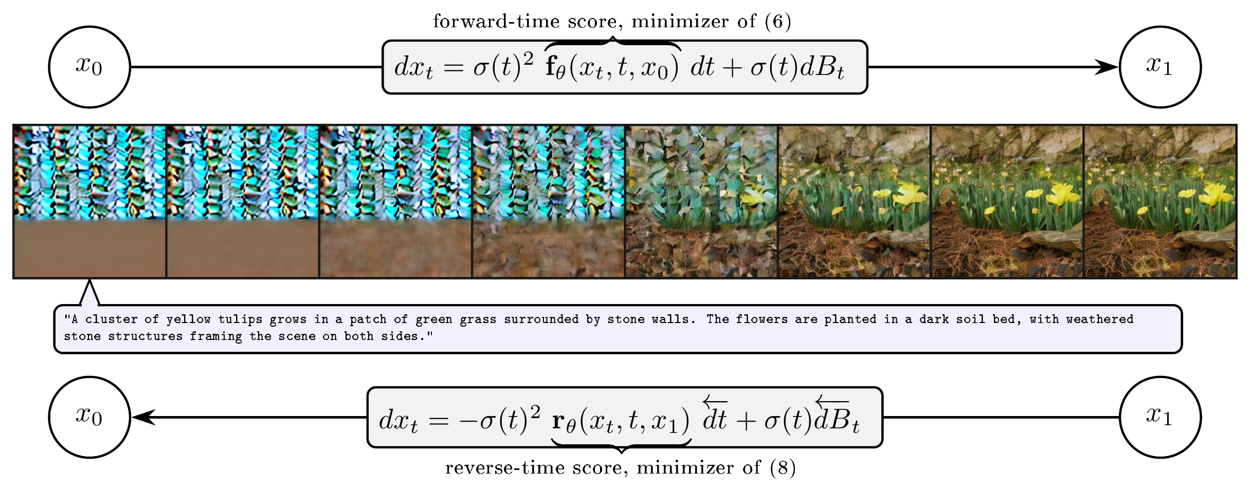
We want a stochastic process satisfying endpoint law $(X_0, X_1) \sim p_{{data}}$, where $X_0$ can be text and $X_1$ can be image representations. $p_{{data}}$ denotes the population joint law of the paired endpoints, and $p_{{data}}(X_0), p_{{data}}(X_1)$ denote its marginals. It should be simulatable in forward and reverse time.

Population and realizability convention. All objectives in this section are population objectives. Let $\mathbf f^\star$ and $\mathbf r^\star$ denote the fixed jointly Borel conditional-expectation (equivalently, $h$-transform) versions of the forward and reverse oracle drifts constructed in Appendix A.1–Appendix A.2. Realizability means that their weighted- $L^2$ equivalence classes have representatives in the corresponding parameterized drift classes. Every exact global population minimizer agrees with the relevant oracle under the weighted training-input law. Whenever a drift is used as an SDE coefficient in an exact path-law statement, however, we use the fixed oracle version: equality only on a training-null-set complement does not by itself imply that an arbitrary pointwise modification defines the same, or a unique, SDE law. In practice, the networks are trained as finite-sample approximations of these objectives; no exact path-law claim is made for a finite trained model.

3.1 Data-Generating Process as Mixture of Endpoint-Pinned Bridges

Base Process We start with the data-independent base process $\left(X_t\right)_{t \in [0, 1]}$ whose dynamics follow

$ dX_t = \sigma(t)dB_t,\tag{3} $

where $B_t$ is Brownian motion under $\mathbb{P}$ and is independent of $X_0$, $\sigma(t)$ is a deterministic positive scalar function satisfying Assumption 4, and $X_0 \sim p_{{data}}(X_0)$. Let $p_{{base}}$ denote the transition density under $\mathbb{P}$; under this base measure, it is not required that $X_1 \sim p_{{data}}(X_1)$.

Data-Generating Measure Using the regular conditional bridge kernels of Equation 3's base process, we define a path measure $\mathbb{Q}$ with the desired joint endpoint law.[^1] Conditional on both endpoints, the path measure (and volatility structure) is the same as that of the original scaled Brownian motion:

[^1]: Those unfamiliar with measure theory can imagine "lucky" Brownian motion that hits the desired data.

$ \begin{aligned} (X_0, X_1) &\sim_{\mathbb{Q}} p_{{data}} \quad\text{(a)} \ \mathbb{Q}(d\omega | X_0=x_0, X_1=x_1) &= \mathbb{P}(d\omega | X_0=x_0, X_1=x_1) \quad\text{(b)} \end{aligned}\tag{4} $

Here the conditional laws are regular conditional Gaussian-bridge kernels, and $\mathbb{Q}$ is their mixture over $p_{{data}}$. The $h$-transform used below gives absolute continuity with respect to the base law only after restriction to each $\mathcal F_T$, $T<1$. We do not assert absolute continuity on the pinned terminal sigma-field $\mathcal F_1$; the endpoint is instead obtained from the almost-sure continuous extension of the bridge path. We next derive tractable SDEs for the forward ($X_0 \rightarrow X_1$) and reverse ($X_1 \rightarrow X_0$) dynamics, allowing us to simulate data generation in both directions under $\mathbb{Q}$.

3.2 Forward-Time Model and Training Objective (Text-to-Image)

In the following theorems, $p_{{base}}(x_t | x_0, x_1)$ is a probability distribution of $X_t$ under $\mathbb{P}$: we show in Appendix A.1 that it is Gaussian with parameters that are primitives of $\sigma(t)$.

########## {caption="Theorem 1: Forward-Time SDE and Objective"}

Fix a regular conditional kernel $x_0\mapsto p_{{data}}(dx_1\mid x_0)$, and let $\mathbf f^\star(x, t;x_0)$ be the resulting fixed Borel $h$-transform version of

$ \mathbb{E}{\mathbb{Q}}!\left[\nabla_x\log p{base}(X_1\mid x) , \middle|, X_t=x, \ X_0=x_0\right], \qquad 0<t<1, $

where the conditional-expectation equality is understood under the bridge sampling law. There exists a canonical weak solution $(\overrightarrow X, B)$ on $[0, 1)$ such that $\overrightarrow X_0\sim p_{{data}}(X_0)$, $B$ is Brownian with respect to the solution filtration and independent of $\overrightarrow X_0$, and, on every $[0, T]$ with $T<1$,

$ d\overrightarrow{X}_t = \sigma(t)^2\mathbf{f}^\star(\overrightarrow{X}_t, t; \overrightarrow{X}_0)dt + \sigma(t)dB_t, \qquad 0\le t<1.\tag{5} $

The process has an almost-sure continuous extension $\overrightarrow X_1=\lim_{t\uparrow1}\overrightarrow X_t$, and the law of the extended path on $C([0, 1];\mathbb{R}^d)$ is $\mathbb{Q}$. Moreover, $\mathbf f^\star$ is the unrestricted weighted- $L^2$ minimizer of

$ \overrightarrow{\mathcal{L}}({\mathbf{f}}\theta) = \underset{\substack{t \sim \mathcal{U}((0, 1)) \ (x_0, x_1) \sim p{{data}} \ x_t \sim p_{{base}}(x_t | x_0, x_1)}}{\mathbb{E}}\left[w(t)\left| \mathbf{f}\theta(x_t, t; x_0) - \nabla{x_t}\text{log }p_\text{base}(x_1 | x_t) \right|^2_{2}\right].\tag{6} $

The weight function $w:(0, 1) \to (0, \infty)$ is chosen subject to Assumption 6. Under realizability, every exact parameterized minimizer agrees with $\mathbf f^\star$ under the weighted training-input law.

Proof: See Appendix A.1.

Thm. Theorem 1 gives us the mathematical machinery to simulate the forward data translation process, e.g., from text at $X_0$ to images at $X_1$, giving samples from a fixed version of $p_{{data}}(dx_1\mid x_0)$ at the population oracle for $p_{{data}}(X_0)$-almost every $x_0$. It does this via (1) a data-generating SDE Equation (5) on finite horizons, with its endpoint supplied by continuous extension, that we can discretize numerically; (2) a neural network loss function Equation (6) that allows us to estimate this SDE's drift from data. We parameterize $\mathbf{f}_\theta$ with a transformer ([15]); behavior at out-of-distribution source endpoints is extrapolative rather than part of the exact theorem.

If instead we remove conditioning on $\overrightarrow{X}0$, the population objective uses the loss integrand $w(t)\left| \mathbf{f}\theta(x_t, t; \varnothing) - \nabla_{x_t}\text{log }p_\text{base}(x_1 | x_t) \right|^2_{2}$. The canonical projected drift $\bar{\mathbf f}$ is state-only. Corollary 13 constructs at least one weak solution with this fixed drift and the same one-time marginals as $\mathbb{Q}$; it makes no uniqueness or Markov-property claim about the selected law or other weak solutions. This marginal equivalence provides aggregate target calibration only: it does not identify the transition kernel from a fixed intermediate state or guarantee conditional round-trip fidelity, which we evaluate empirically. This state-only version does not require endpoint conditioning and is useful for the sampling schemes in Section 6.2 and Section 6.3. See Appendix B for details.

3.3 Reverse-Time Model and Training Objective (Image-to-Text)

########## {caption="Theorem 2: Reverse-Time SDE and Objective"}

Fix a regular conditional kernel $x_1\mapsto p_{{data}}(dx_0\mid x_1)$, and let $\mathbf r^\star(x, t;x_1)$ be the resulting fixed Borel $h$-transform version of

$ \mathbb{E}{\mathbb{Q}}!\left[\nabla_x\log p{base}(x\mid X_0) , \middle|, X_t=x, \ X_1=x_1\right], \qquad 0<t<1. $

The conditional-expectation equality is understood under the bridge sampling law. There exists a canonical weak solution $(\overleftarrow X, B)$ on reverse time $u\in[0, 1)$ such that $\overleftarrow X_0\sim p_{{data}}(X_1)$, $B$ is Brownian w.r.t. the solution filtration and independent of $\overleftarrow X_0$, and, on every $[0, T]$ with $T<1$,

$ d\overleftarrow{X}_u = \sigma(1-u)^2\mathbf{r}^\star(\overleftarrow{X}_u, 1-u; \overleftarrow{X}_0)du + \sigma(1-u)dB_u, \qquad 0\le u<1.\tag{7} $

The process has an almost-sure continuous extension at $u=1$, and

$ \operatorname{Law}\bigl((\overleftarrow X_{1-t})_{0\le t\le1}\bigr)=\mathbb{Q}. $

Moreover, $\mathbf r^\star$ is the unrestricted weighted- $L^2$ minimizer of

$ \overleftarrow{\mathcal{L}}(\mathbf{r}\theta) = \underset{\substack{t \sim \mathcal{U}((0, 1)) \ (x_0, x_1) \sim p{{data}} \ x_t \sim p_{{base}}(x_t | x_0, x_1)}}{\mathbb{E}}\left[w(t)\left| \mathbf{r}\theta(x_t, t; x_1) - \nabla{x_t}\text{log }p_\text{base}(x_t | x_0) \right|^2_{2}\right]\tag{8} $

with the same weight function as in Theorem 1. Under realizability, every exact parameterized minimizer agrees with $\mathbf r^\star$ under the weighted training-input law.

Proof: See Appendix A.2. Effectively, this is just a time-index inversion of Theorem 1.

This is Thm. Theorem 1's dual. It lets us translate data in the opposite direction: from image at $\overrightarrow{X_1}=\overleftarrow{X_0}$ to text at $\overrightarrow{X_0}=\overleftarrow{X_1}$, giving samples from a fixed version of $p_{{data}}(dx_0\mid x_1)$ for $p_{{data}}(X_1)$-almost every $x_1$. Similarly, it provides an SDE we can simulate in reverse-time, and a training objective for the neural network that provides the data-translating drift; there is also a selected state-only reverse-time weak solution with matching marginals in App. Appendix B (Corollary 14). Inputs outside the population support are not covered by the exact conditional-law statement.

3.4 Classifier-Free Guidance

Classifier-free guidance improves sample quality in diffusion models ([16]). We use the following CFG-inspired extrapolation between the endpoint-conditioned and unconditioned bridge drifts from Theorem 1–Theorem 2 and Corollary 13–Corollary 14. Here $\omega\ge 0$ is the guidance strength:

$ \begin{aligned} \mathbf{f}\theta(x_t, t, x_0, \omega) &= (1+\omega)\mathbf{f}\theta(x_t, t; x_0) - \omega\mathbf{f}\theta(x_t, t; \emptyset) \ \mathbf{r}\theta(x_t, t, x_1, \omega) &= (1+\omega)\mathbf{r}\theta(x_t, t; x_1) - \omega\mathbf{r}\theta(x_t, t; \emptyset). \end{aligned} $

Unlike standard diffusion CFG, this bridge-drift extrapolation is used here as an empirical heuristic; we do not claim that it samples from an analytically identified guided distribution.

4. From Discrete to Continuous Token Embeddings

Section Summary: To bridge discrete text with a continuous mathematical framework, the authors convert tokens into continuous vectors that match the exact size of image latents while remaining nearly invertible back to the original tokens. They achieve this by embedding each token independently with a fixed lookup table from a strong pretrained model, then training a small decoder network that recovers the correct token over 99 percent of the time. The embeddings are sized so that 64 tokens of 64 dimensions each produce the same total dimensionality as the image codes, allowing the diffusion bridge to operate uniformly on both modalities.

Criterion: We have one snag in this otherwise elegant continuous-space mathematical framework: text is discrete. We circumvent this by embedding text tokens into continuous space. This continuous representation must (1) form a near-invertible mapping with discrete text, so we get distinguishable outputs; (2) have the same dimensionality as image data, as per our mathematical framework.

Framework: (1) Towards invertibility, we embed each token independently without attending to the other tokens in the sequence. If we naively used the hidden state of each token after attending to all the other tokens, there would be too many possibilities for which continuous embedding corresponds to which token, complicating the learning task. Embedding each token independently effectively creates a lookup table whose number of entries is the same as the tokenizer vocabulary size, greatly simplifying the problem. Then, we just need a backbone language model that is powerful enough to create a distinct representation for each token, which we confirm empirically. (2) Towards dimensionality matching, we fix the number of tokens (by truncation if the caption is too long, by padding if the caption is too short) per caption, and fix the embedding dimension of each token; such that the total size is the same as the number of components in the image latent code.

Instantiation: (1) For token-to-embedding, we use Qwen3-Embedding-8B ([17]) to generate the token-by-token embedding lookup table, because it (a) is very expressive (b) supports truncation of the embedding dimensions to our desired size, via Matryoshka representations ([18]). For embedding-to-token, we train a small MLP with cross-entropy loss to convert embeddings into tokens: this achieves

5. Comparison to Other Model Classes

Section Summary: Models that begin generation from a text or image representation rather than pure noise can retain more relevant information about the desired output, at least early in the process, which is especially useful in round-trip translation tasks. A supporting theorem establishes this local information advantage for data-to-data bridges over noise-based ones under stated conditions, with the benefit holding throughout the trajectory in simple Gaussian cases. In addition, stochastic differential equations are better suited than deterministic ordinary differential equations for capturing the many possible images that could match a given text prompt, because the added noise allows modeling of multi-peaked distributions.

Noise-to-Data: Intuitively, starting the image/text generative process from a text/image representation should be semantically richer and more informative than starting from Gaussian noise.

########## {caption="Theorem 3: Local mutual-information advantage of a data-to-data bridge"}

Let $T$ denote a text representation, let $Y$ denote its paired image representation, and let $N$ be noise independent of $(T, Y)$. Consider the text-to-image and noise-to-image bridges

$ \begin{aligned} X_t^{\mathrm{TI}} &= a_t T + b_t Y + \eta_t Z, \quad\text{(a)} \ X_t^{\mathrm{NI}} &= a_t N + b_t Y + \eta_t Z', \quad\text{(b)} \end{aligned}\tag{9} $

where $Z$ and $Z'$ are independent noise variables, independent of all endpoints. Suppose that $a_0=1$, $b_0=0$, and $\eta_0=0$; $0<I(T;Y)<\infty$; and the functions $f(t) \coloneqq I(X_t^{\mathrm{TI}};Y), g(t) \coloneqq I(X_t^{\mathrm{NI}};Y)$ are right-continuous at $t=0$. Then there exists $\tau>0$ such that, for every $t\in[0, \tau)$,

$ I(X_t^{\mathrm{TI}};Y)

I(X_t^{\mathrm{NI}};Y). $

Proof: See Appendix D for proof and statement of the opposite direction.

Thm. Theorem 3 concerns settings in which the evolving state itself must retain the source information, as in the round-trip procedures of Section 6.2 and Appendix R. It does not compare against a standard conditional T2I sampler that retains the text prompt as side information throughout the trajectory, and with retained side information the theorem gives no ordering. The state-only comparison is relevant to the evaluated round-trip setting, where a suitable auxiliary condition need not be supplied a priori (e.g., for an uncaptioned source image).

WLOG, Thm. Theorem 3 is presented for the text-to-image direction, but it also applies to image-to-text (with flipped time). App. Appendix E shows that for positively correlated jointly Gaussian scalar random variables and under BIT's choice of interpolation coefficients, strict dominance holds for every $t\in[0, 1)$, so $\tau=1$. For arbitrary joint distributions, how far $\tau$ extends is an empirical question; our experiments (Section 6.2) are consistent with the hypothesis that $\tau$ covers a large range for text-to-image.

ODE vs. SDE: ODEs linking text modalities directly to image modalities should fail at modeling multi-peaked distributions, since ODEs are deterministic. So, distribution-to-distribution flow matching (without hacks like endpoint noise injection ([19, 20])) is unsuitable for modeling the range of images that could correspond to a text prompt, and vice versa. In contrast, SDEs (due to noise injection) have hope for modeling multi-peaked distributions.

6. Experiments

Section Summary: The experiments evaluate a bridge-based generative model called BIT against two ablations on a dataset of roughly 100 million text-image pairs, using the same transformer architecture and training setup for all methods. One baseline starts from noise rather than real data and conditions on the other modality, while the second replaces the stochastic bridge with a deterministic flow-matching ODE. Results on text-to-image and image-to-text tasks show that BIT matches or exceeds the baselines on standard quality metrics and substantially outperforms the deterministic approach, which struggles to capture the inherent multimodality of cross-modal translation; additional tests demonstrate its use for producing varied yet semantically related outputs in either direction.

Comparisons In choosing baselines, we assess the impact of (1) data-to-data versus noise-to-data interpolation in the generative process (corresponding to diffusion ([1])); and (2) probabilistic versus deterministic modeling in the cross-modality bridge (corresponding to flow-matching ([2])). The first baseline is therefore an ablation that replaces one endpoint of the bridge with i.i.d. Gaussian noise and passes the cross-modality information through cross-attention conditioning. For text-to-image generation, for example, we start from noise and condition the score network on the text tokens, as in common text-to-image models ([3]). For fairness, we keep the SDE volatility schedule fixed. The second baseline is an ablation where, instead of a stochastic process, we construct a deterministic ODE by flow matching ([2]) between coupled text-image pairs.

Model Architecture We build upon [10]'s diffusion transformers. We use consistent settings across baselines, to isolate the effects of transport stochasticity and endpoint. See App. Appendix H.

Dataset We use approximately 100 million images from the GPIC text-to-image dataset ([21]), with images preprocessed into Stable Diffusion VAE latents ([3]) and text preprocessed into Qwen embeddings ([17]). See Appendix I.

Training and Inference Details See App. Appendix G for hyperparameters. See App. Appendix O for training, and App. Appendix P for inference pseudocode. Generally, we use the same hyperparameters across baselines, so that the performance difference can be attributed to the endpoint choice and stochasticity in transport.

6.1 Conditional Text-to-Image and Image-to-Text Generation

Goals We benchmark generation quality and prompt adherence in both T2I and I2T directions.

Results See Table 1. BIT performs favorably compared to other methods. See Appendix J.1 for metrics.

Effect of Data-to-Data: For text-to-image generation, BIT is very close to noise-to-data diffusion's performance on FID and CLIP. On image-to-text, BIT is by far the best on generative perplexity, and second-best on CLIP. The performance advantage of noise-to-data diffusion is small but statistically significant at a confidence level equal to 95%.

\begin{tabular}{lrrrr}
  \toprule
  Method & FID ($\downarrow$) & CLIP T2I ($\uparrow$) & Gen PPL ($\downarrow$) & CLIP I2T ($\uparrow$) \\
  \midrule
  \textbf{\texttt{BIT}} & 6.23 & \textit{\textbf{27.10}} & \textbf{123.4} & \textit{\textbf{26.99}} \\
  Diffusion (ablate data end) & \textbf{5.73} & \textbf{27.13} & 178.2 & 26.42 \\
  Flow (ablate stochasticity) & 279.13 & 20.13 & 169.2 & \textbf{27.25} \\
  \bottomrule
  \end{tabular}

This suggests that the Gaussian source used in diffusion models is not inherently special.

Effect of Stochasticity: Data-to-data flow matching fares the worst on every metric besides image-to-text CLIP, in line with our expectations: multimodality translation is inherently a stochastic task, so a deterministic ODE model is unsuitable. Without auxiliary randomness, a deterministic source-to-target flow cannot represent non-degenerate conditional distributions; this expressivity limitation helps explain the orders-of-magnitude worse text-to-image FID observed for the flow baseline.

We interpret this not as a SoTA competitor that BIT defeats, but as a measurement that isolates one design axis. FlowTok ([20]) and CrossFlow ([22]) report strong text-to-image results using data-to-data couplings, but they additionally learn variational encoders with auxiliary contrastive objectives. Because the variational encoder injects noise, these components restore stochasticity to an otherwise deterministic transport and address the conditional-diversity limitation of a bare deterministic map. BIT instead obtains stochasticity natively from the bridge SDE. Our controlled comparison of the ODE and SDE baselines shows that the bare deterministic transport is unsuitable in this multimodal setting. That being said, its good performance on image-to-text CLIP indicates that captioning (at least within the GPIC distribution) may be a fairly low entropy task given image conditioning. However, its generative perplexity is the worst, indicating it has not mastered the syntactic nuances of text.

6.2 Cross-Modal Round-Trip Stochastic Variation

Goals An important task in AI-aided art and design is to create variations of input data; e.g., Midjourney can generate image variations ([23]), while ChatGPT can paraphrase documents.

:::: cols="1"

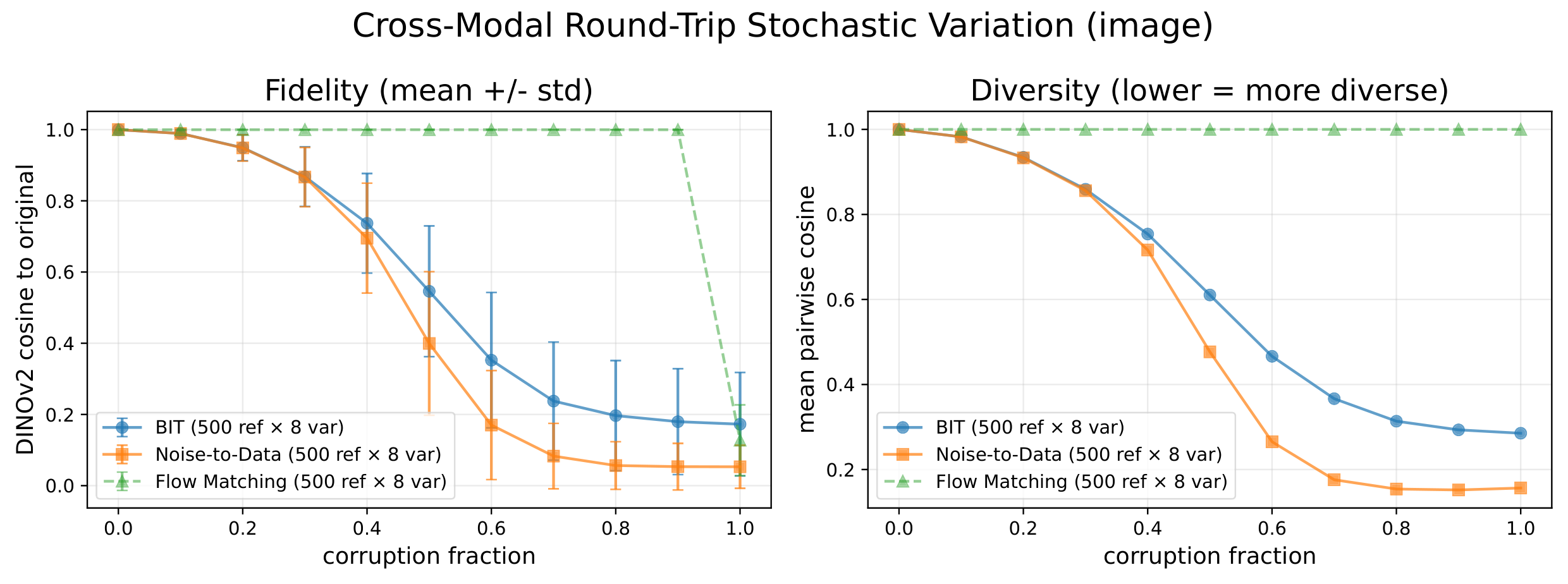
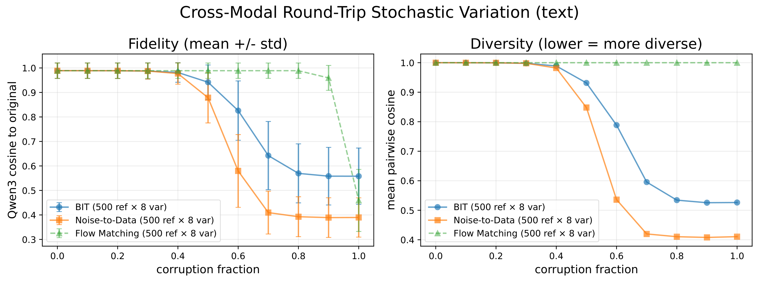
Figure 3: Cross-Modal Round-Trip Stochastic Variation: We want to generate semantically related variants of a given data sample. We run Algorithm 1 with $dt=0.004$ with Euler-Maruyama simulation. We compare BIT to denoising diffusion and data-to-data flow matching. App. Appendix T shows qualitative examples. ::::

With SDE-based (diffusion) generative models, a popular method to create data variations is to run a forward "noising" process, then restore the data through a time-reversed score-driven process, as popularized by SDEdit ([6]). The forward process removes fine details while retaining some high-level structure; time-reversed "denoising" then stochastically restores details consistent with that structure.

With noise-to-data diffusion models, increasing corruption progressively removes information about the original data. Thm. Theorem 3 motivates testing whether BIT retains useful source information for longer because its two data endpoints are dependent; the theorem itself is local near the source endpoint, so performance at high corruption levels is an empirical question.

Procedure We run Algorithm 1 on ground-truth samples at varying corruption levels. The marginal-equivalence corollaries motivate aggregate target calibration but don't guarantee source-conditioned reconstruction; semantic round-trip fidelity is evaluated empirically here. See Appendix J.2 for metrics.

Results See Figure 3, Figure 5, and Figure 6. Consistent with the information-retention motivation of Theorem 3, BIT's fidelity curve degrades more gracefully than that of the noise-to-data baseline at higher corruption fractions in both directions. Greater corruption also produces more diverse restorations. Noise-to-data diffusion exhibits greater diversity because its noise endpoint discards all source-state information, whereas BIT trades off fidelity and diversity.

6.3 Miscellaneous Comparisons

This subsection uses the billion-parameter model (trained on about 2x as many effective examples, with one network for both directions) from Appendix Q.

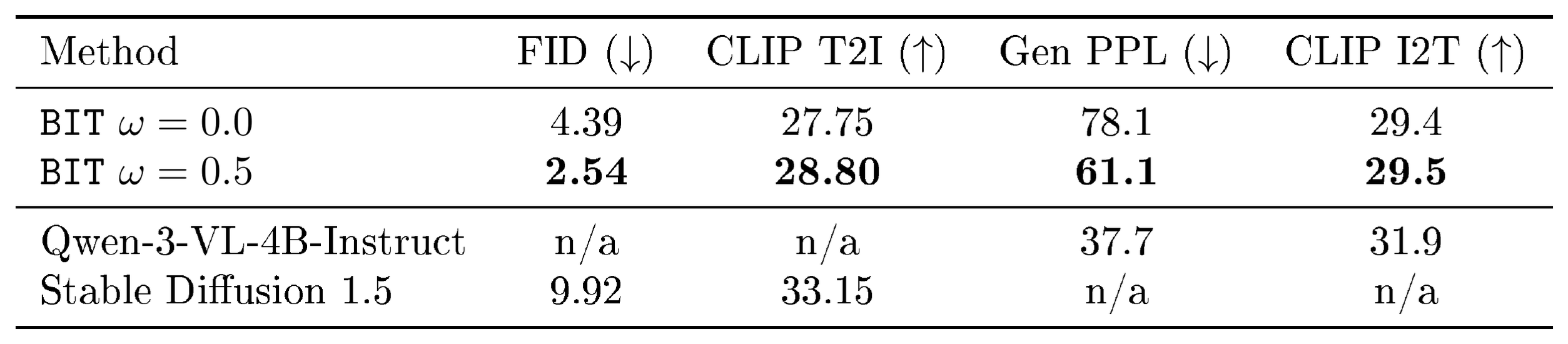
Impact of CFG: See Table 2. The CFG from Section 3.4 improves model performance for both text and image generation.

Impact of Scale and Engineering: Performance gains are possible with scale and engineering, as even $\omega=0$ in Table 2 exceeds all results in Table 1. This gives hope for industrial-scale BIT versions.

Anchors Against External Baselines: The previous subsections provide controlled scientific comparisons. Table 2 additionally reports external reference points, but these are not like-for-like comparisons: the models differ in training data, compute, architecture, and inference settings.

::: {caption="Table 2: Impact of CFG, and Comparison to Foundation Models. We use 500 SDE steps."}

:::

For I2T, BIT remains behind Qwen-3-VL-4B-Instruct ([7]), the model used to produce the GPIC reference captions, on both reported metrics. For T2I, BIT has a better FID than Stable Diffusion 1.5 ([3]) on the GPIC held-out distribution but a lower CLIP score.

6.4 Scientific Domain: Cell Fate Modeling

Goals Cell fate modeling studies how an early cellular state gives rise to later, differentiated outcomes. We evaluate BIT's ability to learn a conditional generative map between early progenitor cells and their later descendants in the $\textsc{Larry}$ lineage-tracing dataset ([24]). The model should generate realistic day-6 cell states from day-2 progenitors while preserving the fate and clone structure implied by lineage barcodes. So, a strong model must do more than match the marginal distribution of later cells: it must capture branching differentiation, place generated cells on the correct fate-specific trajectories, and support meaningful forward and reverse transport between progenitor and descendant states. See Appendix N for metrics.

Results Table 3 reports final test-set metrics. The cosine-volatility bridge has the best average rank (2.67), while different methods lead individual metrics. In particular, the cosine-volatility bridge obtains the highest fate kNN accuracy (0.445), and the separate-network uniform-volatility bridge has the best clone kNN and distributional MMD. These single-run ranks are descriptive; without uncertainty estimates, they do not establish statistical superiority. While endpoint regression obtains the lowest pointwise MSE, it substantially degrades distributional and biological structure, with the worst fate kNN accuracy and MMD among the methods. Rectified flow gives competitive MMD and cycle error, but has much worse forward and reverse MSE, indicating that its generated states match some marginal structure while failing to preserve the paired state-fate map.

\begin{tabular}{lcccccc c}
\toprule
Method & Fwd MSE $\downarrow$ & Rev MSE $\downarrow$ & Fwd MMD $\downarrow$
 {} & Fate kNN $\uparrow$ & Clone kNN $\uparrow$ & Cycle MSE $\downarrow$ & Avg. Rank $\downarrow$ \\
\midrule
\textbf{\texttt{BIT}, uniform shared} & 1.388 & 1.365 & 0.0446 & 0.404 & 0.182 & 1.307 / 1.418 & 3.33 \\
\textbf{\texttt{BIT}, uniform separate} & 1.415 & 1.394 & \textbf{0.0352} & 0.377 & \textbf{0.209} & 1.230 / 1.217 & 3.42 \\
\textbf{\texttt{BIT}, cosine shared} & 1.388 & 1.262 & 0.0431 & \textbf{0.445} & 0.160 & 1.042 / 1.136 & \textbf{2.67} \\
Noise-to-data diffusion & 1.329 & 1.381 & 0.0517 & 0.377 & 0.176 & 1.270 / 1.474 & 4.00 \\
Rectified flow & 2.444 & 1.694 & 0.0406 & 0.398 & 0.141 & \textbf{0.621 / 1.020} & 3.83 \\
Endpoint regression & \textbf{1.195} & \textbf{1.176} & 0.0847 & 0.336 & 0.047 & 1.076 / 1.102 & 3.75 \\
\bottomrule
\end{tabular}

6.5 Additional Results

See Appendix R for qualitative image-editing results, Appendix S for ablation on REPA.

7. Related Works, Discussion, Conclusion

Section Summary: This work builds on prior advances in diffusion bridges, data-to-data translation, and continuous-time language models while introducing BIT, a bidirectional image-text diffusion bridge that starts from text representations and interpolates toward images rather than following the usual noise-to-data path. Experiments show this approach matches or outperforms traditional baselines on several tasks and enables flexible generation and round-trip sampling in both directions within a single framework. The authors also outline plans for future multi-domain extensions and studies of how endpoint geometry influences performance.

Our work builds on advances in diffusion bridges ([10, 11, 25]), data-to-data translation models ([26, 22]), and continuous-time and space language generation ([5, 26, 27]). See Appendix U for more related work. In future work, we hope to explore translation across many domains, e.g., text-image-audio. We also want to conduct a systematic study of how endpoint geometry affects bridge performance. In this work, we introduced BIT: Bidirectional Image-Text Diffusion Bridges. BIT challenges the traditional noise-to-data paradigm for T2I generation: in our controlled experiments, starting from a text representation and interpolating toward images is competitive with the noise-to-data baseline and performs better on several downstream tasks. The endpoint-conditioned construction supports generation in both directions, while its source-aware path enables flexible round-trip sampling within a unified T2I and I2T framework.

AI use statement

In this work, we used generative AI tools for helping to: write mathematical proofs, write code, and draft some descriptions of experimental details. We have manually reviewed all AI-assisted work (proofs, code, writing), and affirm to the best of our knowledge that it is correct.

Acknowledgments

This material is based upon work supported by the U.S. Department of Energy, Office of Science, Office of Advanced Scientific Computing Research, Department of Energy Computational Science Graduate Fellowship under Award Number DE-SC0025528. This research used resources of the National Energy Research Scientific Computing Center (NERSC), a Department of Energy User Facility (projects m5319-2026, m1266-2026). J. Blanchet gratefully acknowledges support from ONR under award N00014-24-1-2655, and the National Science Foundation (NSF) under grants 2312204 and 2403007.

We thank Yangyi Shen, Lutong Hao, and Miguel Liu-Schiaffini for helpful discussion.

Appendix

Section Summary: This appendix derives the core theoretical machinery for constructing a stochastic bridge process whose endpoints follow a joint data distribution Π. Starting from a conditionally Gaussian process, it defines an SDE whose drift incorporates a time-dependent tilted mean that anticipates the unknown endpoint, ensuring the path measure matches the desired conditional law. Under standard regularity conditions on volatility and moments, the construction yields a weak solution that extends continuously to the terminal time with the correct marginal distribution.

A. Conditional Stochastic Process Derivation

This section provides a self-contained derivation of the theoretical results underlying our algorithmic approach, prioritizing clarity and accessibility over maximum generality. Throughout this section, we denote the population data-generating law as $\Pi \in \Delta((\mathbb{R}^d)^2)$.

Under the base measure $\mathbb{P}$, the process $X_{\cdot}$ defined in Equation 3 is conditionally Gaussian: $(X_t){t \in [0, 1]} \vert X_0$ is a Gaussian process. Therefore, conditional on both endpoints, $(X_t){t \in [0, 1]} \vert X_0, X_1$ is also a Gaussian process.

This conditional Gaussian process is a bridge pinned at both endpoints. We denote the law of the Gaussian bridge with endpoints $(x_0, x_1) \in (\mathbb{R}^d)^2$ by $\mathbb{P}^{(x_0, x_1)}$. Therefore,

$ \mathbb{Q}(A) = \int_{(x_0, x_1) \in (\mathbb{R}^d)^2} \mathbb{P}^{(x_0, x_1)}(A) \Pi(dx_0, dx_1)\tag{10} $

for any measurable set $A$. Write $\Pi_0$ and $\Pi_1$ for the first and second marginals of $\Pi$.

########## {caption="Assumption 4"}

Assume that $0 < \underline{\sigma} \le \sigma(t) \le \bar{\sigma}$ for all $t \in [0, 1]$, that $\sigma$ is continuous, and that the endpoint coupling has finite second moments:

$ \mathbb{E}_{\Pi}!\left[\lVert X_0\rVert_2^2+\lVert X_1\rVert_2^2\right]<\infty. $

Under this assumption, $\sigma$ is square-integrable. Moreover, we define

$ a(t) := \int_{s=0}^t \sigma(s)^2 ds, $

so $a:[0, 1] \to [0, \infty)$ is increasing and Lipschitz continuous. Because $\sigma^2$ is continuous, the fundamental theorem of calculus also gives $a\in C^1([0, 1])$ with $a'(t)=\sigma(t)^2$.

Gaussian/Brownian Bridge Construction

Regarding the proofs to follow, it is useful to anchor them in the context of the well-known Brownian bridge machinery ([28]).

It is known that ([13]), by defining $(X^{(x_0, x_1)}t){t\in [0, 1)}$ via the SDE

$ \begin{aligned} \begin{cases} X^{(x_0, x_1)}_0 &= x_0\ dX^{(x_0, x_1)}_t &= \frac{\sigma(t)^2}{a(1)-a(t)}[x_1 - X^{(x_0, x_1)}_t] dt + \sigma(t) dB_t \end{cases}, \end{aligned} $

we will have that a strong solution exists on $[0, 1)$ with a unique continuous extension throughout $[0, 1]$; such solution has law $\mathbb{P}^{(x_0, x_1)}$.

Now fix only the initial endpoint $x_0$ and let $X_1$ have a distribution $F_1 \in \Delta(\mathbb{R}^d)$ with finite second moments. On the half-open interval $[0, 1)$, consider the SDE

$ \begin{aligned} \begin{cases} X^{(x_0, F_1)}_0 &= x_0\ dX^{(x_0, F_1)}_t &= \frac{\sigma(t)^2}{a(1)-a(t)} [m(t, X^{(x_0, F_1)}_t; x_0, F_1) - X^{(x_0, F_1)}_t] dt + \sigma(t) dB_t \end{cases}, \end{aligned}\tag{11} $

where the equation is understood on every finite horizon $[0, T]$, $T<1$ (the value of the drift at the single time $t=0$ may be chosen arbitrarily), and where, for $0<t<1$, the tilted mean function is

$ m(t, x_t; x_0, F_1) := \frac{\int_{y \in \mathbb{R}^d} y e^{-\frac{\left\Vert (y-x_0) - (x_t-x_0)\frac{a(1)}{a(t)}\right\Vert_2^2}{2 \frac{a(1)(a(1)-a(t))}{a(t)}}} F_1(dy)}{\int_{y \in \mathbb{R}^d} e^{-\frac{\left\Vert (y-x_0) - (x_t-x_0)\frac{a(1)}{a(t)}\right\Vert_2^2}{2 \frac{a(1)(a(1)-a(t))}{a(t)}}} F_1(dy)}. $

The mixture measure

$ \mathbb{P}^{(x_0, F_1)} :=\int_{\mathbb{R}^d}\mathbb{P}^{(x_0, y)}F_1(dy) $

will provide a canonical weak solution law of this SDE. Its endpoint is supplied by the continuous extension, not by evaluating the singular drift at $t=1$.

A heuristic way to motivate the correctness of this is that the tilted mean (which was written as a weighted average over Gaussian PDFs) is indeed

$ \begin{aligned} m(t, x_t; x_0, F_1) &= \mathbb{E}{(X_r){r\in [0, 1]} \sim \mathbb{P}^{(x_0, F_1)}}\left[X_1 \vert X_t = x_t\right]\ &= \mathbb{E}{(X_r){r\in [0, 1]} \sim \mathbb{P}^{(x_0, F_1)}}\left[X_1 \vert X_t = x_t, (X_s)_{s=0}^t\right], \end{aligned} $

so $m(t, X^{(x_0, F_1)}_t;x_0, F_1)$ is the mean of the endpoint $X^{(x_0, F_1)}_1$ given the Brownian filtration at the current time $\mathcal{F}_t$. To see why, we note (and will later show rigorously) that $X^{(x_0, x_1)}_t$ is distributed according to the pdf

$ \begin{aligned} p(x_t; x_0, x_1) &= \left(2\pi \frac{a(t)(a(1)-a(t))}{a(1)}\right)^{-\frac{d}{2}} e^{-\frac{\left\Vert (x_t-x_0) - (x_1-x_0)\frac{a(t)}{a(1)}\right\Vert_2^2}{2 \frac{a(t)(a(1)-a(t))}{a(1)}}}\ &= \left(2\pi \frac{a(t)(a(1)-a(t))}{a(1)}\right)^{-\frac{d}{2}} e^{-\frac{\left\Vert (x_1-x_0) - (x_t-x_0)\frac{a(1)}{a(t)}\right\Vert_2^2}{2 \frac{a(1)(a(1)-a(t))}{a(t)}}}. \end{aligned} $

########## {caption="Lemma 5"}

For any $x_0\in\mathbb{R}^d$, under $\mathbb{P}^{(x_0, F_1)}$ the coordinate process is a weak solution of Equation 11 on every $[0, T]$, $T<1$. It has an almost-sure continuous extension to $t=1$, with $X_1\sim F_1$. Thus $\mathbb{P}^{(x_0, F_1)}$ is the canonical weak solution law associated with Equation 11; no uniqueness assertion is made for arbitrary pointwise versions of its drift.

Intuitively, we have Lemma 5 to rigorously show that the SDE described in Equation 11 does indeed have the correct data-generating path measure.

Proof: Denote $\mathbb{P}^{(x_0)}$ as a path measure of $X_t := x_0 + \int_{0}^{t}\sigma(s)dB_s$, so

$ \mathbb{P}^{(x_0, x_1)}(\cdot) = \mathbb{P}^{(x_0)}(\cdot \vert X_1=x_1). $

The distribution of $X_t$ under $\mathbb{P}^{(x_0)}$ is $N(x_0, a(t)I)$ for any $t \in [0, 1]$, and the distribution of $X_t \vert X_s$ where $0 \le s\le t \le 1$ is $N(X_s, (a(t)-a(s))I)$.

This means that, with $\lambda$ being the Lebesgue measure, for any $t \in [0, 1)$,

$ \begin{aligned} \frac{d\mathbb{P}^{(x_0)}(X_1=\cdot \vert X_t)}{d\mathbb{P}^{(x_0)}(X_1=\cdot)} (x_1) &= \frac{ \frac{d\mathbb{P}^{(x_0)}(X_1=\cdot \vert X_t)}{d\lambda(\cdot)} (x_1) } { \frac{d\mathbb{P}^{(x_0)}(X_1=\cdot)}{d\lambda(\cdot)} (x_1) }\ &= \frac{ (2\pi (a(1)-a(t)))^{-\frac{d}{2}} e^{- \frac{\Vert x_1 - X_t\Vert_2^2}{2(a(1)-a(t))}} } { (2\pi a(1))^{-\frac{d}{2}} e^{- \frac{\Vert x_1 - x_0\Vert_2^2}{2a(1)}} }\ &= \left(\frac{a(1)}{a(1)-a(t)}\right)^{\frac{d}{2}} e^{\frac{\Vert x_1 - x_0\Vert_2^2}{2a(1)}- \frac{\Vert x_1 - X_t\Vert_2^2}{2(a(1)-a(t))}} \end{aligned}\tag{12} $

almost everywhere $x_1$ and almost surely $X_t$.

Thus, we define, for any $x_1\in \mathbb{R}^d$, a random process

$ Z^{(x_0, x_1)}_t := \left(\frac{a(1)}{a(1)-a(t)}\right)^{\frac{d}{2}} e^{\frac{\Vert x_1 - x_0\Vert_2^2}{2a(1)}- \frac{\Vert x_1 - X_t\Vert_2^2}{2(a(1)-a(t))}}.\tag{13} $

Crucially, Equation 13 has the same expression as Equation 12. We defined Equation 13 because Equation 12 is technically not defined everywhere (although its undefined set has measure zero), which makes operations such as integration ill-defined without choosing a version. In contrast, Equation 13 is defined everywhere and provides a convenient version of this fixed-time Bayes density.

Now, we want to show that this random process (which corresponds to the change-of-measure) is a martingale. For $0 \le s<t < 1$, we have that

$ \begin{aligned} \mathbb{E}^{\mathbb{P}^{(x_0)}}\left[Z^{(x_0, x_1)}_t \middle\vert \mathcal{F}_s \right] &= \frac{ \mathbb{E}^{\mathbb{P}^{(x_0)}}\left[(2\pi (a(1)-a(t)))^{-\frac{d}{2}} e^{- \frac{\Vert x_1 - X_t\Vert_2^2}{2(a(1)-a(t))}} \middle\vert \mathcal{F}s \right] } { (2\pi a(1))^{-\frac{d}{2}} e^{- \frac{\Vert x_1 - x_0\Vert_2^2}{2a(1)}} }\ &= \frac{ \mathbb{E}{Z \sim N(0, I)}\left[(2\pi (a(1)-a(t)))^{-\frac{d}{2}} e^{- \frac{\Vert x_1 - X_s+\sqrt{a(t)-a(s)}Z\Vert_2^2}{2(a(1)-a(t))}} \middle\vert X_s \right] } { (2\pi a(1))^{-\frac{d}{2}} e^{- \frac{\Vert x_1 - x_0\Vert_2^2}{2a(1)}} }\ &= \frac{ (2\pi (a(1)-a(s)))^{-\frac{d}{2}} e^{- \frac{\Vert x_1 - X_s\Vert_2^2}{2(a(1)-a(s))}} } { (2\pi a(1))^{-\frac{d}{2}} e^{- \frac{\Vert x_1 - x_0\Vert_2^2}{2a(1)}} }\ &= Z^{(x_0, x_1)}_s. \end{aligned} $

The cancellation of the auxiliary random variable $Z$ follows from the convolution of two Gaussian densities.

The displayed conditional-expectation identity proves that $\left(Z^{(x_0, x_1)}t\right){t \in [0, 1)}$ is a martingale with respect to $\mathbb{P}^{(x_0)}$; its positivity ensures integrability once $\mathbb{E}[Z_t]=Z_0=1$ is established.

We now work from the already defined bridge mixture rather than trying to extend a finite-horizon density to the pinned terminal sigma-field. Define the harmonic function ([13]), for all $t\in(0, 1)$ and $x\in\mathbb{R}^d$, by

$ h(t, x) := \int_{y \in \mathbb{R}^d} \left(\frac{a(1)}{a(1)-a(t)}\right)^{\frac{d}{2}} e^{\frac{\Vert y - x_0\Vert_2^2}{2a(1)}- \frac{\Vert y - x\Vert_2^2}{2(a(1)-a(t))}} F_1(dy). $

This is the $F_1$-mixture of the martingales $Z_t^{(x_0, y)}$. For each compact subinterval of $(0, 1)$, the negative quadratic term provides an integrable bound for the kernel and its required derivatives. Hence Tonelli's theorem and differentiation under the integral give $h>0$, $h\in C^{1, 2}$, and the backward harmonic equation.

Fix $T<1$. By the finite-horizon Bayes identity above, for every bounded $\mathcal F_T$-measurable random variable $G$,

$ \begin{aligned} \mathbb{E}^{\mathbb{P}^{(x_0, F_1)}}[G] &=\int_{\mathbb{R}^d}\mathbb{E}^{\mathbb{P}^{(x_0, y)}}[G] F_1(dy)\ &=\mathbb{E}^{\mathbb{P}^{(x_0)}}!\left[G\int_{\mathbb{R}^d}Z_T^{(x_0, y)}F_1(dy)\right]\ &=\mathbb{E}^{\mathbb{P}^{(x_0)}}[G h(T, X_T)]. \end{aligned} $

Consequently,

$ \left.\frac{d\mathbb{P}^{(x_0, F_1)}}{d\mathbb{P}^{(x_0)}} \right|_{\mathcal F_T}=h(T, X_T), $

a statement made only for $T<1$. In particular, this calculation neither asserts nor requires absolute continuity on $\mathcal F_1$; for singular $F_1$ such terminal absolute continuity is false, and the density martingale need not be uniformly integrable.

The finite-horizon $h$-transform/Girsanov theorem ([12]) now shows that, for every $T<1$,

$ B_t^{(x_0, F_1)} :=B_t-\int_0^t\sigma(s)\nabla_x\log h(s, X_s), ds, \qquad 0\le t\le T, $

is Brownian under $\mathbb{P}^{(x_0, F_1)}$. These definitions are consistent as $T$ varies and therefore define one Brownian motion on $[0, 1)$.

Direct differentiation of $h$ yields $\nabla_x\log h(t, x)=[m(t, x;x_0, F_1)-x]/[a(1)-a(t)]$. Thus, on every finite horizon,

$ \begin{aligned} dX_t &=\frac{\sigma(t)^2}{a(1)-a(t)} [m(t, X_t;x_0, F_1)-X_t] dt +\sigma(t)dB_t^{(x_0, F_1)}. \end{aligned} $

Finally, the continuous extension and its terminal law $F_1$ hold by the definition of $\mathbb{P}^{(x_0, F_1)}$ as a mixture of continuously extended pinned bridge laws. This proves the claimed canonical weak-solution result.

Next, we will prove the main theorem (Theorem 1).

A.1 Proof of Forward Process SDE and Objective

Before proving the theorem, we first provide the regularity assumption we impose on the weight function $w: (0, 1) \to (0, \infty)$.

########## {caption="Assumption 6"}

There exist constants $C_0, C_1, \beta_0, \beta_1>0$ such that

$ w(t) \le \min!\left(C_0t^{\beta_0}, C_1(1-t)^{\beta_1}\right), $

and $w(\cdot)$ is continuous.

This assumption controls the contribution of the sample close to the two endpoints. Moreover, this can also be incorporated as importance sampling as well as other variance reduction methods.

Under this assumption, we can prove the following lemma.

########## {caption="Lemma 7"}

Under the Assumption 4, Assumption 6, we have that

$ \int_{t=0}^1 \frac{1}{a(t)(a(1)-a(t))} w(t)dt < \infty. $

Proof: Fix any $\epsilon\in(0, \tfrac12)$. From continuity, the integrand is bounded on $[\epsilon, 1-\epsilon]$, so it suffices to show that

$ \int_{t=0}^{\epsilon}\frac{w(t), dt}{a(t)\bigl(a(1)-a(t)\bigr)} +\int_{t=1-\epsilon}^{1}\frac{w(t), dt}{a(t)\bigl(a(1)-a(t)\bigr)}<\infty . $

Since $\sigma(t)\in[\underline{\sigma}, \overline{\sigma}]\subseteq(0, \infty)$, integrating the lower bound gives

$ a(t)=\int_{0}^{t}\sigma(s)^{2}, ds;\ge;\underline{\sigma}^{2}t, \qquad a(1)-a(t)=\int_{t}^{1}\sigma(s)^{2}, ds;\ge;\underline{\sigma}^{2}(1-t). $

For $t\le\epsilon$ we have $1-t\ge 1-\epsilon$, hence $a(1)-a(t)\ge\underline{\sigma}^{2}(1-\epsilon)$, and we further have that the first term satisfies

$ \begin{aligned} \int_{t=0}^{\epsilon}\frac{w(t), dt}{a(t)\bigl(a(1)-a(t)\bigr)} &\le\frac{1}{\underline{\sigma}^{4}(1-\epsilon)}\int_{t=0}^{\epsilon}\frac{w(t)}{t}, dt\ &\le\frac{C_0}{\underline{\sigma}^{4}(1-\epsilon)}\int_{t=0}^{\epsilon}t^{, \beta_0-1}, dt\ &=\frac{C_0}{\underline{\sigma}^{4}(1-\epsilon)}\cdot\frac{\epsilon^{, \beta_0}}{\beta_0}<\infty, \end{aligned} $

where we used $w(t)\le C_0t^{\beta_0}$ from Assumption 6 and $\beta_0>0$.

The same argument goes for the second integral, with the roles of the two endpoints exchanged: for $t\ge 1-\epsilon$ we have $a(t)\ge\underline{\sigma}^{2}(1-\epsilon)$ and $a(1)-a(t)\ge\underline{\sigma}^{2}(1-t)$, so with $w(t)\le C_1(1-t)^{\beta_1}$,

$ \int_{t=1-\epsilon}^{1}\frac{w(t), dt}{a(t)\bigl(a(1)-a(t)\bigr)} \le\frac{C_1}{\underline{\sigma}^{4}(1-\epsilon)}\int_{t=1-\epsilon}^{1}(1-t)^{, \beta_1-1}, dt =\frac{C_1}{\underline{\sigma}^{4}(1-\epsilon)}\cdot\frac{\epsilon^{, \beta_1}}{\beta_1}<\infty. \blacksquare $

########## {caption="Lemma 8: Weighted square-integrability of the score targets"}

Under Assumption 4 and Assumption 6, both score targets in Equations 6 and 8 belong to their weighted $L^2$ spaces.

Proof: Write $A=a(1)$ and $\Delta=X_1-X_0$. The bridge sampling formula

$ X_t=\left(1-\frac{a(t)}A\right)X_0+\frac{a(t)}A X_1 +\sqrt{\frac{a(t)(A-a(t))}{A}}, Z,\tag{14} $

holds with $Z\sim N(0, I_d)$ independent of $(X_0, X_1)$. Consequently,

$ \begin{aligned} \Phi_f &:=\nabla_{X_t}\log p_{base}(X_1\mid X_t) =\frac{\Delta}{A} -\sqrt{\frac{a(t)}{A(A-a(t))}}, Z, \ \Phi_r &:=\nabla_{X_t}\log p_{base}(X_t\mid X_0) =-\frac{\Delta}{A} -\sqrt{\frac{A-a(t)}{Aa(t)}}, Z. \end{aligned} $

Independence and centering of $Z$ give

$ \begin{aligned} \mathbb{E}|\Phi_f|_2^2 &=\frac{\mathbb{E}|\Delta|_2^2}{A^2} +\frac{d, a(t)}{A(A-a(t))}, \ \mathbb{E}|\Phi_r|_2^2 &=\frac{\mathbb{E}|\Delta|_2^2}{A^2} +\frac{d(A-a(t))}{Aa(t)}. \end{aligned} $

The endpoint term is finite by Assumption 4. Moreover,

$ \frac{a(t)}{A-a(t)}\le \frac{A^2}{a(t)(A-a(t))}, \qquad \frac{A-a(t)}{a(t)}\le \frac{A^2}{a(t)(A-a(t))}, $

and $\int_0^1w(t), dt<\infty$. Lemma 7 therefore makes the weighted time integrals of both displayed second moments finite.

Proof of Theorem 1 (score-matching objective).

Proof: Let $\Pi_0$ be the first marginal of $\Pi$ and fix a regular conditional kernel $x_0\mapsto\Pi_1^{x_0}$ for $X_1$ given $X_0=x_0$. The spaces are standard Borel, so such a kernel and the jointly Borel versions below exist. Under the sampling law in Equation 6, set

$ \mathbf f^\star(X_t, t;X_0) :=\mathbb{E}[\Phi_f\mid X_t, t, X_0], $

choosing the $h$-transform version

$ \mathbf f^\star(x, t;x_0) =\frac{m(t, x;x_0, \Pi_1^{x_0})-x}{a(1)-a(t)}\tag{15} $

for $0<t<1$ and $\Pi_0$-almost every $x_0$. Lemma 8 justifies the $L^2$ conditional expectation. The Pythagorean identity gives, for every square-integrable candidate $f$,

$ \overrightarrow{\mathcal L}(f) =\overrightarrow{\mathcal L}(\mathbf f^\star) +\mathbb{E}!\left[w(t)|f(X_t, t;X_0) -\mathbf f^\star(X_t, t;X_0)|_2^2\right]. $

Thus $\mathbf f^\star$ is the unrestricted minimizer, and realizability implies that every exact parameterized minimizer agrees with it under the weighted training-input law. This conclusion concerns an $L^2$ equivalence class; the SDE below uses the fixed version equation 15.

For $\Pi_0$-almost every $x_0$, Lemma 5 applied with $F_1=\Pi_1^{x_0}$ makes the coordinate process under $\mathbb{P}^{(x_0, \Pi_1^{x_0})}$ a weak solution of Equation 5 on every $[0, T]$, $T<1$. Mixing these laws over $\Pi_0(dx_0)$ gives

$ \int\mathbb{P}^{(x_0, \Pi_1^{x_0})}\Pi_0(dx_0) =\int\mathbb{P}^{(x_0, x_1)}\Pi(dx_0, dx_1)=\mathbb{Q}. $

Conditionally on each initial value, the innovation in the finite-horizon $h$-transform is a standard Brownian motion with the same Wiener law. Hence, after mixing, it is independent of $\overrightarrow X_0$. Finally, continuous extension at $t=1$ follows from the mixture-of-pinned-bridges construction, and the extended path law is $\mathbb{Q}$.

########## {caption="Remark"}

The theorem is a population-level oracle statement under realizability. Practical training may incur estimation, optimization, and approximation error. Even at the population optimum, an arbitrary modification of a minimizer on a training-null set is not automatically an interchangeable SDE coefficient; the exact path-law conclusion uses the canonical version displayed above.

A.2 Proof of Reverse Process SDE and Objective

The proof for this theorem (Theorem 2) mirrors the proof of Theorem 1 but with the flipped time notations (and appropriately mirrored coefficients).

Proof of Theorem 2: Consider the endpoint-swapped coupling

$ (X'_0, X'_1) \coloneqq (X_1, X_0) $

and define the reversed volatility schedule and weight by

$ \sigma'(u) \coloneqq \sigma(1-u), \qquad w'(u) \coloneqq w(1-u). $

The corresponding integrated variance is

$ \begin{aligned} a'(u) &\coloneqq \int_0^u \sigma'(s)^2, ds \ &= \int_0^u \sigma(1-s)^2, ds \ &= a(1)-a(1-u). \end{aligned} $

In particular,

$ a'(1)-a'(u)=a(1-u). $

Applying Theorem 1 to the swapped coupling and the volatility schedule $\sigma'$ gives a forward process $(\overleftarrow{X}u){u\in[0, 1)}$ starting from

$ \overleftarrow{X}0\sim p{\mathrm{data}}(X_1). $

Its canonical population drift is the fixed Borel version

$ \begin{aligned} \mathbf r^\star(x, 1-u;x_1) &= \mathbb{E} \left[\nabla_x \log p_{\mathrm{base}}(x\mid X_0) , \middle|, X_1=x_1, \ X_{1-u}=x \right] \ &= \frac{ \mathbb{E}[X_0\mid X_1=x_1, \ X_{1-u}=x]-x }{ a(1-u) }. \end{aligned} $

Therefore, the resulting SDE is

$ d\overleftarrow{X}_u

\sigma(1-u)^2 \mathbf r^\star(\overleftarrow{X}_u, 1-u; \overleftarrow{X}_0), du + \sigma(1-u), dB_u, $

which is exactly Equation 7.

Lemma 8 first establishes that the target in Equation 8 belongs to the relevant weighted $L^2$ space. Changing variables according to $t=1-u$ transforms the forward objective for the swapped process into Equation 8, and $w'$ satisfies Assumption 6, with the constants and endpoint exponents interchanged. The same Pythagorean identity used in the forward proof therefore shows that $\mathbf r^\star$ is the unrestricted minimizer and that every exact realizable parameterized minimizer agrees with it under the weighted training-input law. The reverse SDE nevertheless uses the fixed displayed version, not an arbitrary representative of that class.

For completeness, the reversal of the bridge law follows directly from its Gaussian mean and two-time covariance. For $s\le t$, the conditional covariance of the original bridge is

$ \operatorname{Cov}(X_s, X_t\mid X_0, X_1) =\frac{a(s)(a(1)-a(t))}{a(1)}I_d. $

Together with $a'(u)=a(1)-a(1-u)$, this shows that the $\sigma'$-bridge from $(x_1, x_0)$ is exactly the image of the $\sigma$-bridge from $(x_0, x_1)$ under $\omega(t)\mapsto\omega(1-t)$. Theorem 1 applied to the swapped coupling thus gives, after the almost-sure continuous extension at $u=1$,

$ \operatorname{Law} \bigl((\overleftarrow{X}{1-t}){t\in[0, 1]} \bigr)

\mathbb{Q}, $

as claimed. Its innovation Brownian motion is independent of the reverse initial endpoint by the independence statement in the forward construction.

Alternatively, we could prove this via Anderson's time-reversal ([29]).

B. Marginal SDEs

########## {caption="Lemma 9: Endpoint projection"}

Let $\Pi$ be the endpoint law and let

$ K_t((x_0, x_1), dx) :=p_{base}(x\mid x_0, x_1), dx, \qquad 0<t<1, $

be the Gaussian bridge kernel. With $Z_w:=\int_0^1w(t), dt$, define the probability measure

$ \nu(dt, dx_0, dx_1, dx) :=Z_w^{-1}w(t), dt, \Pi(dx_0, dx_1) K_t((x_0, x_1), dx).\tag{16} $

Suppose that the Borel target $\Phi(x, t, x_0, x_1)$ belongs to $L^2(\nu)$. Let $\kappa_{t, x}(dx_0, dx_1)$ be a regular conditional endpoint kernel under $\nu$ given $(t, X_t)=(t, x)$; let $\kappa^0_{t, x}$ and $\kappa^1_{t, x}$ be its marginals, and fix conditional kernels $\kappa^{1\mid0}{t, x, x_0}(dx_1)$ and $\kappa^{0\mid1}{t, x, x_1}(dx_0)$. Then jointly Borel versions of the three unrestricted square-loss minimizers are

$ \begin{aligned} \phi_\varnothing^\star(x, t) &=\int\Phi(x, t, x_0, x_1), \kappa_{t, x}(dx_0, dx_1), \ \phi_0^\star(x, t;x_0) &=\int\Phi(x, t, x_0, x_1), \kappa^{1\mid0}{t, x, x_0}(dx_1), \ \phi_1^\star(x, t;x_1) &=\int\Phi(x, t, x_0, x_1), \kappa^{0\mid1}{t, x, x_1}(dx_0). \end{aligned} $

They satisfy, for the $(t, X_t)$-marginal of $\nu$-almost every $(t, x)$,

$ \phi_\varnothing^\star(x, t) =\int\phi_0^\star(x, t;x_0), \kappa^0_{t, x}(dx_0) =\int\phi_1^\star(x, t;x_1), \kappa^1_{t, x}(dx_1).\tag{17} $

Under realizability, every exact parameterized population minimizer agrees with its corresponding displayed oracle under the relevant marginal of $\nu$. The displayed Borel versions, rather than arbitrary modifications on $\nu$-null sets, are used below as SDE coefficients.

Proof: All state spaces are standard Borel, so the stated regular conditional kernels exist. The $L^2$ projection theorem identifies each minimizer with the conditional expectation of $\Phi$ given its network inputs. The three kernel integrals are versions of those conditional expectations. Equation equation 17 is the tower property, first conditioning on $(t, X_t, X_0)$ and then on $(t, X_t)$, or symmetrically through $(t, X_t, X_1)$. The final realizability statement follows from the Pythagorean identity for square loss.

########## {caption="Lemma 10: Superposition lift to a weak SDE"}

Let $(\mu_t)_{0\le t\le1}$ be a narrowly continuous probability-valued flow, let $b:[0, 1]\times\mathbb{R}^d\to\mathbb{R}^d$ be Borel, and let $\gamma:[0, 1]\to(0, \infty)$ be continuous and bounded. Suppose

$ \int_0^1!\int_{\mathbb{R}^d}|b(t, x)|_2, \mu_t(dx), dt<\infty $

and, for every $\varphi\in C_c^\infty(\mathbb{R}^d)$ and $t\in[0, 1]$,

$ \begin{aligned} \int\varphi, d\mu_t &=\int\varphi, d\mu_0 +\int_0^t!\int \left[b(s, x)\cdot\nabla\varphi(x) +\frac{\gamma(s)^2}{2}\Delta\varphi(x)\right] \mu_s(dx), ds. \end{aligned}\tag{18} $

Then there is a probability law on $C([0, 1];\mathbb{R}^d)$ whose coordinate process has marginals $(\mu_t)$ and, together with a Brownian motion $B$, is a weak solution of

$ dY_t=b(t, Y_t), dt+\gamma(t), dB_t. $

The Brownian motion may be taken relative to the solution filtration and is therefore independent of $Y_0$. This is an existence statement only; neither uniqueness nor a Markov property of the selected law is asserted.

Proof: The coefficient integrability above, together with boundedness of the covariance $\gamma(t)^2I_d$, permits application of the superposition principle ([30], Theorem 2.5) to Equation equation 18. It yields a martingale-problem solution on $C([0, 1];\mathbb{R}^d)$ having exactly the prescribed marginals. Under this law, localization of the coordinate martingale problem shows that

$ M_t:=Y_t-Y_0-\int_0^t b(s, Y_s), ds $

is a continuous local martingale with $[M^i, M^j] t=\delta{ij}\int_0^t\gamma(s)^2ds$. Since $\gamma$ is positive, $B_t:=\int_0^t\gamma(s)^{-1}, dM_s$ is well defined and has quadratic covariation $[B^i, B^j] t=\delta{ij}t$. The multidimensional Lévy characterization makes $B$ Brownian relative to the solution filtration. No uniqueness conclusion is part of the superposition principle.

########## {caption="Remark 11"}

For the forward target $\Phi_f=\nabla_x\log p_{base}(X_1\mid x)$, write the canonical conditional and unconditional versions as $\mathbf f^\star(x, t;x_0)$ and $\bar{\mathbf f}(x, t)$, respectively. For the reverse target $\Phi_r=\nabla_x\log p_{base}(x\mid X_0)$, write them as $\mathbf r^\star(x, t;x_1)$ and $\bar{\mathbf r}(x, t)$. Thus

$ \begin{aligned} \bar{\mathbf f}(x, t) &=\int\mathbf f^\star(x, t;x_0), \kappa^0_{t, x}(dx_0), \ \bar{\mathbf r}(x, t) &=\int\mathbf r^\star(x, t;x_1), \kappa^1_{t, x}(dx_1) \end{aligned} $

for the weighted $(t, X_t)$-sampling law almost everywhere. Lemma 8 verifies the required $L^2(\nu)$ hypothesis for both targets. Since $w(t)>0$ on $(0, 1)$, this weighted law and $dt, q_t(dx)$ have the same null sets, so the projection identities also hold $dt, q_t(dx)$-almost everywhere.

########## {caption="Lemma 12: Integrability of the projected coefficients"}

Let $q_t:=\mathbb{Q}\circ X_t^{-1}$, set $A:=a(1)$ and $D:=\mathbb{E}_\Pi|X_1-X_0|_2^2$, and define, for $0<t, u<1$,

$ b^\rightarrow(t, x):=\sigma(t)^2\bar{\mathbf f}(x, t), \qquad b^\leftarrow(u, x):=\sigma(1-u)^2\bar{\mathbf r}(x, 1-u). $

Assign arbitrary Borel values (for example, zero) to these coefficients at the two time endpoints. Then $(q_t)_{0\le t\le1}$ is narrowly continuous, $q_0=\Pi_0$, $q_1=\Pi_1$, and

$ \begin{aligned} \int_0^1!\int_{\mathbb{R}^d} |b^\rightarrow(t, x)|2, q_t(dx), dt&<\infty, \quad\text{(a)}\ \int_0^1!\int{\mathbb{R}^d} |b^\leftarrow(u, x)|2, q{1-u}(dx), du&<\infty. \quad\text{(b)} \end{aligned}\tag{19} $

Together with boundedness of $\sigma^2I_d$, these are precisely the coefficient-integrability conditions needed below for the superposition principle.

Proof: On a common probability space take $(X_0, X_1)\sim\Pi$ and $Z\sim N(0, I_d)$ independently, and define

$ Y_t=\left(1-\frac{a(t)}A\right)X_0+\frac{a(t)}A X_1 +\sqrt{\frac{a(t)(A-a(t))}{A}}, Z. $

Equation equation 14 gives $\operatorname{Law}(Y_t)=q_t$. The continuity of $a$ and the finite second moments imply $Y_t\to Y_s$ in $L^2$ as $t\to s$. Hence $(q_t)$ is continuous even in $\mathcal P_2(\mathbb{R}^d)$, and $q_0=\Pi_0$, $q_1=\Pi_1$.

Because $w(t)>0$, disintegrating conditional Jensen under the weighted law in time and using Lemma 8 give, for Lebesgue almost every $t\in(0, 1)$,

$ \begin{aligned} \int|\bar{\mathbf f}(x, t)|_2^2q_t(dx) &\le \frac{D}{A^2}+\frac{d, a(t)}{A(A-a(t))} \le \frac{D}{A^2}+\frac{d}{\underline\sigma^2(1-t)}, \ \int|\bar{\mathbf r}(x, t)|_2^2q_t(dx) &\le \frac{D}{A^2}+\frac{d(A-a(t))}{Aa(t)} \le \frac{D}{A^2}+\frac{d}{\underline\sigma^2t}. \end{aligned} $

Indeed, $A-a(t)\ge\underline\sigma^2(1-t)$ and $a(t)\ge\underline\sigma^2t$. A second application of Jensen, the bound $\sigma^2\le\bar\sigma^2$, and $\sqrt{x+y}\le\sqrt x+\sqrt y$ therefore yield

$ \begin{aligned} \int_0^1!\int|b^\rightarrow(t, x)|_2q_t(dx), dt &\le\bar\sigma^2 \left(\frac{\sqrt D}{A}+\frac{2\sqrt d}{\underline\sigma}\right), \ \int_0^1!\int|b^\leftarrow(u, x)|2q{1-u}(dx), du &\le\bar\sigma^2 \left(\frac{\sqrt D}{A}+\frac{2\sqrt d}{\underline\sigma}\right). \end{aligned} $

This proves equation 19a– equation 19b. Finally, the diffusion covariance is $\sigma(t)^2I_d$ in forward time and $\sigma(1-u)^2I_d$ in reverse time, so its norm is bounded and hence integrable against either probability-valued marginal flow.

########## {caption="Corollary 13: Marginal equivalence, forward direction"}

Let $q_t:=\mathbb{Q}\circ X_t^{-1}$ be the time- $t$ marginal of the bridge law in Equation 10. There exists a probability law $\tilde{\mathbb{Q}}$ on $C([0, 1];\mathbb{R}^d)$ under which the coordinate process, together with a Brownian motion $B$ independent of $X_0$, is a weak solution on every $[0, T]$, $T<1$, of the state-only projected SDE

$ dX_t=\sigma(t)^2\bar{\mathbf f}(X_t, t), dt+\sigma(t), dB_t, \qquad X_0\sim\Pi_0, \qquad 0\le t<1,\tag{20} $

and the coordinate path itself supplies a continuous extension at $t=1$. Here $\bar{\mathbf f}$ is the fixed Borel projection version in Remark 11; it is the unrestricted minimizer of

$ \mathcal{L}(\mathbf{f}\theta) =\underset{\substack{t \sim \mathcal{U}((0, 1)) \ (x_0, x_1) \sim p{{data}} \ x_t \sim p_{{base}}(x_t | x_0, x_1)}}{\mathbb{E}} \left[w(t)\left| \mathbf{f}\theta(x_t, t;\emptyset) -\nabla{x_t}\log p_\text{base}(x_1|x_t)\right|_2^2\right].\tag{21} $

Under realizability, every exact parameterized minimizer agrees with $\bar{\mathbf f}$ under the weighted training-input law, but Equation 20 uses the fixed displayed version. Then

$ \tilde{\mathbb{Q}}\circ X_t^{-1}=q_t, \qquad 0\le t\le1. $

The conclusion is existential: it selects at least one weak solution with the fixed canonical state-only drift. No uniqueness in law or Markov property of the selected law is asserted, and the corollary does not claim that every weak solution of Equation 20 has these marginals.

Proof: See Appendix C.

Thus the fixed projected coefficient $\bar{\mathbf f}(x, t)$ admits a state-only weak solution with the same one-time marginals as the canonical process in Equation 5. The two solutions start from the same textual data distribution and end at the same image data distribution, but the state-only coefficient does not retain the starting text state. This population construction motivates sampling and restoration schemes that do not require knowledge of the endpoint, including the uses in Algorithm 1 and the CFG-inspired heuristic in Section 3.4; it does not supply uniqueness for the implemented SDE.

########## {caption="Corollary 14: Marginal equivalence, reverse"}

There exists a probability law $\overleftarrow{\mathbb{Q}}$ on $C([0, 1];\mathbb{R}^d)$ under which the coordinate process, together with a Brownian motion $B$ independent of $\overleftarrow X_0$, is a weak solution on every $[0, T]$, $T<1$, of the state-only projected SDE

$ d\overleftarrow X_u =\sigma(1-u)^2\bar{\mathbf r}(\overleftarrow X_u, 1-u), du +\sigma(1-u), dB_u, \qquad \overleftarrow X_0\sim\Pi_1, \qquad 0\le u<1,\tag{22} $

and the coordinate path itself supplies a continuous extension at $u=1$. Here $\bar{\mathbf r}$ is the fixed Borel projection version in Remark 11; it is the unrestricted minimizer of

$ \mathcal{L}(\mathbf r_\theta) =\underset{\substack{t \sim \mathcal{U}((0, 1)) \ (x_0, x_1) \sim p_{{data}} \ x_t \sim p_{{base}}(x_t | x_0, x_1)}}{\mathbb{E}} \left[w(t)\left|\mathbf r_\theta(x_t, t;\emptyset) -\nabla_{x_t}\log p_\text{base}(x_t|x_0)\right|_2^2\right].\tag{23} $

Under realizability, every exact parameterized minimizer agrees with $\bar{\mathbf r}$ under the weighted training-input law, while Equation 22 uses the fixed displayed version. Then

$ \overleftarrow{\mathbb{Q}}\circ\overleftarrow X_u^{-1}=q_{1-u}, \qquad 0\le u\le1. $

This is an existence statement for a selected weak solution with the fixed canonical state-only drift. No uniqueness in law or Markov property of the selected law is asserted, and not every weak solution of Equation 22 is claimed to have these marginals.

Proof: Let

$ \Gamma_t^1(dx_1, dx) :=\operatorname{Law}{\mathbb{Q}}(X_1, X_t) =\kappa^1{t, x}(dx_1)q_t(dx) $

for almost every $t$. Apply Itô's formula to the continuously extended reverse endpoint-conditioned process from Theorem 2. For $\varphi\in C_c^\infty(\mathbb{R}^d)$ and $u\le T<1$, disintegration and the reverse tower identity in Equation equation 17 give

$ \begin{aligned} \int\varphi(x)q_{1-u}(dx) &=\int\varphi(x)\Pi_1(dx)\ &\quad+\int_0^u!\int \left[\sigma(1-s)^2\bar{\mathbf r}(x, 1-s)\cdot\nabla\varphi(x) +\frac{\sigma(1-s)^2}{2}\Delta\varphi(x)\right] q_{1-s}(dx), ds. \end{aligned} $

The local integrability follows from Lemma 8 and conditional Jensen, because $1-s\ge1-T>0$. Thus $(q_{1-u})_{u\le T}$ solves the weak Fokker–Planck equation associated with Equation 22. Lemma 12 gives narrow continuity through $u=1$ and absolute integrability of the reverse projected drift over the full interval. Letting $u\uparrow1$ in the last display therefore proves the same weak equation on $[0, 1]$, with terminal marginal $q_0=\Pi_0$.

Lemma 10, applied with $\mu_u=q_{1-u}$, $b=b^\leftarrow$, and $\gamma(u)=\sigma(1-u)$, now yields a law $\overleftarrow{\mathbb{Q}}$ on $C([0, 1];\mathbb{R}^d)$ with those one-time marginals and a weak solution of Equation 22 on every $[0, T]$, $T<1$. Its continuous endpoint has law $q_0=\Pi_0$. Again, neither the superposition principle nor this corollary asserts uniqueness.

C. Proof of Forward-Time Marginal Equivalence

Proof of Corollary 13 follows.

Proof: Write

$ \Gamma_t^0(dx_0, dx) :=\operatorname{Law}{\mathbb{Q}}(X_0, X_t), \qquad q_t(dx):=\operatorname{Law}{\mathbb{Q}}(X_t). $

For almost every $t\in(0, 1)$, disintegration with the kernel selected in Lemma 9 gives

$ \Gamma_t^0(dx_0, dx)=\kappa^0_{t, x}(dx_0)q_t(dx). $

Fix $T<1$ and $\varphi\in C_c^\infty(\mathbb{R}^d)$. Apply Itô's formula to the canonical endpoint-conditioned weak solution of Theorem 1, then integrate first over the conditional endpoint laws and then over $\Pi_0$. The local integrability needed for this step follows from the score formulas in Lemma 8 (on $[0, T]$ the forward singular factor is bounded) and conditional Jensen. For brevity, set

$ \begin{aligned} \mathcal A_s^{x_0}\varphi(x) &:=\sigma(s)^2\mathbf f^\star(x, s;x_0)\cdot\nabla\varphi(x) +\frac{\sigma(s)^2}{2}\Delta\varphi(x), \ \bar{\mathcal A}_s\varphi(x) &:=\sigma(s)^2\bar{\mathbf f}(x, s)\cdot\nabla\varphi(x) +\frac{\sigma(s)^2}{2}\Delta\varphi(x). \end{aligned} $

For every $t\le T$,

$ \begin{aligned} \int\varphi(x)q_t(dx) &=\int\varphi(x)\Pi_0(dx) +\int_0^t!\int\mathcal A_s^{x_0}\varphi(x) \Gamma_s^0(dx_0, dx), ds \notag\ &=\int\varphi(x)\Pi_0(dx) +\int_0^t!\int\bar{\mathcal A}_s\varphi(x) q_s(dx), ds. \end{aligned}\tag{24} $

The second equality is exactly the tower identity equation 17; an identity holding for $ds, q_s(dx)$-almost every $(s, x)$ is sufficient in this integrated weak equation.

Thus $(q_t)_{0\le t\le T}$ is a probability-measure-valued weak solution of the Fokker–Planck Cauchy problem associated with Equation 20. Lemma 12 gives narrow continuity on the full closed interval and absolute integrability of the projected drift against $dt, q_t(dx)$. Since the diffusion term is bounded, we may let $t\uparrow1$ in Equation equation 24; the left side converges to $\int\varphi, d\Pi_1$, while both time integrals converge absolutely. Consequently Equation equation 24 holds for every $t\in[0, 1]$, so $(q_t)$ solves the projected Fokker–Planck equation on the entire closed interval.

Apply Lemma 10 with $b=b^\rightarrow$, $\gamma=\sigma$, and $\mu_t=q_t$. It produces a law $\tilde{\mathbb{Q}}$ on $C([0, 1];\mathbb{R}^d)$ with all one-time marginals $q_t$ and under which the coordinate process satisfies Equation 20 (in particular on every finite horizon $[0, T]$, $T<1$). The coordinate path supplies the continuous endpoint extension and has terminal law $q_1=\Pi_1$. The superposition argument is existential and makes no uniqueness claim.

D. Proof of Local Mutual Information Advantage

Proof of Theorem 3 follows.

Proof: Define the mutual-information gap

$ \Delta I(t) \coloneqq I(X_t^{\mathrm{TI}};Y)

I(X_t^{\mathrm{NI}};Y). $

At $t=0$, we have $X_0^{\mathrm{TI}}=T$ and $X_0^{\mathrm{NI}}=N$. Since $N$ is independent of $Y$,

$ \Delta I(0)=I(T;Y)-I(N;Y)=I(T;Y)>0. $

By the assumed right-continuity of the mutual-information functions, $\Delta I$ is right-continuous at $0$. Therefore, there exists $\tau>0$ such that $\Delta I(t)>0$ for every $t\in[0, \tau)$, which proves

$ I(X_t^{\mathrm{TI}};Y)

I(X_t^{\mathrm{NI}};Y). $

########## {caption="Corollary: Image-to-text direction"}

The analogous statement holds, without loss of generality, for the image-to-text bridge. In particular, let $M$ be noise independent of $(Y, T)$, and define

$ \begin{aligned} \widetilde{X}_s^{\mathrm{IT}} &= \widetilde{a}_s Y+\widetilde{b}_s T+\widetilde\eta_s Z, \ \widetilde{X}_s^{\mathrm{NT}} &= \widetilde{a}_s M+\widetilde{b}_s T+\widetilde\eta_s Z'. \end{aligned} $

Under the corresponding endpoint and continuity assumptions, there exists $\widetilde\tau>0$ such that

$ I(\widetilde{X}_s^{\mathrm{IT}};T)

I(\widetilde{X}_s^{\mathrm{NT}};T), \qquad s\in[0, \widetilde\tau). $

Proof: Mutual information is symmetric, so $I(Y;T)=I(T;Y)>0$. The result follows by exchanging the roles of the image and text endpoints and applying the theorem in reverse time, $s=1-t$.

E. A Gaussian Instantiation of Theorem 3: When Is The Margin Vacuous?

Theorem 3 is a right-continuity argument: it establishes $\Delta I(0) > 0$ for $\Delta I(t) := I(X^{\mathrm{TI}}_t;Y) - I(X^{\mathrm{NI}}_t;Y)$ and concludes that $\Delta I$ remains positive on some interval $[0, \tau)$. As noted in Section 5, the argument by itself places no lower bound on $\tau$, and the guarantee would be of little practical interest if $\tau$ were, say, $10^{-6}$. This appendix studies a tractable special case. We instantiate both bridges with scalar jointly Gaussian endpoints, for which every mutual information admits a closed form at all $t$, and obtain an exact characterization of the region on which the data-to-data bridge dominates. When the endpoint correlation is positive and the interpolation coefficients are those used by BIT, the calculation gives $\tau = 1$.

Of course, in practice, it's unlikely that the text-image endpoints are mutually Gaussian, but this analysis nonetheless gives intuition on why Theorem 3 is useful. Also, there could be domains in which the text-image endpoints are mutually Gaussian.

E.1 Background: mutual information between jointly Gaussian variables

Background on information theory can be found in [31]. Recall that the differential entropy of a random vector $X \in \mathbb{R}^n$ with density $p$ is $h(X) := -\int p(x)\log p(x), dx$, and that mutual information decomposes as

$ I(X;Y) = h(X) + h(Y) - h(X, Y).\tag{25} $

For a Gaussian vector $W \sim \mathcal{N}(\mu, \Sigma)$ on $\mathbb{R}^n$, the entropy depends on the covariance alone:

$ h(W) = \tfrac{1}{2}\log\bigl((2\pi e)^n \det \Sigma\bigr).\tag{26} $

Now let $(X, Y)$ be jointly Gaussian and scalar, with variances $\sigma_X^2, \sigma_Y^2$ and correlation $\varrho := \operatorname{Corr}(X, Y)$, so that

$ \Sigma ;=; \begin{pmatrix} \sigma_X^2 & \varrho, \sigma_X\sigma_Y \ \varrho, \sigma_X\sigma_Y & \sigma_Y^2\end{pmatrix}, \qquad \det\Sigma = \sigma_X^2\sigma_Y^2\bigl(1 - \varrho^2\bigr). $

Substituting Equation 26 into Equation 25, the marginal terms $\tfrac12\log(2\pi e, \sigma_X^2)$ and $\tfrac12\log(2\pi e, \sigma_Y^2)$ cancel against the corresponding factors in the joint entropy, leaving

$ I(X;Y) ;=; -\tfrac{1}{2}\log\bigl(1 - \varrho^2\bigr).\tag{27} $

Two consequences drive everything below. First, the mutual information between jointly Gaussian scalars depends on the joint law only through the squared correlation

$ R ;:=; \varrho^2 ;=; \frac{\operatorname{Cov}(X, Y)^2}{\operatorname{Var}(X)\operatorname{Var}(Y)} ;\in; [0, 1).\tag{28} $

Second, $R \mapsto -\tfrac12\log(1-R)$ is strictly increasing on $[0, 1)$. Therefore, comparing two mutual informations between Gaussian pairs reduces to comparing two squared correlations:

$ I(X^{\mathrm{TI}}t;Y) > I(X^{\mathrm{NI}}t;Y) \quad\Longleftrightarrow\quad R{\mathrm{TI}}(t) > R{\mathrm{NI}}(t).\tag{29} $

This is the single reduction that makes the Gaussian case tractable at all $t$: no integrals or entropies appear again after this point, only second moments.

E.2 Setup and the two squared correlations

Let $(T, Y)$ be jointly Gaussian with mean zero, unit variances, and correlation $\rho = \operatorname{Corr}(T, Y) \in (-1, 1)\setminus{0}$. Let $N \sim \mathcal{N}(0, 1)$ be independent of $(T, Y)$, and let $Z, Z'$ be independent standard normals, independent of all endpoints. Following Equations 9a–Equation 9b, the two bridges are

$ X^{\mathrm{TI}}_t = a_t T + b_t Y + \eta_t Z, \qquad X^{\mathrm{NI}}_t = a_t N + b_t Y + \eta_t Z'.\tag{30} $

Each is a linear combination of jointly Gaussian variables, hence $(X_t, Y)$ is jointly Gaussian in both cases and Appendix E.1 applies. We suppress the subscript $t$ on $a_t, b_t, \eta_t$ for readability.

Text-to-image bridge.

Using bilinearity of covariance, independence of $Z$ from $Y$, and $\operatorname{Var}(Y) = 1$:

$ \begin{aligned} \operatorname{Cov}(X^{TI}_t, Y) &= a\operatorname{Cov}(T, Y) + b\operatorname{Var}(Y) + \eta\operatorname{Cov}(Z, Y) = a\rho + b, \ \operatorname{Var}(X^{\mathrm{TI}}_t) &= a^2\operatorname{Var}(T) + b^2\operatorname{Var}(Y) + \eta^2\operatorname{Var}(Z)

• 2ab\operatorname{Cov}(T, Y) \notag \ &= a^2 + b^2 + 2ab\rho + \eta^2 ;=:; D . \end{aligned} $

Noise-to-image bridge.

Identically, except that $N \perp Y$ kills both the covariance contribution of the first term and the cross term in the variance:

$ \begin{aligned} \operatorname{Cov}(X^{\mathrm{NI}}_t, Y) &= b, \ \operatorname{Var}(X^{\mathrm{NI}}_t) &= a^2 + b^2 + \eta^2 ;=:; S . \end{aligned} $

Note for later that the two denominators differ only by the cross term,

$ D = S + 2ab\rho .\tag{31} $

Substituting into Equation 28 with $\operatorname{Var}(Y)=1$ gives the closed forms

$ R_{\mathrm{TI}}(t) = \frac{(a\rho + b)^2}{a^2 + b^2 + 2ab\rho + \eta^2}, \qquad R_{\mathrm{NI}}(t) = \frac{b^2}{a^2 + b^2 + \eta^2}.\tag{32} $

Well-posedness.

Both quantities are legitimate squared correlations whenever $\eta^2 > 0$. For the denominators, completing the square gives $D = (a-b)^2 + \eta^2 + 2ab(1+\rho) > 0$ when $a, b \ge 0$ and $\rho > -1$, and $S > 0$ is immediate; so no division by zero occurs. For finiteness of the mutual information we need $R_{\mathrm{TI}} < 1$, which holds because

$ D - (a\rho + b)^2 = a^2\bigl(1 - \rho^2\bigr) + \eta^2 ;>; 0,\tag{33} $

the two $2ab\rho$ terms having cancelled. The same computation with $\rho = 0$ gives $S - b^2 = a^2 + \eta^2 > 0$, so $R_{\mathrm{NI}} < 1$ as well.

E.3 The dominance criterion

By Equation 29 we need only determine the sign of $R_{\mathrm{TI}} - R_{\mathrm{NI}}$. Since both denominators are strictly positive, this sign equals the sign of the cross-multiplied numerator

$ \mathcal{N} ;:=; (a\rho + b)^2, S ;-; b^2, D .\tag{34} $

We simplify $\mathcal{N}$ in three steps. Substituting $D = S + 2ab\rho$ from Equation 31 and grouping the terms that carry $S$:

$ \begin{aligned} \mathcal{N} &= (a\rho + b)^2 S - b^2\bigl(S + 2ab\rho\bigr) \notag \ &= S\Bigl[(a\rho + b)^2 - b^2\Bigr] - 2ab^3\rho . \end{aligned}\tag{35} $

Expanding the bracket, $(a\rho+b)^2 - b^2 = a^2\rho^2 + 2ab\rho = a\rho, (a\rho + 2b)$, so a factor of $a\rho$ can be pulled out of the whole expression:

$ \mathcal{N} = a\rho\Bigl[S, (a\rho + 2b) - 2b^3\Bigr].\tag{36} $

Finally, regroup the bracket as $a\rho S + 2b\bigl(S - b^2\bigr)$ and use $S - b^2 = a^2 + \eta^2$:

$ \mathcal{N} = a\rho\Bigl[, a\rho, S + 2b\bigl(a^2 + \eta^2\bigr)\Bigr].\tag{37} $

This proves the following.

########## {caption="Proposition 15: Exact dominance criterion, Gaussian case"}

Under the assumptions above, for every $t$ with $\eta_t^2 > 0$,

$ I(X^{\mathrm{TI}}_t;Y) > I(X^{\mathrm{NI}}_t;Y) \quad\Longleftrightarrow\quad a_t\rho, \Bigl[, a_t \rho, S_t + 2 b_t \bigl(a_t^2 + \eta_t^2\bigr)\Bigr] > 0, \qquad S_t := a_t^2 + b_t^2 + \eta_t^2 .\tag{38} $

E.4 The positively coupled regime

########## {caption="Corollary 16: Full-interval dominance"}

Suppose $\rho>0$ and, for every $t\in(0, 1)$, $a_t>0$, $b_t\ge0$, and $\eta_t^2>0$. Then Equation 38 gives $I(X^{\mathrm{TI}}_t;Y)>I(X^{\mathrm{NI}}_t;Y)$ for every $t\in(0, 1)$. At $t=0$, the endpoint identities give $I(X^{\mathrm{TI}}_0;Y)=I(T;Y)>0=I(N;Y)=I(X^{\mathrm{NI}}_0;Y)$. Thus strict dominance holds on $[0, 1)$; equivalently, $\tau=1$.

The coefficient conditions $a_t, b_t\ge0$ hold for BIT, but the additional condition $\rho>0$ concerns the endpoint coupling and does not follow from the interpolation coefficients. Specializing Equation 14 to the endpoints $x_0 = T$, $x_1 = Y$ of the scaled Brownian base process, and writing $\lambda_t := C(0, t)/C(0, 1)$ where $C(t_a, t_b) = \int_{t_a}^{t_b}\sigma(s)^2, ds$ for the normalized time change,

$ a_t = 1 - \lambda_t, \qquad b_t = \lambda_t, \qquad \eta_t^2 = C(0, 1), \lambda_t(1-\lambda_t).\tag{39} $

Under Assumption 4, $\sigma$ is bounded below by a positive constant. Consequently $\lambda_t\in(0, 1)$ for every $t\in(0, 1)$, so $a_t>0$, $b_t>0$, and $\eta_t^2>0$ throughout the open interval. Corollary 16 therefore applies whenever the scalar endpoint representations are positively correlated; the paper does not assume that this sign condition holds for every coordinate of the empirical text–image representation.

E.5 Scope

Three caveats bound the reach of this analysis. First, real text–image couplings are not jointly Gaussian, and Gaussian mutual information captures only the linear component of the dependence between the endpoints; the construction here shows that the bound of Theorem 3 can be tight, not that it is tight for the empirical distribution of Section 6. Second, the calculation is scalar and does not establish an analogous full-interval result for general vector-valued jointly Gaussian endpoints. Third, the closed forms assume the idealized bridge of Equation 14 rather than the learned drift $f_\theta$, so they describe the target process rather than a network approximation. We view the Gaussian case as identifying a non-degenerate regime with an explicit boundary, complementing the empirical evidence in Section 6.2.

F. Construction of the Text Bridge Endpoint

We tokenize each caption using the tokenizer of Qwen/Qwen3-Embedding-8B, without adding special tokens ([17]). We store up to 64 tokens per caption. We pad the captions that are less than 64 tokens, so that we have constant dimensionality. Rather than storing contextual embeddings for every caption, we construct a vocabulary embedding table: each vocabulary item is independently passed through the Qwen/Qwen3-Embedding-8B model, and the corresponding hidden state is stored. Thus, each token identifier maps to a fixed, context-independent vector. This representation substantially reduces storage requirements and provides a stable, directly decodable correspondence between bridge vectors and vocabulary items.

To match the Stable-Diffusion bridge geometry of our experiments, which requires $4\times32\times32=4096$-dimensional image tensors, we retain the first 64 embedding dimensions per token (this is supported, as Qwen3 uses Matryoshka Representation Learning ([18])), making for the matching text representation dimension of $64\frac{\text{tokens}}{\text{caption}}\times64\frac{\text{dim}}{\text{token}}=4096\frac{\text{dim}}{\text{caption}}$.

Each non-padding token vector is independently $\ell_2$-normalized and multiplied by

$ \sqrt{64}=8, $

while padding vectors are set exactly to zero. The measure-valued bridge construction permits these atomic padding coordinates directly; no Gaussian perturbation of the population endpoint law is required. The scaling gives non-padding embeddings approximately unit second moment per coordinate, bringing the numerical scale of the text endpoint closer to that of the image latent. It also preserves a clear norm-based distinction between content and padding.

We then reshape the $64\times64$ text representation into

$ \mathbf{x}_{\mathrm{text}} \in\mathbb{R}^{4\times32\times32} $

without projection, padding, duplication, or information loss. This way, the transformer model can process both images and text in the same ambient dimension.

More precisely, each 64-dimensional token embedding is divided into four contiguous 16-dimensional payloads. A $2\times2$ patch of a four-channel bridge tensor also contains

$ 4\cdot2\cdot2=16 $

values, so each text token occupies exactly four DiT patches. The bridge contains 256 patches in total, matching $64$ tokens times four patches per token. Under the row-major layout, token $i$ is assigned to patch indices

$ 4i, ;4i+1, ;4i+2, ;4i+3 $

in the raster ordering of the $16\times16$ patch grid. The patch payloads are then unpatchified to obtain the final $4\times32\times32$ text endpoint.

Row-major packing serves three purposes. First, it provides a simple, exactly invertible correspondence between token order, embedding coordinates, and transformer patches. Second, consecutive caption tokens remain consecutive in the transformer's linear patch sequence, giving the model a deterministic notion of textual order through the same positional encoding used for image patches. Third, it allows text and image endpoints to share precisely the same tensor shape, patchification procedure, and DiT backbone, avoiding modality-specific input projections that could confound comparisons. The inverse operation uses the same patch ordering to recover the original $64\times64$ token matrix before applying the shared token decoder.

G. Training Details

Training hyperparameters. All models are trained on the same paired latent dataset for 200, 000 steps with a global batch size of 512. We use AdamW with learning rate 1.5 x 10^-4, $(\beta_1, \beta_2)=(0.9, 0.999)$, zero weight decay, gradient clipping at 1.0, 5, 000 linear warm-up steps, and EMA decay 0.9995. Time is sampled uniformly from $[\epsilon, 1-\epsilon]$, where $\epsilon=9.9\times10^{-4}$ for the score models, and from $[0, 1]$ for the flow model.

Score models use the same periodic-SDE (see Section L.2 of [10]) parameters $(\alpha, k, \epsilon_{\mathrm{SDE}})=(0.95, 1.0, 0.05)$, such that the volatility peaks in the middle and is smallest at the data endpoints. For the score-based models, the percentage of training samples used in the unconditional loss (Equations 21, Equation 23) is $30%$, and the percentage used in the conditional loss (Equations 6, Equation 8) is $70%$. All models use the same image-REPA objective with weight 0.5 at layer 8 and no warm-up ([32]). Only the defining transport objective, endpoint type, and generation direction vary, making the comparison controlled in data, capacity, optimization, and training budget.

Numerical endpoints. Inference uses an endpoint-inclusive uniform Euler–Maruyama grid. Thus the first forward score evaluation is at $t=0$ and the first reverse score evaluation is at $t=1$, slightly outside the score models' truncated training interval. These boundary evaluations are extrapolations of the learned network. Moreover, a finite Euler–Maruyama discretization of the singular limiting bridge drift is not endpoint-exact; all reported finite-step outputs are numerical approximations, and no exact endpoint law is claimed for the discretized learned sampler.

Hardware. Each model is trained using eight NVIDIA A100 80 GB GPUs.

H. Model Architecture

H.1 Diffusion Transformer Backbone

All experiments use the same DiTXA-L/2 (Diffusion Transformer with Cross-Attention) ([15]) backbone ($716, 089, 872$ parameters), ensuring that the compared transport objectives have identical model capacity. Both endpoints of the bridge—the image latent and the reshaped text representation—have shape $4\times32\times32$. The model divides either endpoint into nonoverlapping $2\times2$ patches, producing $16\times16=256$ transformer tokens. DiTXA-L/2 consists of 24 transformer blocks with hidden dimension 1024, 16 attention heads, and an MLP expansion ratio of four.

Each block contains self-attention, cross-attention to a patchified conditioning endpoint, and a feed-forward network. Diffusion time is represented by a sinusoidal embedding followed by a two-layer MLP, while spatial position is represented using fixed two-dimensional sine–cosine embeddings. Time conditioning is injected through adaLN-Zero modulation. Queries and keys are normalized within each attention head, and the output head maps the final sequence of 256 transformer tokens back to a $4\times32\times32$ tensor. Separate conditioning embedders are used for the text-to-image and image-to-text directions (when the model has to learn both directions). The backbone design is otherwise unchanged across directions and ablations.

H.1.1 Experimental Instantiation

We train all compared baselines with the DiT-L setting, corresponding to 710M parameters, such that FLOPs and representational capacity are roughly equal. We train a separate model for each direction (text-to-image and image-to-text) in the score-based frameworks, using the same underlying SDE noise schedule, because two separate models were more parameter- and compute-efficient in our implementation (mathematically, they represent opposite directions of the same endpoint-conditioned process). The flow baseline requires only one model because the deterministic ODE is bijective whenever the ODE admits a unique flow.

H.2 Text Token Decoder

To map a generated text endpoint back to discrete tokens, we train a lightweight shared token decoder. The predicted $4\times32\times32$ bridge tensor is first chunked to recover 64 vectors in $\mathbb{R}^{64}$. Each vector is $\ell_2$-normalized and independently processed by the same position-shared MLP,

$ 64 \longrightarrow 128 \longrightarrow 128 \longrightarrow |\mathcal{V}|, $

with GELU activations, where $\mathcal{V}$ is the Qwen3 tokenizer vocabulary ([17]). Sharing this decoder across sequence positions reduces its parameter count and encourages token identity to be encoded consistently regardless of position: since we use context-independent token embeddings, this is the right choice. The decoder is trained with token-level cross-entropy on valid caption positions; small Gaussian perturbations (from $\mathcal{N}\left(0, C(0, 0.01)I\right)$ for score-based or $\mathcal{N}\left(0, 0.01I\right)$ for flow-based models) are added to its input to improve robustness to imperfect text endpoints produced by the transport model. At inference time, we select the highest-logit token at each position and decode the resulting sequence with the Qwen tokenizer. Sequence termination is determined from the first embedding whose unscaled norm is below 0.1, exploiting the fact that padding positions are represented by exact zeros.

I. Dataset

We train on the training split of GPIC ([21]). We retain examples with a nonempty caption, a successfully decoded image, and a minimum image dimension of at least 256 pixels. Images are resized isotropically so that the shorter side is 256 pixels and then center-cropped to $256\times256$. After filtering, the dataset contains approximately 99 million valid image–caption pairs. We reserve 0.5% of these pairs as a validation set using a fixed random seed. We use the official held-out test set for our evaluations.

We encode each image with the posterior mean of the stabilityai/sd-vae-ft-mse VAE [3]. This produces a latent

$ \mathbf{x}_{\mathrm{img}}\in\mathbb{R}^{4\times32\times32}, $

which is scaled by the standard factor 0.18215 during training. We use posterior means rather than posterior samples so that each image has a deterministic representation. For the REPA auxiliary regularization objective ([32]), we additionally precompute $16\times16=256$ patch-level DINOv2 ViT-B/14 features of dimension 768. These features are available for 15% of the dataset, and the auxiliary loss is masked out for examples without them.

I.1 Evaluation Splits

We use GPIC's held-out testing split ([21]) for our evaluations. For text-to-image evaluations, we use 50K samples. For image captioning evaluations, we use 10K samples (Table 1). For stochastic variation experiments (Figure 3), we use 500 samples.

J. Metrics

J.1 Raw Generation Quality Metrics

Corresponds to Section 6.1. FID measures image quality ([33]), generative PPL with Qwen3-1.7B oracle measures text quality ([14]), and CLIP score with ViT-B/16 ([34]) measures prompt adherence (for T2I and I2T).

J.2 Cross-Modal Round Trip Metrics

Corresponds to Section 6.2. To assess semantic fidelity of reconstructions, we measure cosine similarity in foundation model embedding space (DINOv2-L for images ([35]); Qwen3-Embedding 8B for text ([17])) of the restored/generated samples versus the source/ground truth sample: higher is better. To assess diversity, we measure the average cosine similarity among pairs of generated items given the same source data: when fidelity is less than 1, this metric should also be less than 1 (indicating that our model generates bona fide variants).

K. Cross-Modal Round-Trip Stochastic Variation

See Algorithm 1.

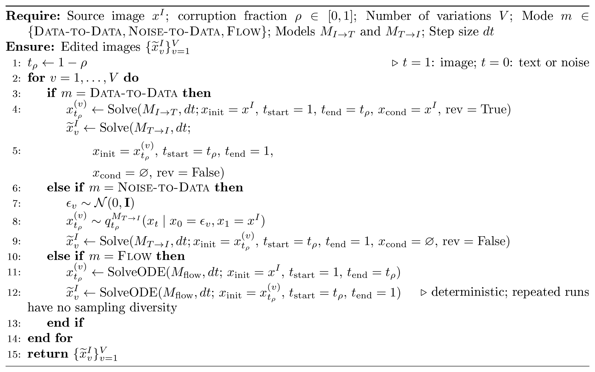
Algorithm 1 is printed for an image source. For a text source, set $t_\rho=\rho$, integrate the endpoint-conditioned forward model from $0$ to $t_\rho$, and then integrate the state-only reverse model from $t_\rho$ back to $0$; the noise-to-data construction is obtained by the same endpoint swap. The flow comparison uses the single unconditional field in both directions with the signed Euler update $x_{k+1}=x_k+(t_{k+1}-t_k)\widehat{u}(x_k, t_k)$.

L. Industrial-Scale Model Details

In Table 2, we compare our 1B model against foundation models. We evaluate the foundation models on the same testing set as our models.

Qwen-3-VL-4B-Instruct: This was used to generate the captions by the creators of the GPIC dataset ([21]). It is therefore a natural teacher/reference anchor for performance on this caption distribution, though not a mathematical upper bound under the reported evaluation metrics. Also, even our largest 1B model still has only a quarter of the parameters. As such, it is encouraging that the performance is as close as it is.

Stable Diffusion 1.5: This model uses the same VAE that we do. We used the community standard settings: CFG 7.5, 50 steps, and default settings from the HuggingFace pipeline ([3]).

M. Technical Details of Bridge-Based Image Editing

Setting.

Let $x_0$ denote a text state and $x_1$ an image latent, represented in the common tensor layout used by our data-to-data bridge. We require either one bidirectional bridge model or two direction-specific models sharing the same transport process. This experiment is specific to a data-to-data bridge because the text and image are themselves the two endpoints of the process.

Our implementation uses a driftless reference SDE ($A=0$), with scalar volatility $\sigma(t)$. The learned forward process is discretized by Euler–Maruyama as

$ X_{i+1}

X_i + \sigma(t_i)^2 s_\theta(X_i, t_i;x_0, y)\Delta t_i + \sigma(t_i)\Delta B_i,\tag{40} $

where $s_\theta$ is the learned forward score, $x_0$ is also supplied as the conditioning endpoint, and $y$ denotes the prompt-type label.

Inferring text from the source image.

Given a source-image latent $z$, we first integrate the reverse image-to-text bridge from $t=1$ to $t=0$, conditioned on $z$. The resulting continuous state may not correspond exactly to valid token embeddings, due to network approximation and discretization error. We therefore decode a token ID at each position using the model's token decoder (see Appendix H.2), infer the sequence length using the token-norm stopping criterion (norms close to zero are padding), and snap every retained position to its vocabulary-table embedding.

Specifically, if $\hat{\ell}_j$ is the decoded token at position $j$, its snapped embedding is

$ e_j

\rho \frac{V_{\hat{\ell}j}} {\lVert V{\hat{\ell}_j}\rVert_2},\tag{41} $

where $V$ is the vocabulary embedding table, and $\rho$ is the token scaling factor used during training. Positions after the inferred stopping point are set to zero. This produces both a discrete pseudo-caption and an on-manifold text endpoint $x_0^{(0)}$. No dataset caption is used by the editing pipeline.

Automated semantic editing.

We prompt an LLM to rewrite the inferred caption by replacing $k$ words while leaving the remainder unchanged. We sample several candidate responses and retain the one whose token-level difference is closest to the requested edit size. Thus, the LLM provides an automated and reproducible proxy for a human semantic edit; neither the particular LLM nor exact satisfaction of the requested number of word replacements is required by the bridge procedure.

The edited caption is tokenized using the same tokenizer (Qwen3-Embedding) used to generate the dataset, and re-embedded using the same normalized vocabulary table as in Equation 41. Let $e_j^{(0)}$ and $e_j^{(1)}$ denote unit-normalized embeddings at a token position in the original and edited captions. At interpolation coordinate $\lambda\in[0, 1]$, positions present in both sequences are interpolated along the unit sphere ([36]):

$ \begin{aligned} \omega_j &= \arccos!\left(\left\langle e_j^{(0)}, e_j^{(1)}\right\rangle \right), \ e_j^{(\lambda)} &= \frac{\sin((1-\lambda)\omega_j)}{\sin\omega_j}e_j^{(0)} + \frac{\sin(\lambda\omega_j)}{\sin\omega_j}e_j^{(1)}. \end{aligned}\tag{42} $

For numerical stability, whenever $|\sin\omega_j|$ is numerically small (below $10^{-6}$), we fall back to $e_j^{0}$. If a position occurs in only one sequence, its embedding magnitude is linearly faded out or in. The resulting embeddings are multiplied by $\rho$ and rearranged into the bridge tensor layout, producing text endpoints ${x_0^{(\lambda)}}_{\lambda\in\Lambda}$.

Noise backsolving.

Using independently sampled noise for each $\lambda$ would obscure the effect of the edit with unrelated changes in composition and layout. Instead, we construct a reference path from the unedited text endpoint $x_0^{(0)}$ to the source latent $z$ and infer the stochastic increments that make this path consistent with the learned discretized dynamics.

Let

$ C(a, b)=\int_a^b \sigma(s)^2, ds.\tag{43} $

Let $t_i = \frac{i}{N}$. For $t_i<t_{i+1}$, define $v_i=C(t_i, t_{i+1})$ and $V_i=C(t_i, 1)$. The conditional transition of the driftless reference bridge is (following Equation 14):

$ q_{\mathrm{ref}} \left(x_{i+1}\mid x_i, z \right)

\mathcal{N}\left(x_i+\frac{v_i}{V_i}(z-x_i), \left(v_i-\frac{v_i^2}{V_i}\right)\mathbf{I} \right).\tag{44} $

Sequentially sampling this transition gives a path $\bar{x}_0=x_0^{(0)}, \ldots, \bar{x}_N=z$.

For each step, we rearrange Equation 40 to infer its driving increment:

$ \widehat{\Delta B}_i

\frac{\bar{x}_{i+1}-\bar{x}_i}{\sigma(t_i)}

\sigma(t_i) s_\theta(\bar{x}_i, t_i;x_0^{(0)}, y)\Delta t_i.\tag{45} $

These quantities are best interpreted as backsolved driving residuals: because the reference path is sampled first and then reconciled with the learned drift, they need not be fresh independent Brownian draws. More precisely, the sampled reference path follows the endpoint-pinned base law $\mathbb{P}^{(x_0^{(0)}, z)}$, while replay uses the learned data-generating drift conditioned only on $x_0^{(0)}$. Equation 45 algebraically reconciles those two discretized dynamics; it is not a discretization of a change of measure between the unconditioned laws $\mathbb{P}$ and $\mathbb{Q}$ (cf. Equation 35 of [10]).

Require: Source latent $z$; original text $x_0^{(0)}$; edited text endpoints
$\{x_0^{(\lambda)}\}_{\lambda\in\Lambda}$; score $s_\theta$;
volatility $\sigma$; label $y$; grid $0=t_0<\cdots<t_N=1$
$\bar{x}_0 \gets x_0^{(0)}$
for $i=0,\ldots,N-1$ do
  Sample
  $\bar{x}_{i+1}\sim q_{\mathrm{ref}}(\cdot\mid\bar{x}_i,z)$
  using Eq. 44
  $\Delta t_i\gets t_{i+1}-t_i$
  $\displaystyle \widehat{\Delta B}_i\gets \frac{\bar{x}_{i+1}-\bar{x}_i}{\sigma(t_i)} - \sigma(t_i)s_\theta( \bar{x}_i,t_i;x_0^{(0)},y)\Delta t_i$
end for
for $\lambda\in\Lambda$ do
  $X_0^{(\lambda)}\gets x_0^{(\lambda)}$
  for $i=0,\ldots,N-1$ do
    $\displaystyle X_{i+1}^{(\lambda)} \gets X_i^{(\lambda)} + \sigma(t_i)^2 s_\theta( X_i^{(\lambda)},t_i;x_0^{(\lambda)},y)\Delta t_i + \sigma(t_i)\widehat{\Delta B}_i$
  end for
  $\hat{z}^{(\lambda)}\gets X_N^{(\lambda)}$
end for
Ensure: Structurally aligned edited latents
$\{\hat{z}^{(\lambda)}\}_{\lambda\in\Lambda}$

For $\lambda=0$, replay starts from the same text endpoint used during backsolving. Equation 45 therefore makes every replayed update equal to its corresponding reference-path update, recovering the source latent up to numerical precision. For $\lambda>0$, the initial state and score evaluations change, but the inferred driving increments remain fixed. Since these increments were obtained from a path anchored at the source image, replay tends to preserve its coarse spatial organization while allowing the edited text to alter semantic content.

Experimental configuration.

We use $N=400$ steps for both image-to-text inference and text-to-image generation, five evenly spaced interpolation angles including both caption endpoints, and classifier-free guidance scale zero. Every interpolation point for a given source reuses exactly the same inferred increment sequence from Equation 45. We decode the final latents with the pretrained image VAE and display each generated image together with the decoded text at its interpolation coordinate.

N. LARRY state-fate benchmark details

Metrics We evaluate both pointwise accuracy and distributional structure. Forward and reverse mean-squared error measure how well the model reconstructs paired descendant and progenitor states. RBF-MMD compares the generated and real cell-state distributions, testing whether the model matches the target population. Fate and clone kNN accuracy measure whether each generated cell is nearest to real cells with the correct fate label or lineage clone, which directly probes biological consistency. Finally, cycle-consistency error evaluates whether a generated descendant can be mapped back to its original progenitor, and vice versa. Together, these metrics separate models that merely generate plausible cells from ones that preserve lineage-resolved state-fate relationships.

Dataset Processing We construct clone-paired endpoint examples from the in vitro LARRY lineage-tracing dataset by pairing day-2 progenitor cells with day-6 descendant cells that share the same lineage barcode. We preprocess normalized counts by selecting the top 2, 000 highly variable genes and projecting cells to a 64-dimensional latent representation using TruncatedSVD. For each eligible clone, we sample up to 32 day-2/day-6 endpoint pairs and split data by clone into train, validation, and test partitions, preventing lineage leakage across splits. The resulting benchmark contains 31, 840 training pairs and 3, 968 evaluation pairs.

Architecture All compared neural methods use the same vector DiT backbone unless otherwise stated. The model tokenizes the 64-dimensional cell latent into 8-dimensional tokens, embeds them with width 768, and applies 12 transformer blocks with 12 attention heads and AdaLN-style conditioning. The conditioning vector includes the bridge time, the experimental/context label, a forward/reverse direction embedding, and the source endpoint state. The shared BIT model uses one bidirectional network for both day-2 $\to$ day-6 and day-6 $\to$ day-2 transport; the separate-model ablation uses independent networks for the two directions.

Training Details We train all models for 20, 000 optimization steps with AdamW, learning rate 2 x 10^-4, batch size 512, gradient clipping at 1.0, and bfloat16 mixed precision. Score-based bridges are sampled with 250 SDE steps. The main BIT model uses the uniform-volatility bridge with $K=0.5$; the cosine baseline uses a cosine-decay volatility schedule with $\epsilon=0.03$; the rectified-flow baseline uses the same DiT architecture with a flow-matching objective; and endpoint regression directly predicts the target endpoint from the source endpoint.

O. Training Pseudocode

See Algorithm 3.

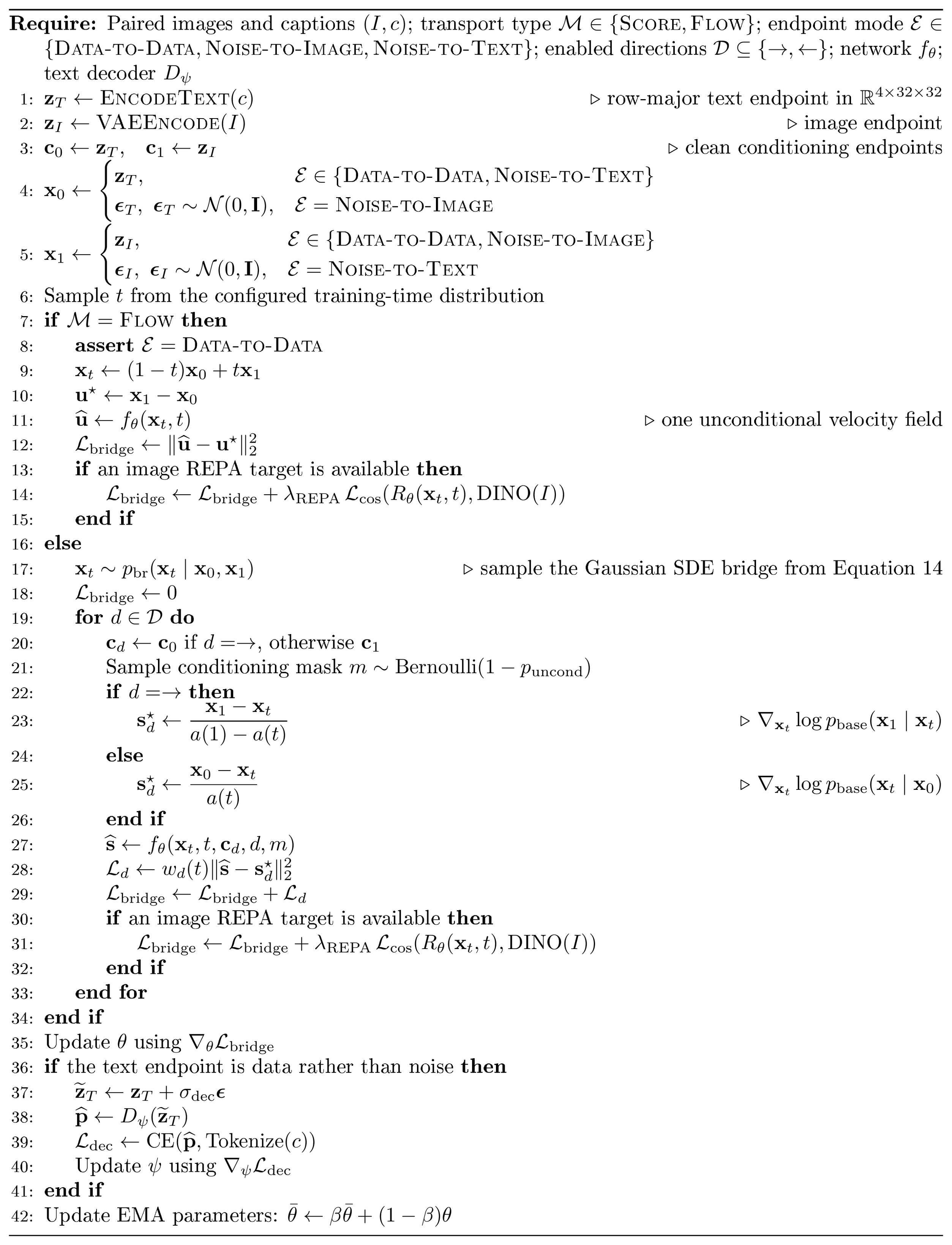
P. Inference Pseudocode

See Algorithm 4.

Require: Source $a$; direction $d\in\{\rightarrow,\leftarrow\}$;
transport type $\mathcal{M}$
EMA network $f_{\bar{\theta}}$;
integration steps $N$; guidance strength $\gamma$
$\Delta t\gets1/N$
if $d=\rightarrow$ // Text-to-Image then
  $\mathbf{c}\gets\operatorname{EncodeText}\left(a\right)$
  $\mathbf{x}\gets \mathbf{c}$ for data-to-data transport, otherwise
  $\mathbf{x}\sim\mathcal{N}(0,\mathbf{I})$
  $\rho\gets+1$
else
  $\mathbf{c}\gets\operatorname{VAEEncode}\left(a\right)$
  $\mathbf{x}\gets \mathbf{c}$ for data-to-data transport, otherwise
  $\mathbf{x}\sim\mathcal{N}(0,\mathbf{I})$
  $\rho\gets-1$
end if
for $n=0,\ldots,N-1$ do
  $u_n\gets n/N$
  $t_n\gets u_n$ if $d=\rightarrow$, otherwise $t_n\gets1-u_n$
  // $u_n$: integration time; $t_n$: network time
  if $\mathcal{M}=\textsc{Flow}$ then
    $\widehat{\mathbf{u}}\gets f_{\bar{\theta}}(\mathbf{x},t_n)$
    // single unconditional field
    $\mathbf{x}\gets \mathbf{x}+\rho\,\Delta t\,\widehat{\mathbf{u}}$
  else
    $\mathbf{s}_{c}\gets f_{\bar{\theta}}(\mathbf{x},t_n,\mathbf{c},d, \mathrm{conditioned})$
    if $\gamma>0$ then
      $\mathbf{s}_{u}\gets f_{\bar{\theta}}(\mathbf{x},t_n,\mathbf{c},d, \mathrm{unconditioned})$
      $\widehat{\mathbf{s}}\gets \mathbf{s}_{c}+ \gamma(\mathbf{s}_{c}-\mathbf{s}_{u})$
    else
      $\widehat{\mathbf{s}}\gets\mathbf{s}_{c}$
    end if
    Sample $\boldsymbol{\epsilon}\sim\mathcal{N}(0,\mathbf{I})$
    $\mathbf{x}\gets\mathbf{x} +\sigma(t_n)^2\widehat{\mathbf{s}}\,\Delta t +\sigma(t_n)\sqrt{\Delta t}\,\boldsymbol{\epsilon}$
    // Euler--Maruyama bridge step
  end if
end for
// The finite- $N$ output is a discretization approximation, not an endpoint-exact draw.
if $d=\rightarrow$ then
  $\widehat{I}\gets \operatorname{VAEDecode}\left(\mathbf{x}\right)$
  return $\widehat{I}$
else
  $(\mathbf{E}_{1},\ldots,\mathbf{E}_{64}) \gets\operatorname{UnpackTextVectors}\left(\mathbf{x}\right)$
  // vectors before decoder normalization
  $\widehat{\mathbf{k}}\gets \arg\max D_{\psi}(\mathbf{E}_{1:64})$
  $\ell\gets \min{i:\|\mathbf{E}_{i}/\rho_{\mathrm{tok}}\|_{2}<0.1}$
  // $\rho_{\mathrm{tok}}$: training-time token scale
  return
  $\operatorname{QwenDecode}\left(\widehat{\mathbf{k}}_{1:\ell-1}\right)$
end if

Q. Large-Scale Model Hyperparameters

To see how far we can push the performance, we also train a larger model with more compute resources. Overall, it is an improvement (compare Table 2's results in row $\omega=0.0$ to Table 1).

Changed Settings: The large-scale model uses DiTXA-XL/2, comprising 28 transformer blocks with hidden dimension 1152, 16 attention heads, and $2\times2$ patches. This results in $1, 054, 621, 840$ parameters. (This is larger than the DiTXA-L/2 backbone used in the controlled comparisons, which has 24 blocks and hidden dimension 1024.) The large-scale model is trained jointly in both the text-to-image and image-to-text directions: each batch produces one loss for each direction, and the two losses are summed before a single optimizer update.

Endpoint conditioning is dropped with probability 0.1, compared with 0.3 for the controlled score-model ablations. Image REPA is applied from the beginning of training at transformer layer 8 with weight 0.75 (the controlled image-generating models use the same layer and schedule but a smaller weight of 0.5). We train the large-scale model for 122, 500 steps with a global batch size of 1792 (compared with 200, 000 steps and a batch size of 512 in the controlled comparisons). This corresponds to approximately twice as many training examples as the ablation models saw. Optimization uses AdamW with learning rate 2.5 x 10^-4, larger than the controlled-model rate of 1.5 x 10^-4; this value was selected for the larger-batch run rather than obtained by a stated linear-scaling rule.

Kept Settings: The things that stay the same are the AdamW $(\beta_1, \beta_2)=(0.9, 0.999)$, zero weight decay, gradient clipping at 1.0, 5, 000 steps of linear warm-up followed by a constant learning rate, and primary EMA decay of 0.9995. The large-scale model also uses the same periodic bridge SDE with $\alpha=0.95, k=1.0, \epsilon_{\mathrm{SDE}}=0.05$. These parameters match the periodic-SDE arm of the main text experiments. Bridge times are sampled from a logit-normal distribution with mean 0.4 and standard deviation 0.7 (as opposed to the uniform time sampling in the main text ablation experiments), clipped to $[9.9\times10^{-4}, 1-9.9\times10^{-4}]$. The DINOv2 targets, token-bridge construction, row-major text layout, dataset, VAE representation, and token-decoder design are otherwise unchanged.

Training is distributed over 16 compute nodes with four NVIDIA A100 80 GB GPUs per node, for 64 GPUs in total. The controlled comparisons use two nodes and eight GPUs.

R. Image Editing Along Text–Image Bridges

We use our text–image bridges to construct an end-to-end image editing procedure that exposes editing trajectories native to the learned bridge. Given only a source image, we first traverse the bridge in the reverse direction, from image to text, to infer a textual description. We then modify the inferred description and traverse the bridge forward, using the same implied noise, to generate an edited image. In our experiments, an LLM (which we use as an automated proxy for human edits) is prompted to replace a small number of words while preserving the remainder of the sentence. Both the original and edited descriptions are embedded using the bridge's vocabulary table, and we form a continuous path between them using token-wise spherical interpolation to get a spectrum of edits. Overall, this experiment illustrates a distinctive capability of text–image bridges: an image can be inverted into an editable semantic representation and then transported back through a continuous family of structurally aligned image edits. See Figure 4 for qualitative results, and Appendix M for setup.

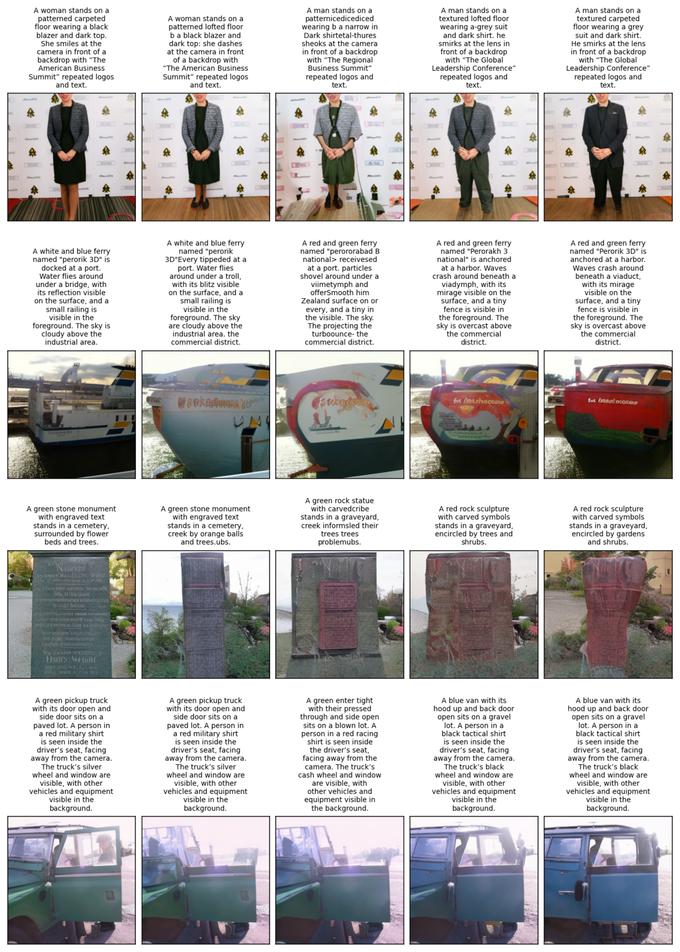
S. Impact of REPA on Image-to-Text Generation

REPA ([32]) has been known to greatly improve image generation quality. Surprisingly, we find that using REPA with image features can also help the image-to-text generation in our BIT framework. In particular, for only a slight hit in generative perplexity, we see a large boost in CLIP score. We think this is because the REPA loss forces the generated text to align with the image's semantic content, but at the cost of missing some fine syntactical details. See Table 4.

\begin{tabular}{lcc}
  \toprule
  Method & Gen PPL ($\downarrow$) & CLIP ($\uparrow$) \\
  \midrule
  \textbf{\texttt{BIT}} (without REPA) & 112.7 & 22.7 \\
  \textbf{\texttt{BIT}} (REPA $\lambda=0.5$) & 123.4 & 27.0 \\
  \bottomrule
  \end{tabular}

T. Qualitative Cross-Modal Round-Trip Stochastic Variation Results

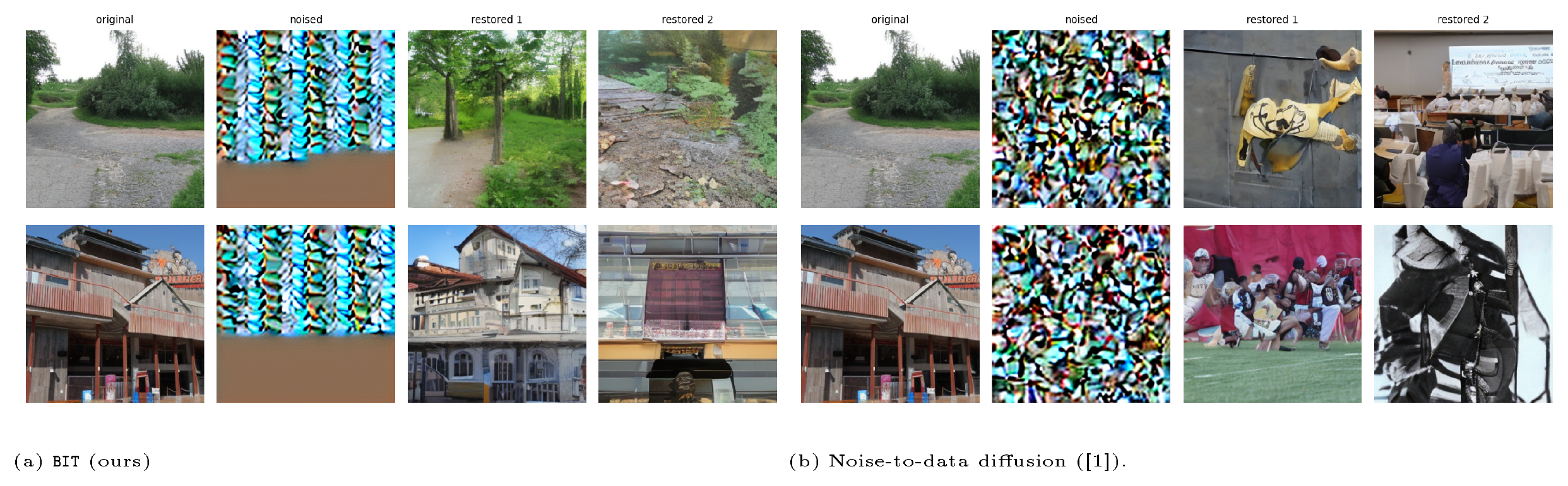
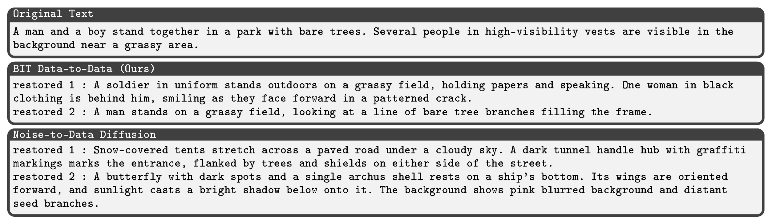
U. Related Works

Diffusion Bridges: Our work builds on the rich literature in diffusion bridge models, which generalize diffusion models by learning SDEs that interpolate between data distributions (rather than from noise to data) to model conditional distributions ([11, 10, 25]). DDBM ([11]) is equivalent to the reverse-time SDE of our framework (Theorem 2), but does not consider the forward-time or marginal SDEs and is therefore unidirectional. Our forward-time SDE (Theorem 1) is a special case of ABC ([10]); unlike that work, we also consider the reverse-time SDE so that we can sample either conditional distribution. BDBM ([25]) is the closest to our framework in that they also construct bidirectional models, but their derivations come from the perspective of Chapman-Kolmogorov equations on Gaussian distributions rather than our measure-theoretic perspective on SDEs. They also do not consider the marginal/unconditional transitions, which precludes their ability to do techniques like classifier-free guidance. Crucially, none of the previous diffusion bridge papers even attempt text-to-image translation, mostly sticking to translation between observations from the same modality, like image-to-image.

Data-to-Data Flow: Flow matching with coupled distributions has been proposed as a way to translate directly between different modalities, e.g., image and text. The main problem is that the flow matching ODE is deterministic, so in a bare-bones implementation, it inherently cannot express the myriad of possibilities in the conditional distribution. To get around this, there is a variety of hacks proposed in previous works. FlowTok ([20]) and CrossFlow ([22]) learn variational encoders ([37]) to map text and image into a common domain: crucially, the noise introduced by the variational encoders breaks the inherent determinism of flows, enabling some semblance of stochasticity rather than blurred average predictions. However, the success of their method hinges on careful tuning and training tricks for their encoders that are somewhat specific to the text-to-image domain, e.g., auxiliary contrastive learning with CLIP embeddings. Their framework, as it currently stands, is not clearly applicable out-of-the-box to other domains, while ours is. [19] also addresses data-to-data translation with flows, albeit for tasks such as superresolution and inpainting rather than text-to-image. Their solution to the lack of stochasticity is to perturb source samples with Gaussian noise. This modification removes a clear deterministic reverse mapping when generating in the opposite direction.

Cycle-Consistent Generative Models: CycleGAN ([9]) also addresses bidirectional translation between domains with a cycle-consistency loss and a GAN loss, but they model it as a deterministic process, which is inherently incorrect. BDBM ([25]), as discussed earlier, has bidirectional capabilities, and they correctly model the translation as stochastic.

Continuous Diffusion for Language: Recently, there has been interest in methods for continuous-time, continuous-space processes to generate language. Embedded Language Flows ([5]) has a similar solution to ours, in that they use invertible text token embeddings as the target distribution for a flow matching model. However, they only consider single-modality generation (no image conditioning or generation), and still use the basic construction of Gaussian noise-to-data. Flow Map Language Models [26] and Discrete Flow Maps ([27]) learn few-step generators for one-hot token vectors via cross-entropy and consistency losses. Again, they do not consider multimodality tasks like text-to-image.

Text-to-Image: Text-to-image models are ubiquitous, having moved past the academic sphere to products like Midjourney. However, the dominant research ecosystem models are Flux ([4]) and Stable Diffusion ([3]). They are generally based on noise-to-data conditional diffusion or flow. They are also not invertible, unlike our framework.

References

Section Summary: This section lists dozens of academic papers, preprints, and a few classic books that the authors drew upon for their work. Most focus on modern AI techniques for generating and editing images using diffusion models, flow matching, and related stochastic methods, often combining them with language models or visual instruction data. A smaller number cover foundational mathematics in probability and stochastic processes, along with supporting tools for evaluation and representation learning.

[1] Song et al. (2020). Score-based generative modeling through stochastic differential equations. arXiv preprint arXiv:2011.13456.

[2] Albergo et al. (2025). Stochastic interpolants: A unifying framework for flows and diffusions. Journal of Machine Learning Research. 26(209). pp. 1–80.

[3] Rombach et al. (2022). High-resolution image synthesis with latent diffusion models. In Proceedings of the IEEE/CVF conference on computer vision and pattern recognition. pp. 10684–10695.

[4] Labs et al. (2025). FLUX. 1 Kontext: Flow Matching for In-Context Image Generation and Editing in Latent Space. arXiv preprint arXiv:2506.15742.

[5] Hu et al. (2026). ELF: Embedded Language Flows. arXiv preprint arXiv:2605.10938.

[6] Meng et al. (2021). Sdedit: Guided image synthesis and editing with stochastic differential equations. arXiv preprint arXiv:2108.01073.

[7] Bai et al. (2025). Qwen3-vl technical report. arXiv preprint arXiv:2511.21631.

[8] Liu et al. (2023). Visual instruction tuning. Advances in neural information processing systems. 36. pp. 34892–34916.

[9] Zhu et al. (2017). Unpaired image-to-image translation using cycle-consistent adversarial networks. In Proceedings of the IEEE international conference on computer vision. pp. 2223–2232.

[10] Guo et al. (2026). ABC: Any-Subset Autoregression via Non-Markovian Diffusion Bridges in Continuous Time and Space. arXiv preprint arXiv:2604.27443.

[11] Zhou et al. (2023). Denoising diffusion bridge models. arXiv preprint arXiv:2309.16948.

[12] Girsanov, Igor Vladimirovich (1960). On transforming a certain class of stochastic processes by absolutely continuous substitution of measures. Theory of Probability & Its Applications. 5(3). pp. 285–301.

[13] Doob, Joseph L and others (1984). Classical potential theory and its probabilistic counterpart. Springer.

[14] Yang et al. (2025). Qwen3 technical report. arXiv preprint arXiv:2505.09388.

[15] Peebles, William and Xie, Saining (2023). Scalable diffusion models with transformers. In Proceedings of the IEEE/CVF international conference on computer vision. pp. 4195–4205.

[16] Ho, Jonathan and Salimans, Tim (2022). Classifier-free diffusion guidance. arXiv preprint arXiv:2207.12598.

[17] Zhang et al. (2025). Qwen3 embedding: Advancing text embedding and reranking through foundation models. arXiv preprint arXiv:2506.05176.

[18] Kusupati et al. (2022). Matryoshka representation learning. Advances in Neural Information Processing Systems. 35. pp. 30233–30249.

[19] Albergo et al. (2023). Stochastic interpolants with data-dependent couplings. arXiv preprint arXiv:2310.03725.

[20] He et al. (2025). Flowtok: Flowing seamlessly across text and image tokens. In Proceedings of the IEEE/CVF International Conference on Computer Vision. pp. 16629–16640.

[21] Chandrasegaran et al. (2026). Gpic: A giant permissive image corpus for visual generation. arXiv preprint arXiv:2605.30341.

[22] Liu et al. (2025). Flowing from words to pixels: A noise-free framework for cross-modality evolution. In Proceedings of the Computer Vision and Pattern Recognition Conference. pp. 2755–2765.

[23] Midjourney (2026). Variations. https://docs.midjourney.com/hc/en-us/articles/32692978437005-Variations.

[24] Caleb Weinreb et al. (2020). Lineage tracing on transcriptional landscapes links state to fate during differentiation. Science. 367(6479).

[25] Kieu et al. (2025). Bidirectional diffusion bridge models. In Proceedings of the 31st ACM SIGKDD Conference on Knowledge Discovery and Data Mining V. 2. pp. 1139–1148.

[26] Lee et al. (2026). Flow map language models: One-step language modeling via continuous denoising. arXiv preprint arXiv:2602.16813.

[27] Potaptchik et al. (2026). Discrete flow maps. arXiv preprint arXiv:2604.09784.

[28] Øksendal, Bernt (2003). Stochastic differential equations.

[29] Anderson, Brian DO (1982). Reverse-time diffusion equation models. Stochastic Processes and their Applications. 12(3). pp. 313–326.

[30] Trevisan, Dario (2016). Well-posedness of multidimensional diffusion processes with weakly differentiable coefficients. Electronic Journal of Probability. 21(22). pp. 1–41. doi:10.1214/16-EJP4453.

[31] Cover, Thomas M (1999). Elements of information theory. John Wiley & Sons.

[32] Yu et al. (2024). Representation alignment for generation: Training diffusion transformers is easier than you think. arXiv preprint arXiv:2410.06940.

[33] Heusel et al. (2017). Gans trained by a two time-scale update rule converge to a local nash equilibrium. Advances in neural information processing systems. 30.

[34] Radford et al. (2021). Learning transferable visual models from natural language supervision. In International conference on machine learning. pp. 8748–8763.

[35] Oquab et al. (2023). Dinov2: Learning robust visual features without supervision. arXiv preprint arXiv:2304.07193.

[36] Matthias Geier (2026). Spherical Linear Interpolation (Slerp). https://splines.readthedocs.io/en/latest/rotation/slerp.html.

[37] Kingma, Diederik P and Welling, Max (2013). Auto-encoding variational bayes. arXiv preprint arXiv:1312.6114.