The good, the bad and the ugly sides of data augmentation: An implicit spectral regularization perspective

Chi-Heng LinChiraag KaushikEva L. DyerVidya Muthukumar

article2024JMLR56 citations

Establishes a theoretical framework that reveals how data augmentation acts as implicit spectral regularization by reshaping the covariance spectrum and adding ridge penalty, explaining why common augmentations can either aid or harm generalization across underparameterized and overparameterized regimes.

Listen

Modern machine learning systems rely extensively on data augmentation—the practice of applying stochastic transformations such as random masking, cutout, or noise injection to training data—to prevent overfitting and boost generalization. While classical theory assumed augmentations simply generate new samples from the original data distribution, modern techniques intentionally and drastically alter the underlying distribution. Until now, practitioners lacked a unified theoretical foundation to explain exactly how, why, and when these out-of-distribution transformations succeed or fail. The article's primary objective is to establish a quantitative, non-asymptotic framework that characterizes the impact of general stochastic data augmentations on generalization across underparameterized and overparameterized linear models in both regression and classification tasks.

To evaluate these dynamics, the authors developed a mathematical framework that maps augmented empirical risk minimization directly to an equivalent ridge regression problem with a modified data spectrum. The analysis separates the effect of data augmentation into explicit variance regularization and implicit data covariance manipulation. The authors established a deterministic approximation proving that high-dimensional sample correlations introduced by augmentations remain mathematically negligible for major augmentation families. They derived closed-form generalization bounds for canonical augmentations—including Gaussian noise injection, random masking, cutout, and salt-and-pepper noise—and introduced a novel random-rotation augmentation method. The theoretical findings were corroborated through extensive numerical experiments comparing closed-form solutions with practical augmented stochastic gradient descent across varying sample sizes, dimensions, and noise levels.

The analysis identified several critical findings regarding model performance. First, data augmentation inherently reduces model variance by uniformly boosting the data spectrum, effectively smoothing out and eliminating the sharp error spikes associated with the double descent phenomenon near the interpolation threshold. Second, popular techniques such as random masking and cutout act by flattening or isotropizing the data spectrum; this trade-off reduces variance at the expense of increasing bias, which benefits classification and underparameterized regression but can severely degrade performance in overparameterized regression. Third, augmentations that are biased on average induce distribution shifts that penalize regression accuracy through covariate and label shift, whereas classification tasks remain largely immune to these biases as long as the underlying signal direction is preserved. Fourth, the authors' proposed random-rotation augmentation successfully achieves variance reduction comparable to ridge regression while maintaining the minimal bias of least-squares estimation.

These insights show that data augmentation strategies cannot be applied as one-size-fits-all solutions. In classification tasks and moderately dimensioned regimes, variance reduction dominates, making aggressive stochastic augmentation highly effective and robust to hyperparameter tuning. In contrast, high-dimensional regression requires careful preservation of low-rank data structures, where uncalibrated augmentations can inadvertently destroy semantic information and degrade test performance. Practitioners should prioritize on-the-fly augmentation over static pre-computation, as dynamic sampling steadily suppresses variance without creating artificial interpolation bottlenecks. Furthermore, data teams deploying augmentations for regression must ensure transformations are mean-unbiased and preferentially target noise features over predictive signal features.

The conclusions are supported with high mathematical rigor and tight non-asymptotic bounds for sub-Gaussian linear models. However, the study's primary limitation is its focus on linear and kernel-based architectures under squared loss. Stakeholders should exercise caution when extrapolating these precise spectral regularization dynamics directly to highly non-linear deep neural networks or self-supervised representation pipelines without conducting preliminary empirical validations.

Georgia Institute of Technology boosting classification methods computer vision implicit spectral regularization data augmentation data-dependent regularization

arXiv: 2210.05021 nerdslab/augmentation-theory

No sufficiently relevant recommendations were found.

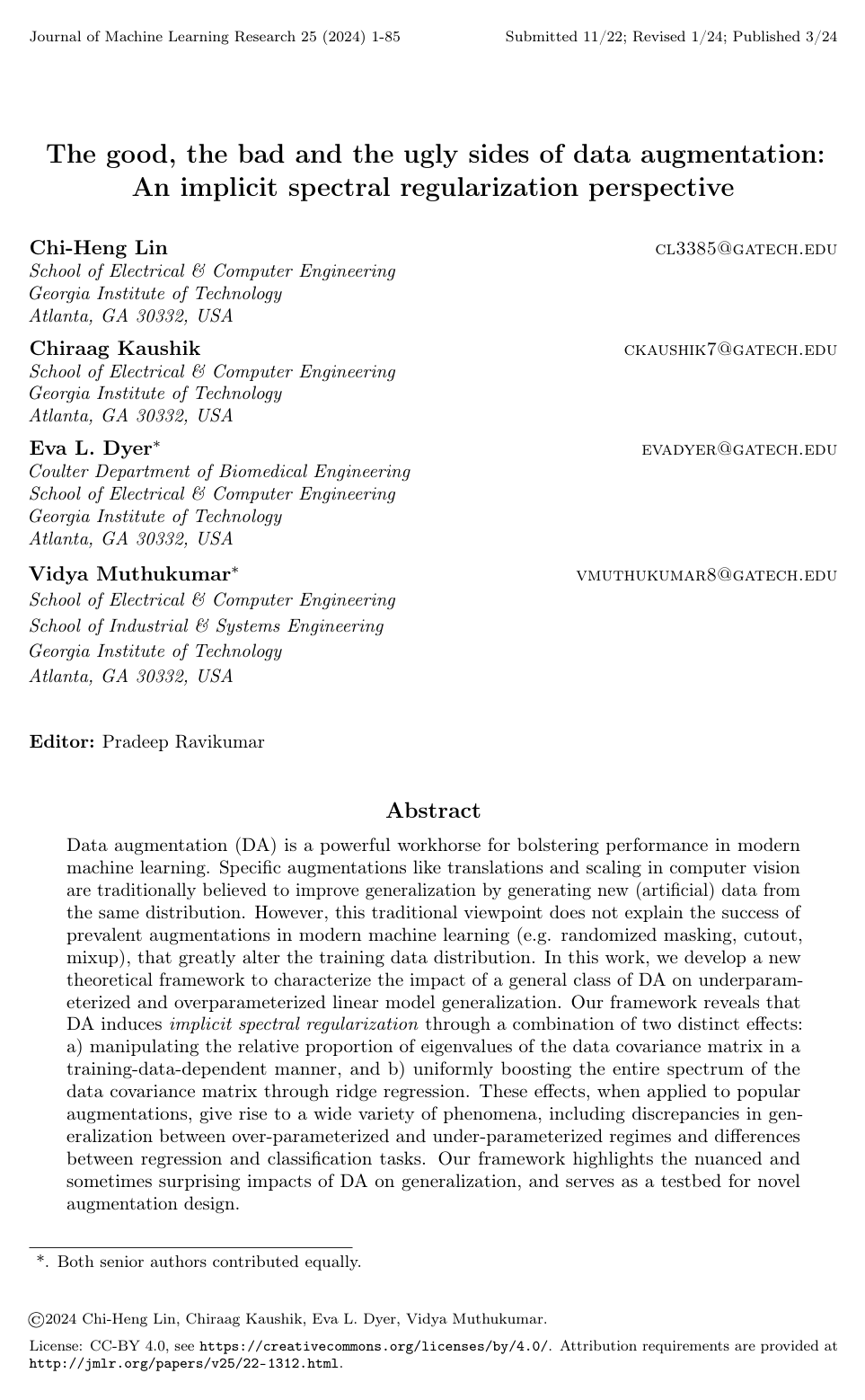
Cover for The good, the bad and the ugly sides of data augmentation: An implicit spectral regularization perspective

Abstract

Data augmentation (DA) is a powerful workhorse for bolstering performance in modern machine learning. Specific augmentations like translations and scaling in computer vision are traditionally believed to improve generalization by generating new (artificial) data from the same distribution. However, this traditional viewpoint does not explain the success of prevalent augmentations in modern machine learning (e.g. randomized masking, cutout, mixup), that greatly alter the training data distribution. In this work, we develop a new theoretical framework to characterize the impact of a general class of DA on underparameterized and overparameterized linear model generalization. Our framework reveals that DA induces implicit spectral regularization through a combination of two distinct effects: a) manipulating the relative proportion of eigenvalues of the data covariance matrix in a training-data-dependent manner, and b) uniformly boosting the entire spectrum of the data covariance matrix through ridge regression. These effects, when applied to popular augmentations, give rise to a wide variety of phenomena, including discrepancies in generalization between over-parameterized and under-parameterized regimes and differences between regression and classification tasks. Our framework highlights the nuanced and sometimes surprising impacts of DA on generalization, and serves as a testbed for novel augmentation design.

1. Introduction
1.1 Main contributions
1.2 Notation
2. Related Work
2.1 Data augmentation
2.2 Interpolation and regularization in overparameterized models
3. Problem Setup
3.1 Empirical risk minimization with data augmentation
3.2 Implications of a DA-induced regularizer and connections to ridge regression
3.3 Application to different augmentations used in practice
4. Main Results
4.1 Preliminaries
4.1.1 Error Metrics
4.1.2 Spectral quantities of interest
4.2 A deterministic approximation strategy for DA analysis
4.3 Regression analysis
4.3.1 Regression analysis for general classes of unbiased augmentations
4.3.2 Regression analysis for general biased-on-average augmentations
4.4 Classification analysis
4.4.1 Classification analysis setup
4.4.2 Classification analysis for unbiased-on-average augmentations
4.4.3 Classification analysis for general biased-on-average augmentations
4.5 Classes of augmentations for which our theory applies
5. Case Studies: Applying Our Theory to Study Different Classes of DA
5.1 Gaussian noise injection
5.2 Randomized masking
5.2.1 Feature-adaptive random masking
5.3 Random cutout
5.4 Composite augmentation: Salt-and-pepper
5.5 A new 'random-rotation' augmentation
6. Experiments
6.1 Convergence of aSGD to the closed-form aERM solution
6.2 Comparisons of different types of augmentations
6.3 Studying the interactions between the original covariance and augmentations
6.4 Comparisons of pre-computing samples vs. augmented ERM
7. The good, the bad and the ugly sides of data augmentation
7.1 The good: when DA helps generalization
7.2 The bad: when DA hurts generalization
7.3 The ugly: discrepancies in DA's effect under multiple factors
8. Conclusions and Future Work
Acknowledgements
Appendix
Appendix A. General Auxiliary Lemmas
Appendix B. Proofs of Regression Results
B.1 Regression Lemmas
B.2 Proof of Theorem 4
B.3 Proof of Theorem 7
B.4 Proof of Proposition 12
B.5 Proof of Proposition 13
B.6 Proof of Proposition 14
B.7 Proofs of Corollaries
Appendix C. Proofs of Classification Results
C.1 Classification Lemmas
C.2 Proof of Theorem 9
C.3 Proof of Theorem 11
C.4 Proofs of Corollaries
Appendix D. Comparisons between Regression and Classification
D.1 Proof of Proposition 46
D.2 Classification/regression separation for non-uniform random mask
Appendix E. Derivations of Common Augmented Estimators
Appendix F. Approximation Error for Dependent Feature Augmentation
F.1 Approximation error of random rotations
F.2 Approximation error of random cutout
Appendix G. Additional experiments
G.1 The implicit bias of minimal or 'weak' DA
References

Knowls

Knowl 1 — Stochastic augmentation is data-dependent Tikhonov regularization
model/method
Let $X\in\mathbb{R}^{n\times p}$ contain $n$ training examples as rows, let $y\in\mathbb{R}^n$ be their responses, and fit a linear predictor $x\mapsto x^\top\theta$ with squared loss. For an augmentation $g$ drawn randomly from a distribution $G$ , define its pointwise mean and covariance by $\mu_G(x)=\mathbb{E}_G[g(x)]$ and $\operatorname{Cov}_G(x)=\mathbb{E}_G[(g(x)-\mu_G(x))(g(x)-\mu_G(x))^\top]$ . The empirical augmentation covariance is $C_G(X)=n^{-1}\sum_{i=1}^n\operatorname{Cov}_G(x_i)$ , and $\mu_G(X)$ stacks the transformed means for the training examples.

The expected augmented empirical risk is
$\mathbb{E}_G\!\left[\|G(X)\theta-y\|_2^2\right] =\|\mu_G(X)\theta-y\|_2^2+n\theta^\top C_G(X)\theta.$
Thus stochastic augmentation contributes an explicit quadratic penalty whose matrix depends on the training data. When the augmentation is unbiased on average, meaning $\mu_G(x)=x$ , the first term is the ordinary least-squares loss. If $C_G(X)$ is positive definite, the resulting estimator is $\hat\theta_{\rm aug}=(X^\top X+nC_G(X))^{-1}X^\top y$ .

For a fixed covariance matrix $C$ , this estimator has the same prediction risk as ridge regression with transformed data $\widetilde X=XC^{-1/2}$ , transformed target parameter $C^{1/2}\theta^*$ , and ridge penalty $nI_p$ . In the original coordinates, augmentation therefore has two effects: it adds an $\ell_2$ -type regularization scale proportional to sample size $n$ , and changes the effective data covariance from $\Sigma$ to $C^{-1/2}\Sigma C^{-1/2}$ . In practice $C_G(X)$ depends on $X$ , so the fixed- $C$ ridge correspondence is approximate for general stochastic augmentations.
Knowl 2 — Finite-sample regression risk is governed by the augmentation-modified spectrum
theoretical result
Assume training covariates $x_i\in\mathbb{R}^p$ are i.i.d. with covariance $\Sigma$ , admit a sub-Gaussian representation $x=\Sigma^{1/2}z$ with isotropic $z$ , and responses follow $y_i=x_i^\top\theta^*+\epsilon_i$ with independent, zero-mean sub-Gaussian noise. Consider an augmentation unbiased on average, and let $C=\mathbb{E}_x[\operatorname{Cov}_G(x)]$ be positive definite. Define the transformed covariance and signal as $\Sigma_{\rm aug}=C^{-1/2}\Sigma C^{-1/2}$ and $\theta^*_{\rm aug}=C^{1/2}\theta^*$ . Write the eigenvalues of $\Sigma_{\rm aug}$ in descending order as $\lambda_1^{\rm aug},\ldots,\lambda_p^{\rm aug}$ , and let $P_{1:k}$ and $P_{k+1:p}$ project onto its first $k$ and remaining eigenspaces.

For a covariance with eigenvalues $\lambda_i$ , sample size $n$ , ridge scale $c$ , and index $k$ , define effective ranks
$\rho_k(\Sigma;c)=\frac{c+\sum_{i>k}\lambda_i}{n\lambda_{k+1}}, \qquad R_k(\Sigma;c)=\frac{(c+\sum_{i>k}\lambda_i)^2}{\sum_{i>k}\lambda_i^2}.$
Use $\rho_k^{\rm aug}=\rho_k(\Sigma_{\rm aug};n)$ and $R_k^{\rm aug}=R_k(\Sigma_{\rm aug};n)$ . Let $\Delta_G=\|C^{-1/2}C_G(X)C^{-1/2}-I_p\|_{\rm op}$ measure the discrepancy between empirical and population augmentation covariance, and let $\kappa$ be the condition number of $\Sigma_{\rm aug}$ . Under the paper’s bounded-condition-number assumptions on the residual Gram matrices and with $\Delta_G<c<1$ , the high-probability MSE of the augmented estimator is bounded, up to constants, by bias plus variance plus approximation error:
$\operatorname{MSE}(\hat\theta_{\rm aug})\lesssim B+V+E,$ $B\lesssim L_1^4\left[\|P_{k_1+1:p}\theta^*_{\rm aug}\|_{\Sigma_{\rm aug}}^2+ \|P_{1:k_1}\theta^*_{\rm aug}\|_{\Sigma_{\rm aug}^{-1}}^2 \frac{(\rho_{k_1}^{\rm aug})^2}{(\lambda_{k_1+1}^{\rm aug})^{-2}+(\lambda_1^{\rm aug})^{-2}(\rho_{k_1}^{\rm aug})^2}\right], \qquad V\lesssim L_2^2\left(\frac{k_2}{n}+\frac{n}{R_{k_2}^{\rm aug}}\right)\log n,$ $E\lesssim \kappa^{1/2}\Delta_G\left(\|\theta^*\|_{\Sigma}+\sqrt{B+V}\right).$
Here $\|v\|_A^2=v^\top Av$ , $k_1,k_2$ are spectral split indices, and $L_1,L_2$ bound the relevant residual-matrix condition numbers. The bound holds with high probability when the stated conditions hold. The bias and variance are controlled by the effective ranks of the transformed spectrum, not just the original data spectrum; $\Delta_G$ quantifies the additional error from replacing the random augmentation covariance with its population mean. The paper’s convergence assumption takes $p$ to grow polynomially with $n$ and requires $\Delta_G\to0$ ; several augmentation families have rates of order $\sqrt{\log n/n}$ .
Knowl 3 — Classification risk depends on signal survival relative to feature contamination
theoretical result
For the classification analysis, suppose labels are generated from a one-coordinate signal $\theta^*=\lambda_t^{-1/2}e_t$ : the label is $\operatorname{sgn}(x_t)$ , flipped independently with probability $\nu^*<1/2$ . Assume sub-Gaussian covariates with a bounded density, and that the signal feature is independent of the other features and their augmentations. The estimator is trained on binary labels using squared loss.

For any fitted coefficient vector $\hat\theta$ , define signal survival and noise contamination by
$\operatorname{SU}(\hat\theta)=\sqrt{\lambda_t}\,\hat\theta_t, \qquad \operatorname{CN}(\hat\theta)=\left(\sum_{j\ne t}\lambda_j\hat\theta_j^2\right)^{1/2}.$
Under the theorem’s spectral and residual-condition-number assumptions, and when replacing the sample augmentation covariance by its population mean changes the estimator by no more than the survival and contamination scales, the probability of classification error obeys
$\operatorname{POE}(\hat\theta)\lesssim \frac{\operatorname{CN}(\hat\theta)}{\operatorname{SU}(\hat\theta)} \left(1+\sigma_z\sqrt{\log\frac{\operatorname{SU}(\hat\theta)}{\operatorname{CN}(\hat\theta)}}\right),$
where $\sigma_z$ is the sub-Gaussian norm of the whitened covariates. For Gaussian covariates with independent features, the error has the exact form
$\operatorname{POE}(\hat\theta)=\frac12-\frac1\pi\tan^{-1}\!\left(\frac{\operatorname{SU}(\hat\theta)}{\operatorname{CN}(\hat\theta)}\right).$
The theorem bounds survival from below and above using the augmented signal eigenvalue and the effective rank $\rho_k(\Sigma_{\rm aug};n)$ ; contamination is controlled by a variance-like term involving $k/n+n/R_k$ for the spectrum with the signal coordinate removed. Thus good classification requires survival to dominate contamination. Unlike regression MSE, the 0–1 classification metric can tolerate substantial coefficient bias when the signal-to-contamination ratio remains favorable. The result requires the signal coordinate to lie among the leading augmented directions, with its index at most the sample size.
Knowl 4 — Mean-biased augmentation adds covariate-shift and label-shift penalties in regression
theoretical result
For an augmentation with mean map $\mu(x)=\mathbb{E}_G[g(x)]$ that need not equal $x$ , define $\bar\Sigma=\operatorname{Cov}(\mu(x))$ , the augmentation bias $\xi(x)=\mu(x)-x$ , and $\operatorname{Cov}_{\xi}=\mathbb{E}[\xi(x)\xi(x)^\top]$ . Let $\Delta_{\xi}=\|n^{-1}\sum_i\xi(x_i)\xi(x_i)^\top-\operatorname{Cov}_{\xi}\|_{\rm op}$ . Suppose the mean-transformed covariates satisfy the sub-Gaussian assumptions used for the unbiased regression bound, and the normalized empirical augmentation covariance has discrepancy $\Delta_G<c<1$ . Let $\operatorname{MSE}_0$ denote that unbiased bound applied to the mean-transformed training data and its induced spectrum. Then the biased estimator satisfies, with high probability,
$\operatorname{MSE}(\hat\theta_{\rm aug})\lesssim R_1^2\left(\sqrt{\operatorname{MSE}_0}+R_2\right)^2, \qquad R_1=1+\|\Sigma^{1/2}\bar\Sigma^{-1/2}-I_p\|_{\rm op}.$
The factor $R_1$ measures covariate shift: training uses mean-transformed covariates with covariance $\bar\Sigma$ , while testing uses covariance $\Sigma$ . The additional term $R_2$ accounts for the response mismatch because the observed labels still correspond to the original covariates. In the theorem, it is bounded by a spectral factor times
$\left(\sqrt{\Delta_{\xi}}\,\|\theta^*\|_2+\sqrt{(\theta^*)^\top\operatorname{Cov}_{\xi}\theta^*}\right),$
with the spectral factor depending on the augmented eigenvalues and effective ranks, on $\|\bar\Sigma[\mathbb{E}\operatorname{Cov}_G(x)]^{-1}\|_{\rm op}^{1/2}$ , and on $1+\Delta_G/(1-c)$ . Both penalties vanish in the unbiased-on-average case, recovering the unbiased analysis. The paper leaves tightness of this general biased-augmentation bound open.
Knowl 5 — Common augmentation covariances explain their different spectral effects
model/method
For squared-loss augmented ERM, the augmentation covariance determines the quadratic regularizer. With $X\in\mathbb{R}^{n\times p}$ and $C_G(X)=n^{-1}\sum_i\operatorname{Cov}_G(x_i)$ , several standard choices have explicit forms:
- Additive Gaussian noise: $g(x)=x+\eta$ , with $\eta\sim\mathcal{N}(0,W)$ , gives $C_G(X)=W$ . Isotropic noise $W=\sigma^2I_p$ is ordinary ridge regularization with penalty scale $n\sigma^2$ .
- Unbiased independent random mask: $g(x)=b\odot x/(1-\beta)$ , where coordinates of $b$ are independent Bernoulli $(1-\beta)$ , gives $C_G(X)=\frac{\beta}{1-\beta}\operatorname{diag}(X^\top X/n)$ . The rescaling makes the mean transformation equal to $x$ .
- Pepper noise: coordinates are retained and rescaled with probability $1-\beta$ , or replaced by rescaled zero-mean Gaussian noise of variance $\sigma^2$ with probability $\beta$ . Its covariance is $\frac{\beta}{1-\beta}\operatorname{diag}(X^\top X/n)+\frac{\beta\sigma^2}{(1-\beta)^2}I_p$ .
- Unbiased random cutout: zeroing a uniformly located run of $k$ among $p$ features and rescaling to preserve the mean gives population covariance $\mathbb{E}_x[\operatorname{Cov}_G(x)]=\frac{k}{p-k}\operatorname{diag}(\Sigma)$ .
Here $\odot$ denotes coordinatewise multiplication and $\operatorname{diag}(A)$ is the diagonal matrix formed from $A$ . These expressions show that augmentation covariance may depend on the observed feature energies, rather than being a fixed isotropic penalty. In particular, the paper proves that random cutout has MSE and classification error comparable to unbiased random masking with mask probability $\beta=k/p$ , provided $k=O(\sqrt{n/\log p})$ .
Knowl 6 — Masking trades bias for variance and can erase informative spectral structure
empirical result
For unbiased random masking with mask probability $\beta$ , let $\psi=\beta/(1-\beta)$ . If the original data covariance is diagonal, the population augmentation covariance is $C=\psi\Sigma$ , so the effective covariance becomes $\Sigma_{\rm aug}=\psi^{-1}I_p$ : masking isotropizes the spectrum. The paper’s regression bounds show that increasing mask intensity increases the bias term while decreasing the variance term. This can make masking effective when variance is the dominant problem, but harmful when isotropization destroys useful low-dimensional structure, especially in overparameterized regression where increased bias can dominate.

The analysis also considers nonuniform masking in a $k$ -sparse signal model. Let $\psi_1$ be the mask intensity on signal features and $\psi_0$ the intensity on other features. When $\psi_1\leq\psi_0$ , the bounds favor preserving signal features while masking irrelevant features more strongly; they imply the consistency range $1/n\ll\psi_1/\psi_0\ll n/p$ . Masking signal features more strongly than noise features produces a bias bound on the scale of the null predictor. Experiments with a one-coordinate signal and isotropic covariates found that increasing signal-feature masking mainly increased bias, while variance remained approximately unchanged. In a decaying-spectrum experiment, masking more strongly on lower-eigenvalue features improved generalization.
Knowl 7 — Random rotations yield low-bias augmentation with ridge-scale variance reduction
algorithm
The paper proposes a random-rotation augmentation for even feature dimension $p$ . For each example and each augmentation draw, sample a $p$ -dimensional orthonormal basis uniformly from Haar measure, pair consecutive basis vectors into $p/2$ orthogonal planes, and rotate the example by angle $\alpha$ in every plane. In on-the-fly training, independently resample the basis for each example and training iteration.
Input: Example $x\in\mathbb{R}^p$ , even dimension $p$ , rotation angle $\alpha$
Output: Rotated example $g(x)$
Sample an orthonormal basis $[u_1,\ldots,u_p]$ uniformly from Haar measure
For $i=1,\ldots,p/2$
Set plane $U_i=[u_{2i-1},u_{2i}]$
Rotate the coordinates of $x$ in plane $U_i$ by angle $\alpha$
Return the vector after all $p/2$ plane rotations
For a dataset with covariance $\Sigma$ and sample matrix $X$ , the paper gives the induced empirical augmentation covariance as
$C_G(X)=\frac{4(1-\cos\alpha)}{np}\left(\operatorname{Tr}(X^\top X)I_p-X^\top X\right).$
For sufficiently large $p$ in the overparameterized regime, the estimator’s bias is comparable to that of least squares, while its variance is bounded by the variance of ridge regression with regularization intensity $\lambda=np^{-1}(1-\cos\alpha)\sum_j\lambda_j$ , where $\lambda_j$ are the eigenvalues of $\Sigma$ . Its approximation error is bounded by a constant times $\max\{1/n,\lambda_1/\sum_{j>1}\lambda_j\}$ . The method therefore combines least-squares-scale bias with ridge-scale variance reduction.
Knowl 8 — Distribution-preserving group augmentation can still change generalization
theoretical result
Call an augmentation group-invariant when each transformation preserves the marginal input distribution, $g(x)\overset{d}=x$ . Let $\mu_G(x)=\mathbb{E}_G[g(x)]$ and let $\Sigma_{\rm aug}$ be the covariance after whitening by the expected augmentation covariance. The paper shows
$0\preceq\Sigma_{\rm aug}=\Sigma-\mathbb{E}_x[\mu_G(x)\mu_G(x)^\top]\preceq\Sigma.$
Thus preserving the overall input distribution does not imply that augmentation leaves the estimator’s effective spectrum unchanged: the conditional averaging over transformations contracts it. In an example with Gaussian $x\sim\mathcal{N}(0,\Sigma)$ and $g(x)=x/\sqrt{2}+x'/\sqrt{2}$ for an independent $x'\sim\mathcal{N}(0,\Sigma)$ , the augmentation is distribution-preserving, has $\mu_G(x)=x/\sqrt{2}$ , and yields $\Sigma_{\rm aug}=\Sigma/2$ . The paper’s classification bounds for this example give survival on the scale $(1-2\nu^*)n/(2n+p)$ and contamination between scales proportional to $\sqrt{np}/(n+p)$ and $\sqrt{np\log n}/(n+p)$ , up to constants and the stated probability conditions.

More broadly, spectral isotropization or contraction can reduce variance yet increase bias. The resulting trade-off can be favorable in underparameterized settings, where variance reduction is useful, but harmful in overparameterized regression, where bias can be substantial. Consequently, distribution preservation or intended invariance alone does not guarantee improved test performance.
Knowl 9 — Experiments distinguish on-the-fly augmentation from finite precomputation
empirical result
The experiments compare Gaussian noise, random masking, and the proposed random rotations for regression and classification, using random isotropic signals, either isotropic covariates or a decaying spectrum with $\Sigma_{ii}\propto0.95^i$ , regression noise standard deviation $0.5$ , and classification label-flip probability $0.1$ . On isotropic covariates the three augmentations had similar generalization. On decaying-spectrum covariates, optimally tuned Gaussian noise and random rotations outperformed masking. For regression, Gaussian noise required careful tuning over the tested noise scales, whereas masking and rotation were relatively robust across their tested parameter ranges. All three were relatively robust to hyperparameter choice for classification; random rotations combined performance comparable to tuned Gaussian noise with robustness resembling masking.

A separate precomputation experiment used $p=128$ , isotropic covariates, and a random isotropic signal. Least squares showed a double-descent peak near $n=p$ . Precomputing $k$ augmented samples per example shifted the peak to approximately $n=p/k$ ; increasing $k$ reduced its height and width, and it nearly disappeared for $k>8$ . These finite-precomputation estimators showed peaks in both bias and variance. In contrast, the on-the-fly augmented ERM error decreased monotonically with sample count and approached the precomputed behavior as augmentation count increased. The experiments therefore indicate that a finite bank of synthetic samples and stochastic augmentation during training are not interchangeable.
Knowl 10 — Weak augmentation can select a non-least-squares interpolator
theoretical result
Let $\xi$ denote an augmentation-strength parameter and suppose the empirical augmentation covariance satisfies $C_G(X)/\xi\to C_\infty$ as $\xi\to0$ , for a positive-definite matrix $C_\infty$ . In the limit of vanishing augmentation strength, the augmented ERM estimator converges to
$\hat\theta_{\rm aug}\longrightarrow C_\infty^{-1}X^\top(XC_\infty^{-1}X^\top)^\dagger y,$
where $A^\dagger$ is the Moore–Penrose pseudoinverse. This is the minimum-Mahalanobis-norm interpolator, namely a solution of
$\min_{\theta}\;\theta^\top C_\infty\theta \quad\text{subject to}\quad X\theta=y.$
Therefore, reducing augmentation strength to zero need not recover the ordinary minimum-Euclidean-norm least-squares interpolator: the limiting solution retains a preference determined by the augmentation type. For random masking, the paper identifies $C_\infty=n^{-1}\operatorname{diag}(X^\top X)$ , approximately $\Sigma$ under its sampling assumptions. Experiments with weak random masking found that both augmented ERM and augmented SGD converged to this masked least-squares solution rather than to ordinary least squares; the reported SGD convergence was slow and sensitive to learning rate.

Coverage note — Detailed proofs and auxiliary concentration bounds, as well as further augmentation-specific derivations such as PatchShuffle and salt-and-pepper case studies, are omitted because they support or instantiate the main framework rather than add comparable standalone findings. Nonlinear models and self-supervised learning are identified by the paper as future extensions, not analyzed contributions.

References

1.Zeyuan Allen-Zhu and Yuanzhi Li. Towards understanding ensemble, knowledge distillation and self-distillation in deep learning. arXiv preprint arXiv:2012.09816, 2020.
2.Mahmoud Assran, Mathilde Caron, Ishan Misra, Piotr Bojanowski, Florian Bordes, Pascal Vincent, Armand Joulin, Michael Rabbat, and Nicolas Ballas. Masked siamese networks for label-efficient learning. arXiv preprint arXiv:2204.07141, 2022.
3.Mehdi Azabou, Mohammad Gheshlaghi Azar, Ran Liu, Chi-Heng Lin, Erik C Johnson, Kiran Bhaskaran-Nair, Max Dabagia, Bernardo Avila-Pires, Lindsey Kitchell, Keith B Hengen, et al. Mine your own view: Self-supervised learning through across-sample prediction. arXiv preprint arXiv:2102.10106, 2021.
4.Randall Balestriero, Leon Bottou, and Yann LeCun. The effects of regularization and data augmentation are class dependent. Advances in Neural Information Processing Systems, 35:37878–37891, 2022a.
5.Randall Balestriero, Ishan Misra, and Yann LeCun. A data-augmentation is worth a thousand samples: Exact quantification from analytical augmented sample moments. arXiv preprint arXiv:2202.08325, 2022b.
6.Peter L Bartlett, Philip M Long, Gábor Lugosi, and Alexander Tsigler. Benign overfitting in linear regression. Proceedings of the National Academy of Sciences, 117(48):30063–30070, 2020.
7.Mikhail Belkin, Daniel Hsu, Siyuan Ma, and Soumik Mandal. Reconciling modern machine-learning practice and the classical bias–variance trade-off. Proceedings of the National Academy of Sciences, 116(32):15849–15854, 2019.
8.Mikhail Belkin, Daniel Hsu, and Ji Xu. Two models of double descent for weak features. SIAM Journal on Mathematics of Data Science, 2(4):1167–1180, 2020.
9.Chris M Bishop. Training with noise is equivalent to tikhonov regularization. Neural computation, 7(1):108–116, 1995.
10.Xavier Bouthillier, Kishore Konda, Pascal Vincent, and Roland Memisevic. Dropout as data augmentation. arXiv preprint arXiv:1506.08700, 2015.
11.Joan Bruna and Stéphane Mallat. Invariant scattering convolution networks. IEEE transactions on pattern analysis and machine intelligence, 35(8):1872–1886, 2013.
12.Vivien Cabannes, Bobak Kiani, Randall Balestriero, Yann LeCun, and Alberto Bietti. The ssl interplay: Augmentations, inductive bias, and generalization. In International Conference on Machine Learning, pages 3252–3298. PMLR, 2023.
13.Emmanuel Candes, Yingying Fan, Lucas Janson, and Jinchi Lv. Panning for gold:‘model-x’knockoffs for high dimensional controlled variable selection. Journal of the Royal Statistical Society: Series B (Statistical Methodology), 80(3):551–577, 2018.
14.Yuan Cao, Quanquan Gu, and Mikhail Belkin. Risk bounds for over-parameterized maximum margin classification on sub-gaussian mixtures. Advances in Neural Information Processing Systems, 34:8407–8418, 2021.
15.Jacopo Cavazza, Pietro Morerio, Benjamin Haeffele, Connor Lane, Vittorio Murino, and Rene Vidal. Dropout as a low-rank regularizer for matrix factorization. In International Conference on Artificial Intelligence and Statistics, pages 435–444. PMLR, 2018.
16.Olivier Chapelle, Jason Weston, Léon Bottou, and Vladimir Vapnik. Vicinal risk minimization. Advances in neural information processing systems, pages 416–422, 2001.
17.Niladri S Chatterji and Philip M Long. Finite-sample analysis of interpolating linear classifiers in the overparameterized regime. J. Mach. Learn. Res., 22:129–1, 2021.
18.Shuxiao Chen, Edgar Dobriban, and Jane H Lee. A group-theoretic framework for data augmentation. Journal of Machine Learning Research, 21(245):1–71, 2020a.
19.Ting Chen, Simon Kornblith, Mohammad Norouzi, and Geoffrey Hinton. A simple framework for contrastive learning of visual representations. In International conference on machine learning, pages 1597–1607. PMLR, 2020b.
20.Taco Cohen and Max Welling. Group equivariant convolutional networks. In International conference on machine learning, pages 2990–2999. PMLR, 2016.
21.Ekin D Cubuk, Barret Zoph, Jonathon Shlens, and Quoc V Randaugment Le. Practical data augmentation with no separate search. arXiv preprint arXiv:1909.13719, 2019.
22.Yutong Dai, Brian Price, He Zhang, and Chunhua Shen. Boosting robustness of image matting with context assembling and strong data augmentation. In Proceedings of the IEEE/CVF Conference on Computer Vision and Pattern Recognition, pages 11707–11716, 2022.
23.Tri Dao, Albert Gu, Alexander Ratner, Virginia Smith, Chris De Sa, and Christopher Ré. A kernel theory of modern data augmentation. In International Conference on Machine Learning, pages 1528–1537. PMLR, 2019.
24.Yehuda Dar, Vidya Muthukumar, and Richard G Baraniuk. A farewell to the bias-variance tradeoff? an overview of the theory of overparameterized machine learning. arXiv preprint arXiv:2109.02355, 2021.
25.Zeyu Deng, Abla Kammoun, and Christos Thrampoulidis. A model of double descent for high-dimensional binary linear classification. Information and Inference: A Journal of the IMA, 11(2):435–495, 2022.
26.Terrance DeVries and Graham W Taylor. Improved regularization of convolutional neural networks with cutout. arXiv preprint arXiv:1708.04552, 2017.
27.Konstantin Donhauser, Mingqi Wu, and Fanny Yang. How rotational invariance of common kernels prevents generalization in high dimensions. In International Conference on Machine Learning, pages 2804–2814. PMLR, 2021.
28.Steven Y Feng, Varun Gangal, Jason Wei, Sarath Chandar, Soroush Vosoughi, Teruko Mitamura, and Eduard Hovy. A survey of data augmentation approaches for nlp. arXiv preprint arXiv:2105.03075, 2021.
29.Spyros Gidaris, Praveer Singh, and Nikos Komodakis. Unsupervised representation learning by predicting image rotations. arXiv preprint arXiv:1803.07728, 2018.
30.Raphael Gontijo-Lopes, Sylvia J Smullin, Ekin D Cubuk, and Ethan Dyer. Affinity and diversity: Quantifying mechanisms of data augmentation. arXiv preprint arXiv:2002.08973, 2020.
31.Jean-Bastien Grill, Florian Strub, Florent Altché, Corentin Tallec, Pierre Richemond, Elena Buchatskaya, Carl Doersch, Bernardo Avila Pires, Zhaohan Guo, Mohammad Gheshlaghi Azar, et al. Bootstrap your own latent-a new approach to self-supervised learning. Advances in neural information processing systems, 33:21271–21284, 2020.
32.Boris Hanin and Yi Sun. How data augmentation affects optimization for linear regression. Advances in Neural Information Processing Systems, 34:8095–8105, 2021.
33.Trevor Hastie, Robert Tibshirani, Jerome H Friedman, and Jerome H Friedman. The elements of statistical learning: data mining, inference, and prediction, volume 2. Springer, 2009.
34.Trevor Hastie, Andrea Montanari, Saharon Rosset, and Ryan J Tibshirani. Surprises in high-dimensional ridgeless least squares interpolation. arXiv preprint arXiv:1903.08560, 2019.
35.Kaiming He, Xinlei Chen, Saining Xie, Yanghao Li, Piotr Dollár, and Ross Girshick. Masked autoencoders are scalable vision learners. In Proceedings of the IEEE/CVF Conference on Computer Vision and Pattern Recognition, pages 16000–16009, 2022.
36.Like Hui and Mikhail Belkin. Evaluation of neural architectures trained with square loss vs cross-entropy in classification tasks. arXiv preprint arXiv:2006.07322, 2020.
37.Vasileios Iosifidis and Eirini Ntoutsi. Dealing with bias via data augmentation in supervised learning scenarios. Jo Bates Paul D. Clough Robert Jäschke, 24, 2018.
38.Arthur Jacot, Franck Gabriel, and Clément Hongler. Neural tangent kernel: Convergence and generalization in neural networks. Advances in neural information processing systems, 31, 2018.
39.Guoliang Kang, Xuanyi Dong, Liang Zheng, and Yi Yang. Patchshuffle regularization. arXiv preprint arXiv:1707.07103, 2017.
40.Dmitry Kobak, Jonathan Lomond, and Benoit Sanchez. The optimal ridge penalty for real-world high-dimensional data can be zero or negative due to the implicit ridge regularization. J. Mach. Learn. Res., 21:169–1, 2020.
41.Kishore Konda, Xavier Bouthillier, Roland Memisevic, and Pascal Vincent. Dropout as data augmentation. stat, 1050:29, 2015.
42.Elnaz Lashgari, Dehua Liang, and Uri Maoz. Data augmentation for deep-learning-based electroencephalography. Journal of Neuroscience Methods, 346:108885, 2020.
43.Daniel LeJeune, Randall Balestriero, Hamid Javadi, and Richard G Baraniuk. Implicit rugosity regularization via data augmentation. arXiv preprint arXiv:1905.11639, 2019.
44.Zhiyuan Li, Ruosong Wang, Dingli Yu, Simon S Du, Wei Hu, Ruslan Salakhutdinov, and Sanjeev Arora. Enhanced convolutional neural tangent kernels. arXiv preprint arXiv:1911.00809, 2019.
45.Ran Liu, Mehdi Azabou, Max Dabagia, Chi-Heng Lin, Mohammad Gheshlaghi Azar, Keith Hengen, Michal Valko, and Eva Dyer. Drop, swap, and generate: A self-supervised approach for generating neural activity. Advances in Neural Information Processing Systems, 34:10587–10599, 2021a.
46.Tongyu Liu, Ju Fan, Yinqing Luo, Nan Tang, Guoliang Li, and Xiaoyong Du. Adaptive data augmentation for supervised learning over missing data. Proceedings of the VLDB Endowment, 14(7):1202–1214, 2021b.
47.Andrew D McRae, Santhosh Karnik, Mark Davenport, and Vidya K Muthukumar. Harmless interpolation in regression and classification with structured features. In International Conference on Artificial Intelligence and Statistics, pages 5853–5875. PMLR, 2022.
48.Song Mei, Theodor Misiakiewicz, and Andrea Montanari. Learning with invariances in random features and kernel models. In Conference on Learning Theory, pages 3351–3418. PMLR, 2021.
49.Poorya Mianjy, Raman Arora, and Rene Vidal. On the implicit bias of dropout. In International Conference on Machine Learning, pages 3540–3548. PMLR, 2018.
50.Andrea Montanari, Feng Ruan, Youngtak Sohn, and Jun Yan. The generalization error of max-margin linear classifiers: High-dimensional asymptotics in the overparametrized regime. arXiv preprint arXiv:1911.01544, 2019.
51.Youssef Mroueh, Stephen Voinea, and Tomaso A Poggio. Learning with group invariant features: A kernel perspective. Advances in neural information processing systems, 28, 2015.
52.Vidya Muthukumar, Kailas Vodrahalli, Vignesh Subramanian, and Anant Sahai. Harmless interpolation of noisy data in regression. IEEE Journal on Selected Areas in Information Theory, 1(1):67–83, 2020.
53.Vidya Muthukumar, Adhyyan Narang, Vignesh Subramanian, Mikhail Belkin, Daniel Hsu, and Anant Sahai. Classification vs regression in overparameterized regimes: Does the loss function matter? Journal of Machine Learning Research, 22(222):1–69, 2021. URL http://jmlr.org/papers/v22/20-603.html.
54.Preetum Nakkiran, Prayaag Venkat, Sham Kakade, and Tengyu Ma. Optimal regularization can mitigate double descent. arXiv preprint arXiv:2003.01897, 2020.
55.Pratik Patil, Yuting Wei, Alessandro Rinaldo, and Ryan Tibshirani. Uniform consistency of cross-validation estimators for high-dimensional ridge regression. In International Conference on Artificial Intelligence and Statistics, pages 3178–3186. PMLR, 2021.
56.Pratik Patil, Arun Kumar Kuchibhotla, Yuting Wei, and Alessandro Rinaldo. Mitigating multiple descents: A model-agnostic framework for risk monotonization. arXiv preprint arXiv:2205.12937, 2022.
57.Peng Peng, Jiaxun Lu, Tingyu Xie, Shuting Tao, Hongwei Wang, and Heming Zhang. Open-set fault diagnosis via supervised contrastive learning with negative out-of-distribution data augmentation. IEEE Transactions on Industrial Informatics, 2022.
58.Anant Raj, Abhishek Kumar, Youssef Mroueh, Tom Fletcher, and Bernhard Schölkopf. Local group invariant representations via orbit embeddings. In Artificial Intelligence and Statistics, pages 1225–1235. PMLR, 2017.
59.Alexander J Ratner, Henry Ehrenberg, Zeshan Hussain, Jared Dunnmon, and Christopher Ré. Learning to compose domain-specific transformations for data augmentation. Advances in neural information processing systems, 30, 2017.
60.Dominic Richards, Edgar Dobriban, and Patrick Rebeschini. Comparing classes of estimators: When does gradient descent beat ridge regression in linear models? arXiv preprint arXiv:2108.11872, 2021.
61.Yaniv Romano, Matteo Sesia, and Emmanuel Candès. Deep knockoffs. Journal of the American Statistical Association, 115(532):1861–1872, 2020.
62.Bernhard Schölkopf and Alexander J Smola. Learning with kernels: support vector machines, regularization, optimization, and beyond. MIT press, 2002.
63.Ohad Shamir. The implicit bias of benign overfitting. arXiv preprint arXiv:2201.11489, 2022.
64.Ruoqi Shen, Sébastien Bubeck, and Suriya Gunasekar. Data augmentation as feature manipulation: a story of desert cows and grass cows. arXiv preprint arXiv:2203.01572, 2022.
65.Connor Shorten and Taghi M Khoshgoftaar. A survey on image data augmentation for deep learning. Journal of big data, 6(1):1–48, 2019.
66.Abhishek Sinha, Kumar Ayush, Jiaming Song, Burak Uzkent, Hongxia Jin, and Stefano Ermon. Negative data augmentation. arXiv preprint arXiv:2102.05113, 2021.
67.Joel A Tropp. User-friendly tail bounds for sums of random matrices. Foundations of computational mathematics, 12:389–434, 2012.
68.Alexander Tsigler and Peter L Bartlett. Benign overfitting in ridge regression. arXiv preprint arXiv:2009.14286, 2020.
69.Roman Vershynin. Introduction to the non-asymptotic analysis of random matrices. arXiv preprint arXiv:1011.3027, 2010.

Citation

MLA

Lin, C.-H., et al. “The Good, the Bad and the Ugly Sides of Data Augmentation: An Implicit Spectral Regularization Perspective”. Journal of Machine Learning Research, vol. 25, no. 91, 2024, pp. 1–5, https://www.jmlr.org/papers/v25/22-1312.html.

APA

Lin, C.-H., Kaushik, C., Dyer, E. L., & Muthukumar, V. (2024). The good, the bad and the ugly sides of data augmentation: An implicit spectral regularization perspective. Journal of Machine Learning Research, 25(91), 1–85. https://www.jmlr.org/papers/v25/22-1312.html

Chicago

Lin, C.-H., C. Kaushik, E. L. Dyer, and V. Muthukumar. 2024. “The Good, the Bad and the Ugly Sides of Data Augmentation: An Implicit Spectral Regularization Perspective”. Journal of Machine Learning Research 25 (91): 1–85. https://www.jmlr.org/papers/v25/22-1312.html.

Harvard

Lin, C.-H. et al. (2024) “The good, the bad and the ugly sides of data augmentation: An implicit spectral regularization perspective”, Journal of Machine Learning Research, 25(91), pp. 1–85. Available at: https://www.jmlr.org/papers/v25/22-1312.html.

Vancouver

1. Lin C-H, Kaushik C, Dyer EL, Muthukumar V (2024) The good, the bad and the ugly sides of data augmentation: An implicit spectral regularization perspective. Journal of Machine Learning Research 25:1–85

BibTeX

@article{JMLR:v25:22-1312,
  author  = {Chi-Heng Lin and Chiraag Kaushik and Eva L. Dyer and Vidya Muthukumar},
  title   = {The good, the bad and the ugly sides of data augmentation: An implicit spectral regularization perspective},
  journal = {Journal of Machine Learning Research},
  year    = {2024},
  volume  = {25},
  number  = {91},
  pages   = {1--85},
  url     = {http://jmlr.org/papers/v25/22-1312.html}
}

Metadata:DOI registry

Source Code

This paper has an official code repository available. Click below to access the source code.

View Repository

Access the Paper

This paper is available from its original source. Click below to access the PDF.

Open PDF

License: https://creativecommons.org/licenses/by/4.0/

The good, the bad and the ugly sides of data augmentation: An implicit spectral regularization perspective

Abstract

Topics

Keywords

Table of Contents

Knowls

Knowl 1 — Stochastic augmentation is data-dependent Tikhonov regularization

Knowl 2 — Finite-sample regression risk is governed by the augmentation-modified spectrum

Knowl 3 — Classification risk depends on signal survival relative to feature contamination

Knowl 4 — Mean-biased augmentation adds covariate-shift and label-shift penalties in regression

Knowl 5 — Common augmentation covariances explain their different spectral effects

Knowl 6 — Masking trades bias for variance and can erase informative spectral structure

Knowl 7 — Random rotations yield low-bias augmentation with ridge-scale variance reduction

Knowl 8 — Distribution-preserving group augmentation can still change generalization

Knowl 9 — Experiments distinguish on-the-fly augmentation from finite precomputation

Knowl 10 — Weak augmentation can select a non-least-squares interpolator

References

Citation

BibTeX

Source Code

Access the Paper