Efficient Exploration at Scale

Mohammad Asghari*, Chris Chute*, Vikranth Dwaracherla*, Xiuyuan Lu*, Mehdi Jafarnia, Victor Minden, Zheng Wen, Benjamin Van Roy
$ $
The Efficient Agent Team
Google DeepMind

Abstract

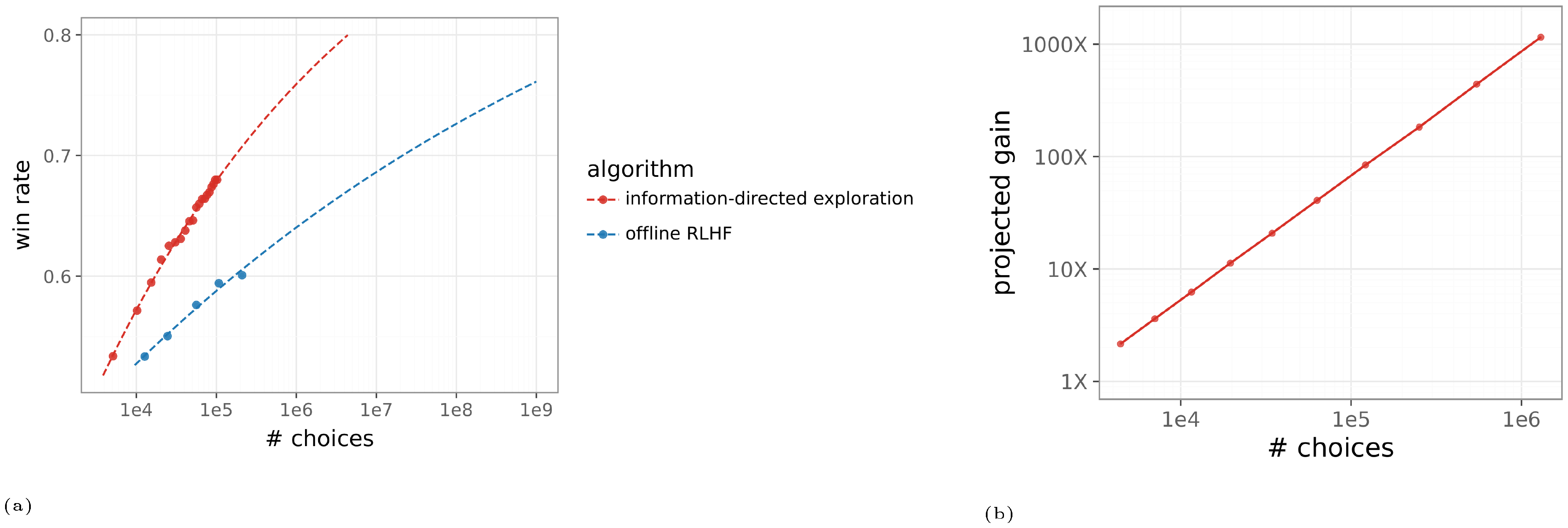
We develop an online learning algorithm that dramatically improves the data efficiency of reinforcement learning from human feedback (RLHF). Our algorithm incrementally updates reward and language models as choice data is received. The reward model is fit to the choice data, while the language model is updated by a variation of reinforce, with reinforcement signals provided by the reward model. Several features enable the efficiency gains: a small affirmative nudge added to each reinforcement signal, an epistemic neural network that models reward uncertainty, and information-directed exploration. With Gemma large language models (LLMs), our algorithm matches the performance of offline RLHF trained on 200K labels using fewer than 20K labels, representing more than a 10x gain in data efficiency. Extrapolating from our results, we expect our algorithm trained on 1M labels to match offline RLHF trained on 1B labels. This represents a 1,000x gain. To our knowledge, these are the first results to demonstrate that such large improvements are possible.

Correspondence: [email protected]

Executive Summary: The rapid advancement of large language models (LLMs) has made them powerful tools for tasks like writing, coding, and problem-solving, but aligning them with human preferences remains a major hurdle. Traditional methods require vast amounts of labeled data from humans comparing model responses, which is costly and time-consuming. As AI systems grow more capable, efficiently gathering this "right" data becomes crucial for building safe, helpful models that avoid unintended behaviors, especially in the pursuit of advanced AI that benefits society without risks.

This document develops and tests a new algorithm for reinforcement learning from human feedback (RLHF), a process that fine-tunes LLMs using human preferences. The goal is to show that an online approach—updating models incrementally as feedback arrives—can achieve the same performance as standard offline methods but with far less data.

The researchers compared four RLHF variants using a simulation of human choices based on the advanced Gemini 1.5 Pro model, which mimics complex real-world preferences better than smaller models. They drew from a diverse set of 202,000 unique prompts covering topics from math to creative writing, splitting them into 200,000 for training, 1,000 for tuning, and 1,000 for final evaluation. Responses were generated by a 9-billion-parameter Gemma LLM, with feedback simulated in batches of 64 prompts each. Key innovations in the leading algorithm included a small "affirmative nudge" to stabilize training, a neural network that estimates uncertainty in reward predictions, and a strategy to select response pairs most likely to yield informative feedback. Performance was measured by win rate: the average preference for the trained model over a baseline on out-of-sample prompts.

The core findings highlight dramatic efficiency gains. First, the new information-directed exploration algorithm matched the performance of offline RLHF—using 200,000 labels—after just under 20,000 labels, a more than 10-fold reduction in data needs. Second, it outperformed simpler online and periodic updates by avoiding performance drops common in those methods, thanks to the stabilizing nudge and uncertainty modeling. Third, gains grew with scale: extrapolating curves showed the algorithm could reach offline RLHF levels trained on 1 billion labels using only 1 million labels, projecting a 1,000-fold efficiency boost. Fourth, examples illustrated practical benefits, like generating concise, correct math solutions where offline methods produced convoluted errors, and selecting diverse responses that resolved key uncertainties, such as sentiment or comprehension differences.

These results mean organizations can align LLMs much faster and cheaper, slashing human labeling costs from millions to thousands of examples while improving response quality. This counters recent studies suggesting RLHF plateaus with more data, proving scalable methods can unlock better performance and safer AI deployment. By focusing on informative feedback, the approach reduces risks of misalignment, such as biased or unhelpful outputs, and shortens timelines for real-world applications like chatbots or educational tools.

Leaders should prioritize integrating information-directed exploration into RLHF pipelines, starting with pilot tests on internal datasets to confirm gains in actual use. If scaling to real human labelers, begin with smaller prompt sets and monitor for transfer from simulations. Further steps include validating results with live human feedback, refining uncertainty models for deeper integration, and extending to prompt selection or multiturn dialogues—potentially doubling efficiency again. Trade-offs: online methods demand more compute during training but pay off in data savings; without them, projects risk stalling on labeling bottlenecks.

While the simulation used a superior Gemini model to proxy human judgments, it may not capture all real-world nuances, like cultural biases or fatigue in labelers—real trials are needed for full confidence. Assumptions, such as fixed prompt diversity, held in this controlled setup, but edge cases like adversarial inputs could alter outcomes. Overall, confidence is high in the demonstrated 10x gains within this framework, but executives should approach 1,000x projections cautiously until validated at scale.

1. Introduction

Section Summary: Large language models have absorbed massive datasets, but a key future challenge is collecting the most useful data to build new abilities and align them with human values for safe superintelligent AI. This paper introduces an efficient reinforcement learning from human feedback algorithm that updates reward and language models step by step as people choose between response options, incorporating innovations like a subtle boost to learning signals, a network that tracks reward uncertainty, and targeted exploration to make the most of limited data. Experiments show it achieves over 10 times better data efficiency than standard methods after just 20,000 choices, with projections of up to 1,000 times as more data is used, marking a breakthrough for large models; the report then covers related work, methods, results, and future directions.

While today’s large models have learned from vast amounts of data, one critical challenge going forward is to gather the right data. Gathering more informative data can greatly accelerate learning not only of new capabilities but also of human preferences needed to guide how those capabilities are applied. Indeed, efficient exploration should serve as a cornerstone on the path to safe artificial superintelligence.

This paper develops an algorithm for reinforcement learning from human feedback (RLHF). Our algorithm incrementally updates reward and language models as human choices between alternative responses are observed. The reward model (RM) is fit to the choice data, while the language model (LM) is updated by a variation of reinforce, with reinforcement signals provided by the RM. Three notable innovations enable large gains in data efficiency: a small affirmative nudge added to each reinforcement signal, an epistemic neural network that models reward uncertainty, and information-directed exploration.

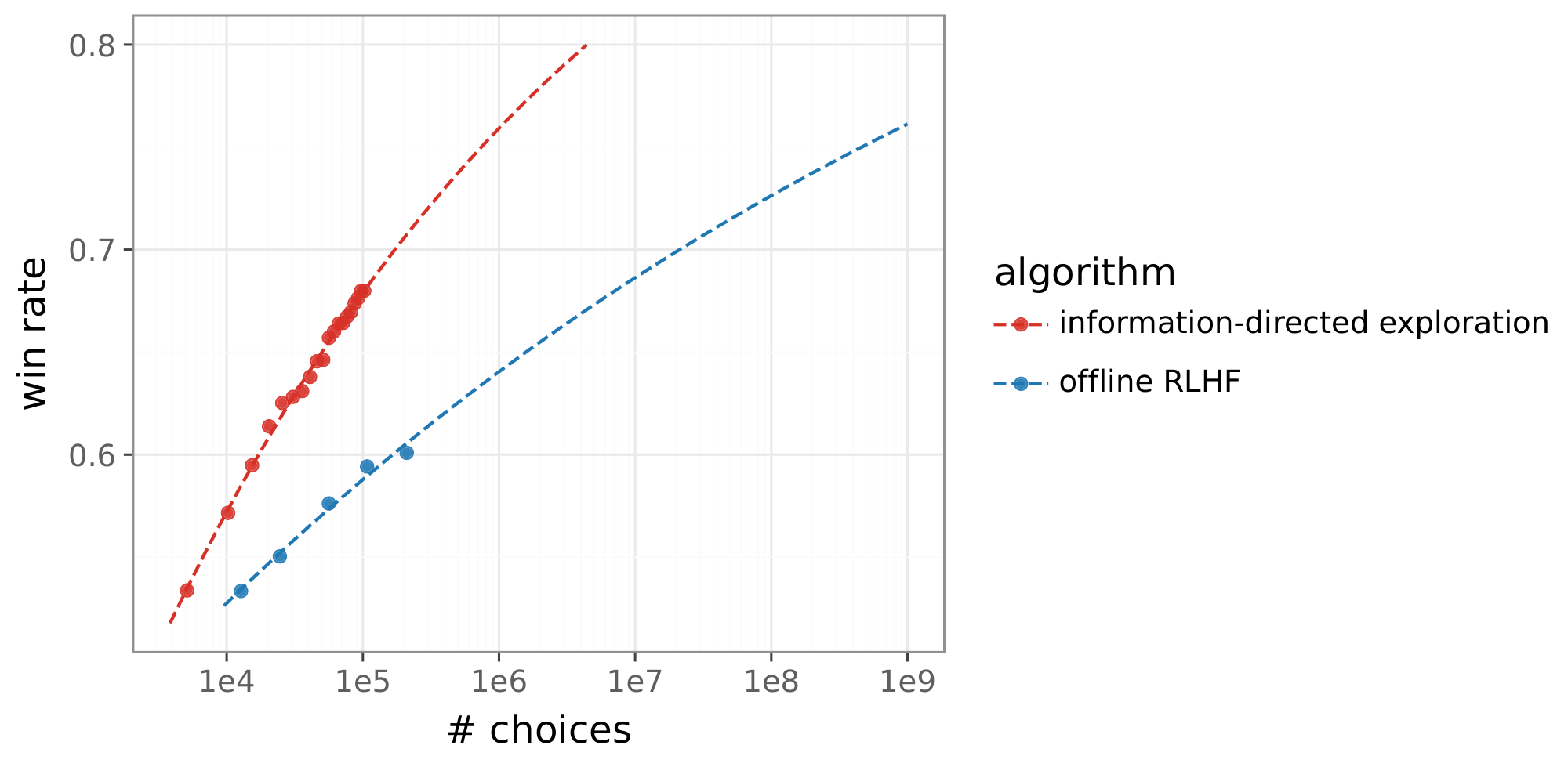
Figure 1 illustrates these data efficiency gains relative to an offline RLHF baseline. After observing fewer than 20K choices, our algorithm matches the performance of offline RLHF trained on 200K choices, representing more than a 10x gain in data efficiency. The gain is projected to grow with more choice data. With 1M choices, our algorithm is projected to reach a gain of 1, 000x. To the best of our knowledge, these are the first results to demonstrate that such large gains are possible with large language models (LLMs).

The remainder of this report details these findings. Section 2 discusses relevant literature. We describe our experiment pipeline in Section 3 and learning algorithms in Section 4. Section 5 presents our empirical results, which demonstrate the data efficiency gains. Finally, we conclude and discuss promising avenues for future work in Section 6.

2. Literature Review

Section Summary: This literature review examines how large language models can be efficiently aligned with human preferences using online adaptation techniques, which iteratively improve responses by sampling them in real-time rather than relying on fixed offline data. It also explores active exploration methods that select the most informative examples based on uncertainty or diversity to reduce the need for vast amounts of annotation, including approaches like preference optimization and exploration bonuses that guide sampling toward uncertain areas. Finally, the review discusses scaling laws showing that while models improve predictably with more data in early training stages, reinforcement learning from human feedback scales poorly with additional preference data, prompting a need for better techniques to uncover hidden patterns through logarithmic analysis.

Our work focuses on sample-efficient alignment of LLMs through active exploration and is related to work on online adaptation, active exploration, and scaling laws.

Online Adaptation. Work on online adaptation emphasizes iterative and sequential learning ([1, 2, 3]). Iterative versions of direct preference optimization (DPO), as investigated by [4], and hybrid preference optimization (HPO) ([5]) serve as examples. Recent studies demonstrate a clear advantage of online methods over their offline counterparts ([6]). This efficiency gain stems from the key difference that online algorithms sample responses on-policy, allowing them to constantly shift the response distribution toward better responses. Offline algorithms, which use a fixed sampling distribution, suffer from challenges related to data coverage and stationary learning targets.

Active Exploration. Traditional work on active exploration seeks to reduce annotation costs by selecting informative examples, often relying on uncertainty or diversity metrics ([7]). In LLM alignment, active exploration strategies that explicitly incorporate uncertainty and informativeness are central to improving sample efficiency. [8], [1], and [9] formalize this problem as an active contextual dueling bandit. [8] found that uncertainty-guided exploration can significantly improve reward models. However, their work focused exclusively on updating the RM, while the LM was fixed throughout the process. Techniques like active preference optimization (APO) and its variants, apply active learning principles directly to preference-based objectives (like DPO), iteratively collecting choice data that resolve uncertainty ([10, 9, 11]). Techniques like exploratory preference optimization (XPO) and those based on information-directed sampling (IDS) incorporate exploration bonuses to steer the policy toward sampling where the reward model's estimates are uncertain ([12, 13, 14]). Some other approaches harness the LLM itself to guide this exploration. Some methods utilize the model's output variability such as measuring the disagreement across multiple generated responses as a proxy for uncertainty ([15, 16]). The aforementioned literature reports gains of 2X to 5X and works with a much more limited range of prompts than our diverse set.

Scaling Laws. The scaling properties of large language models, which yield considerable performance improvements with more data, are key to their success. While these scaling laws have been studied extensively for both the pre-training stage ([17, 18]) and supervised fine-tuning ([19]), how reinforcement learning from human feedback (RLHF) improves with data is less understood. Recent studies have begun to explore related aspects, such as scaling laws for reward models ([20, 21, 22]). Nevertheless, a systematic understanding of how overall RLHF performance scales with the quantity of preference data remains elusive. This issue is compounded by the recent study suggesting that, disappointingly, current RLHF techniques demonstrate limited scalability, yielding only insignificant performance gains even when the quantity of preference data is substantially increased ([23]). This raises a critical question: can current RLHF techniques improve performance as more data becomes available or must we develop new techniques with better scaling properties? Our work is the first to systematically study the scaling laws governing performance as a function of the amount of human data. Papers proposing new RLHF algorithms often plot performance against the quantity of human data. However, plots with a linearly scaled horizontal axis obscure salient patterns. Using instead a logarithmic scale, as in Figure 1, reveals qualitative differences between scaling laws.

3. Experiment Pipeline

Section Summary: This section outlines an experiment pipeline for training and evaluating large language model policies, particularly to test reinforcement learning from human feedback algorithms, starting with a baseline policy from a 9-billion-parameter Gemma model that's deterministic and trained through initial pretraining and fine-tuning. To gather feedback, the pipeline uses a simulator based on a more advanced Gemini model to mimic human preferences by generating two diverse responses per prompt from a top-5 sampling method and selecting one via a probabilistic model, processing prompts in batches to update the policy iteratively. Performance is then assessed by comparing the updated policy against the baseline on a separate set of prompts, calculating a win rate based on how often the simulator prefers the new responses.

In this section, we present the experimentation pipeline used to train and compare LLM policies. We use this pipeline to assess the performance of RLHF algorithms.

3.1 Baseline and Experimentation Policies

To produce a baseline policy, we use a 9B Gemma model ([24]). Given approximately nine billion model parameters $\theta_0$, a prompt $X$, and a partial response $Y_1, \ldots, Y_{\ell-1}$, the model specifies a next token distribution $\pi_{\theta_0}(\cdot|X, Y_1, \ldots, Y_{\ell-1})$. The model can be used to sample a response $Y$ sequentially, token by token, until one indicates termination.

We interpret the manner in which $\pi_\theta$ samples each next token as a policy. But we consider a class of policies, which we refer to as top- $K$ policies. Given $X, Y_1, \ldots, Y_{\ell-1}$, the top- $K$ policy first identifies the set $\mathcal{Y}\ell$ of $K$ tokens $y \in \mathcal{Y}\ell$ that attain the largest probabilities $\pi_{\theta_0}(y|X, Y_1, \ldots, Y_{\ell-1})$ and then samples an element of $\mathcal{Y}\ell$ according to the corresponding conditional probabilities. If $K$ is equal to the number of tokens, the top- $K$ policy simply samples from the predictive distribution $\pi{\theta_0}(\cdot|X, Y_1, \ldots, Y_\ell)$.

As a baseline, we use the top- $1$ policy with parameters $\theta_0$, which result from pretraining and supervised fine-tuning (SFT) of the Gemma model, but not RLHF. This policy serves as a benchmark for comparison against improved top- $1$ policies based on different parameters. Note that the baseline policy is deterministic in the sense that $X, Y_1, \ldots, Y_\ell$ determine $Y_{\ell+1}$.

To sample candidate responses for experimentation when querying human feedback, will use top- $5$ policies with suitable parameters. Note that top- $5$ policies are typically stochastic. Use of such a policy diversifies responses so that a human choice between alternative responses is informative.

3.2 Human Feedback Simulator

We simulate human feedback using a reward model that is based on the Gemini 1.5 Pro LLM ([25]), trained on real human feedback. Given a prompt $X$ and two responses $(Y_1, Y_2)$, this simulator computes two reward values $(R_1, R_2)$ and maps these to a preference probability $P = \exp(R_1) / (\exp(R_1) + \exp(R_2))$ via the Bradley-Terry model ([26]) with an exponential score function. Then, a simulated human choice $C \sim \mathtt{Bernoulli}(P)$ is sampled.

It is worth noting that the Gemini Pro model is much larger than 9B Gemma models. As such, the simulated choices reflect behaviors far more complex than baseline or competing policies that we consider. We train and test policies on such complex choice behaviors so that our results are more likely to carry over to real human choices, which may also reflect behaviors more complex than LLMs.

3.3 Prompts

We use a set of 202K prompts sampled from an internal repository routinely used for post-training. These prompts cover a wide range of topics such as writing, coding, summarization, reading comprehension, math, science, ideation, etc. Each prompt is unique and the set is randomly ordered. Within our experiment pipeline, we use 200K prompts for training, 1K for testing and hyperparameter selection, and 1K for out-of-sample evaluation.

3.4 Gathering Feedback and Training

When gathering feedback for training, an algorithm iterates through the training prompts. For each prompt, the algorithm generates two responses and receives a choice from the human feedback simulator, as illustrated in Figure 2. Prompts are grouped into batches of 64. After generating responses and observing choices for each batch of 64, the algorithm can adjust parameters to improve its policy based on the feedback. We denote by $\theta_t$ the policy parameters obtained after gathering $t$ batches of choice data.

3.5 Performance Evaluation

Given policy parameters $\theta_t$, we compare performance against the baseline parameters $\theta_0$ by evaluating a win rate. This involves iterating over the 1K out-of-sample prompts. For each such prompt $X$, we generate responses $Y_1$ and $Y_2$ using top- $1$ policies with parameters $\theta_t$ and $\theta_0$, respectively. As illustrated in Figure 3, given the prompt $X$ and responses $(Y_1, Y_2)$, the human feedback simulator produces a preference probability $P$. The win rate $\overline{P}$ is an average of the preference probability over the 1K out-of-sample prompts. An outcome of $\overline{P} = 1$ implies that the competing model is always chosen over the baseline, while an outcome of $\overline{P} = 0$ implies the opposite. Intermediate values of $\overline{P}$ indicate decrease of preference for the competing model over the baseline.

4. Algorithms

Section Summary: This section outlines four algorithms for improving AI language models through reinforcement learning from human feedback: offline RLHF, which collects all data upfront before training; periodic RLHF, which periodically gathers and trains on data in chunks; online RLHF, which updates models incrementally with each new batch; and information-directed exploration, which adds uncertainty modeling to guide data collection. All algorithms share a base model from a pre-trained Gemma 9B language model, with reward models predicting preferences between response pairs and policies optimized using gradient-based updates that incorporate regularization to stay close to initial behaviors. The updates use standard techniques like AdamW optimization, and the section provides motivation and key details without full implementation instructions.

We will compare performance across four alternative algorithms. While we will later explain these alternatives in greater detail, the following brief descriptions differentiate each:

1. offline RLHF: Gather $T$ batches of choice data with responses generated using $\pi_{\theta_0}$, then fit a reward model (initialized with $\phi_0$), then optimize the policy (initialized with $\theta_0$) to produce $\theta_T$.
2. periodic RLHF: For some period $\tau$ that is a fraction of $T$, produce a sequence of policies $\theta_{k \tau}: k = 1, 2, \ldots, T/\tau$. For each $k$, gather $\tau$ batches with responses generated by $\pi_{\theta_{(k-1)\tau}}$, then fit a reward model (to $k\tau$ batches, initialized with $\phi_0$), then optimize the policy (initialized with $\theta_0$) to produce $\theta_{k\tau}$.
3. online RLHF: Generate a sequence of policies $\pi_{\theta_t}: t = 1, 2, 3, \ldots$. For each $t$, gather a batch with responses generated using $\pi_{\theta_{t-1}}$, then incrementally adjust the reward model, then incrementally adjust $\theta_{t-1}$ to produce $\theta_t$.
4. information-directed exploration: Apply online RLHF but incrementally adjust a model of reward uncertainty alongside the point estimate reward model and use that to guide response selection.

In each case, $\phi_0$ and $\theta_0$ denote initial parameters of the reward model and policy. These four alternatives were developed through trial and error, in each case iterating over algorithm designs and hyperparameters while adhering to the above descriptions. Reward models and policies across these alternatives use approximately the same number of parameters. Also, parameter update rules are similar across the alternatives. We will describe common elements across reward models, policies, and update rules, and then explain each alternative in greater detail. Our intention is not to provide sufficient detail to reproduce our results but to share salient elements of our algorithms along with some motivation.

4.1 Reward Models and Policies

The initial parameters $\theta_0$ result from pretraining and supervised fine-tuning (SFT) of a Gemma 9B model. Each reward model is initialized with the same transformer backbone – that is, the the same language model $\pi$ with the unembedding matrix and softmax removed. The output of the backbone, which we refer to as the last-layer embedding, is then mapped to a scalar reward via a head, initialized with random weights.

For offline RLHF, periodic RLHF, and online RLHF, we use a linear head. For information-directed sampling, we use an ensemble of multilayer perceptron (MLP) heads, as we will motivate and describe further later. Use of an MLP rather than linear head did not improve the performance of other algorithms.

We denote the initial reward model by $r_{\phi_0}$, where $\phi_0$ is the vector of parameters, including those of the backbone and the head. Each of our algorithms update parameters of reward model and policy.

4.2 Update Rules

We now discuss update rules that we use to adjust reward model and policy parameters. Given a prompt $X$ and two responses $Y$ and $Y'$ a reward model $r_{\phi_t}$ predicts the probability that $Y$ will be chosen over $Y'$:

$ p_{\phi_t}(Y \succeq Y'|X) = \frac{e^{r_{\phi_t}(Y|X)}}{e^{r_{\phi_t}(Y|X)} + e^{r_{\phi_t}(Y'|X)}}. $

Suppose a prompt and pair of responses is presented to a rater, and we denote the chosen response by $Y$ and the other by $Y'$. Then, our reward model update rule computes a gradient

$ \Delta \phi_t = \nabla_{\phi_t} \ln p_{\phi_t}(Y \succeq Y'| X).\tag{1} $

These gradients are summed over a batch of prompts. We will later explain how each of our algorithms selects a pair of responses for each prompt. The gradients are summed over a batch of prompts, clipped, and then used to update $\phi_t$ and obtain $\phi_{t+1}$ using AdamW ([27]).

The policy update rule is slightly more complex. It entails maintaining an exponential moving average of parameters

$ \overline{\theta}_{t+1} = \eta \overline{\theta}t + (1-\eta) \theta{t+1}, $

for some $\eta \in (0, 1)$. We refer to $\overline{\theta}_t$ as an anchor. Parameters $\theta_t$ are regularized toward this anchor as they are updated. Given a prompt $X$ and a pair $(Y, Y')$ of responses, our update rule computes a policy gradient

$ \Delta \theta_t = \left(p_{\overline{\phi}t}(Y \succeq Y' | X) - \frac{1}{2}\right) \nabla{\theta_t} \ln \pi_{\theta_t}(Y|X) - \beta \sum_{\ell=1}^{\mathrm{len}(Y)} \pi_{\overline{\theta}t}(Y\ell | X, Y_{1:\ell-1}) \nabla_{\theta_t} \ln \frac{\pi_{\overline{\theta}t}(Y\ell | X, Y_{1:\ell-1})}{\pi_{\theta_t}(Y_\ell | X, Y_{1:\ell-1})}.\tag{2} $

The parameter $\beta$ weights the degree of regularization toward the anchor. Note that $\overline{\phi}_t$ denotes reward function weights used to update $\theta_t$; our online algorithms use $\overline{\phi}t = \phi_t$, while other algorithms use different parameters. The update rule can be viewed as a variant of reinforce ([28]) with reinforcement signal $p{\phi_t}(Y \succeq Y' | X) - 1/2$ or, alternatively, as a variant of PMPO ([29]).

Policy gradients are summed over a batch of prompts and multiple response pairs assigned to each prompt. We will later explain how each of our algorithms selects these response pairs. Policy gradients are summed, clipped, and then used to update policy parameters using AdamW. The gradients are summed over a batch of prompts, clipped, and then used to update using AdamW ([27]). One or more such adjustments are made to generate the difference $\theta_{t+1} - \theta_t$ between gathering the $t$ th and $(t+1)$ th batches of choice data.

4.3 Alternatives

We now explain in greater detail key features of each alternative algorithm beyond the aforementioned common elements.

4.3.1 Offline RLHF

Recall that our offline RLHF algorithm gathers $T$ batches of choice data, with response pairs sampled independently using top- $5$ sampling with parameters $\theta_0$. For each $t$-th batch, the reward model update rule Equation (1) is applied to adjust parameters, taking them from $\phi_{t-1}$ to $\phi_t$.

In order to optimize the policy, we assign to each prompt two (ordered) response pairs: a random pair sampled by the top- $5$ policy with parameters $\theta_t$ and those two responses in reverse order. Given a batch of prompts with two response pairs assigned to each, the policy update rule Equation (2) with $\overline{\phi}t = \phi_T$ is applied, with all gradients summed and then clipped to adjust parameters, taking them from $\theta_t$ to $\theta{t+1}$. Every 160th parameter vector $\theta_0, \theta_{160}, \theta_{320}, \ldots, \theta_T$ is stored. The final policy parameters are taken to be the vector among these checkpoints that maximizes win-rate on the test set.

4.3.2 Periodic RLHF

Periodic RLHF operates much in the same way as offline RLHF. Given a period $\tau$ that is a fraction of $T$, periodic RLHF carries out offline RLHF over $\tau$ instead of $T$ batches. This produces policy parameters $\theta_\tau$. Then, an additional $\tau$ batches of choice data are gathered but using response pairs sampled by the top- $5$ policy with parameters $\theta_\tau$ instead of $\pi_{\theta_0}$, a reward `function initialized at $r_{\phi_0}$ and a policy initialized at $\pi_{\theta_0}$ are updated just as in offline RLHF but using the $2\tau$ batches of data gathered so far. This process repeats, gathering $\tau$ batches of data using each new vector of policy parameters until $T$ batches have been gathered and processed. In our experiments, we use a period of $\tau = 400$ batches.

Relative to offline RLHF, periodically updating the language model in this way is known to improve performance ([3]). The degree of improvement grows as the period $\tau$ shrinks. However, the number of times one trains new models also grows, and the approach becomes computationally onerous. Our online algorithm overcomes this obstacle by incrementally updating the RM and LM as choice data is observed, instead of training new models and policies from scratch.

4.3.3 Online RLHF

Our online RLHF algorithm interleaves between updates of reward model and policy parameters. While prior work ([30, 31, 32, 9]) has suggested promise in updating a policy directly, without a reward model, reward-model-free approaches we have tried have not proved to be competitive. Figure 4(left) plots the best performance we were able to obtain by updating a policy without a reward model. While showing some improvement over offline RLHF, the results are not competitive with our online RLHF algorithm, which does use a reward model.

:::: {cols="2"}

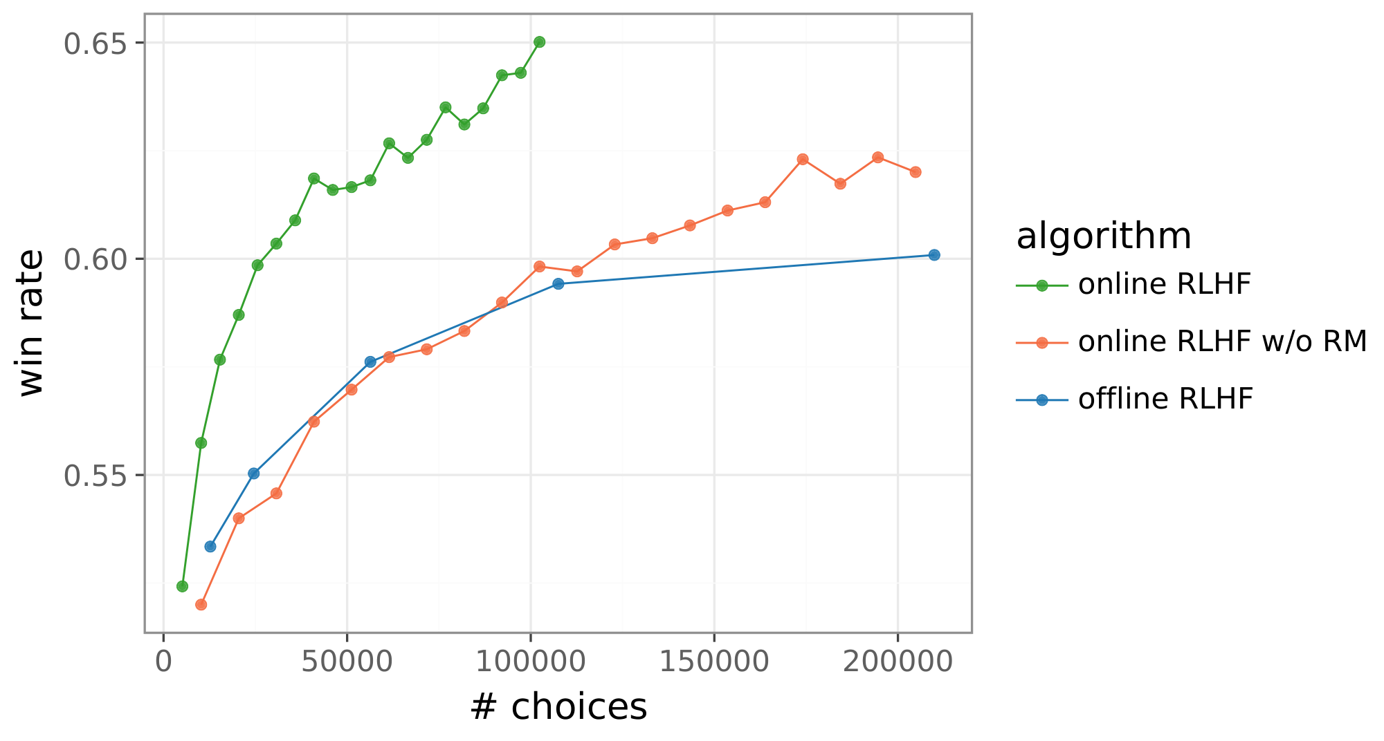
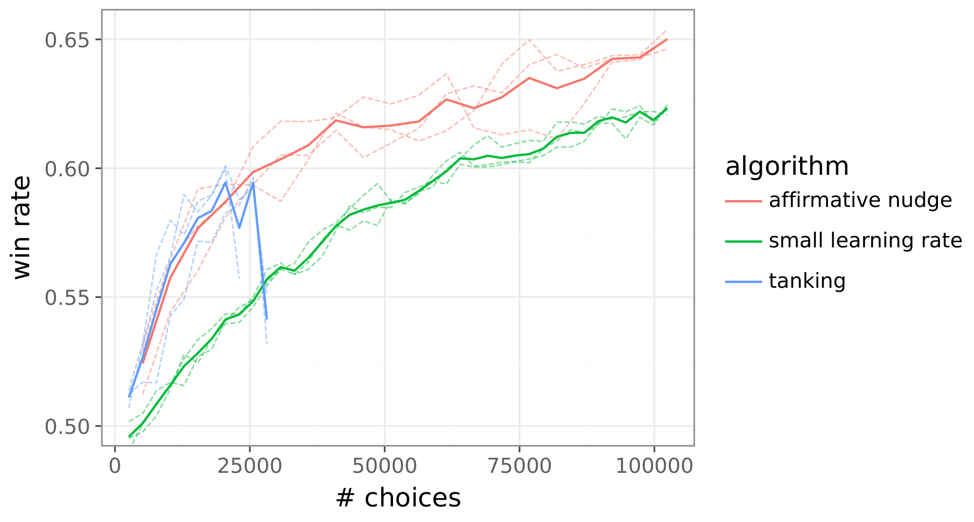
Figure 4: Strong performance of online RLHF relies on a reward function (left) and an affirmative nudge (right). ::::

Prior online RLHF algorithms tank after training on some number of batches, as illustrated in Figure 4(right). To address this, one can checkpoint previous policies and use one from before tanking or reduce the learning rate to delay tanking. As illustrated in the figure, each of these solutions sacrifices performance relative to our online RLHF algorithm. Via a slight modification of the policy update rule Equation (2), our algorithm avoids tanking without requiring a learning rate reduction. This is accomplished by adding a small positive scalar $\epsilon$, which we refer to as an affirmative nudge, to each reinforcement signal. The update rule becomes

$ \Delta \theta_t = \left(p_{\overline{\phi}t}(Y \succeq Y' | X) - \frac{1}{2} + \epsilon\right) \nabla{\theta_t} \ln \pi_{\theta_t}(Y|X) - \beta \sum_{\ell=1}^{\mathrm{len}(Y)} \pi_{\overline{\theta}t}(Y\ell | X, Y_{1:\ell-1}) \nabla_{\theta_t} \ln \frac{\pi_{\overline{\theta}t}(Y\ell | X, Y_{1:\ell-1})}{\pi_{\theta_t}(Y_\ell | X, Y_{1:\ell-1})}.\tag{3} $

Figure 4(right) demonstrates the benefit.

Our algorithm updates reward model parameters as follows. Given $\phi_t$ and $\theta_t$, for each prompt in a batch of 64, we sample sixteen responses using $\pi_{\theta_t}$ and query the human feedback simulator with a random selection of two among the sixteen. Given choices made by the simulator, the reward model update rule Equation (1) is applied to adjust parameters, taking them from $\phi_t$ to $\phi_{t+1}$.

To update policy parameters, we first compute gradients according to (3), with $\overline{\phi}t = \phi{t+1}$. For each of the aforementioned 64 prompts, we compute gradients for four pairs of responses. The first two are the response pair used in the query and the same pair in reverse order. The other two are selected from the sixteen samples based on reward estimates: (highest, lowest) and (lowest, highest). Note that rewards are assessed according to $r_{\phi_{t+1}}$. The gradients are summed and clipped and the result added to $\theta_t$. Then, for each of a new batch of 64 prompts, we sample 16 responses and select four pairs from among them based on reward estimates: (highest, lowest), (lowest, highest), (second-highest, second-lowest), and (second-lowest, second-highest). We again compute gradients according to (3) for each of these prompts with each of its four response pairs. Finally, these gradients are summed, clipped, and added to parameters to produce $\theta_{t+1}$.

4.3.4 Information-Directed Exploration

Our information-directed sampling algorithm relies on supplementing the reward model head with components that require a very small number of additional parameters relative to the overall number, which is around nine billion. These components enable uncertainty modeling. We use the uncertainty estimates to guide selection of responses when constructing queries for human feedback. The training is done in a manner similar to our online RLHF algorithm, except that we additionally train the new head components. We now offer further detail on the architecture, queries, and training.

Architecture

Our architecture includes a point estimate, which is identical to the architecture used by other algorithms except with the linear head replaced by an MLP with two hidden layers, each of width 1024, and a linear output node. We call this point estimate head $\mathtt{mlp 0}$. We supplement this head with an ensemble of MLPs, including 100 prior networks, each with two hidden layers of width 256, and 100 differential networks, each with two hidden layers of width 1024. We call the prior networks $\mathtt{\overline{mlp}\ 1}, \ldots, \mathtt{\overline{mlp}\ 100}$ and the differential networks $\mathtt{mlp\ 1}, \ldots, \mathtt{mlp\ 100}$. All of our MLPs are initialized with random weights. The prior and differential networks form an ensemble with randomized prior functions, as studied in ([33]).

:::: {cols="1"}

Figure 8: A neural network reward model versus an epistemic neural network reward model. ::::

Our architecture serves as an epistemic neural network (ENN), as studied in ([34]). While the reward model architecture used by previous algorithms takes as input a prompt $X$ and response $Y$ and outputs a reward $r_\phi(Y|X)$, as illustrated in Figure 8(left), the ENN reward model takes an additional input $Z$ and outputs a reward $r_\phi(Y|X, Z)$ that depends on $Z$. We denote choice probabilities by

$ p_{\phi_t}(Y \succeq Y'|X, Z) = \frac{e^{r_{\phi_t}(Y|X, Z)}}{e^{r_{\phi_t}(Y|X, Z)} + e^{r_{\phi_t}(Y'|X, Z)}}. $

$ \arg\max_{Y, Y'} \rm{Var}\left[p_{\psi}(Y \succeq Y'|X, Z)\right] $

We refer to $Z$ as an epistemic index. In our ENN reward model, $Z$ can take on integer values from $0$ to $100$. If $Z=0$, the model carries out inference via the point estimate reward model, as illustrated in Figure 12. On the other hand, if $Z > 0$ then values of the $Z$ th prior and differential networks are added, as illustrated in Figure 13.

While our ENN reward model requires an increase in the number of parameters, the increase is small relative to the nine billion parameters in the original model. In particular, the percentage increase is well under 5%.

Queries

Given policy and reward model parameters $\phi_t$ and $\theta_t$, for each prompt in a batch of 64, we sample sixteen responses using $\pi_{\theta_t}$. For each prompt $X$ and pair $(Y, Y')$ of responses, we compute the variance $p_{\phi_t}(Y \succeq Y'|X, Z)$ over ensemble particles $Z=1, \ldots, 100$. We then select the response pair $(Y_*, Y_*')$ that maximizes this variance and send the query $(X, Y_*, Y_*')$ to the human feedback simulator. The motivation is to select a response pair for which a choice will be informative, and the choice probability variance serves as a measure of informativeness.

Training

Given a batch of 64 queries and choices, we update the point estimate reward model in exactly the same way as done in our online RLHF algorithm. In particular, we use the same loss function but based on the output $r(Y|X, 0)$, and we leave the prior and differential networks untouched in this step. We then update each of the differential networks, individually, using the same loss function, with losses computed based on $r(Y|X, Z)$ for $Z=1, \ldots, 100$. When updated each of these differential networks, the backbone parameters are frozen. The prior networks are never updated in the training process.

5. Results

Section Summary: The results show that information-directed exploration significantly outperforms offline RLHF in win rates for adapting language models, achieving better performance with far less data—needing only 20,000 choices to match what offline RLHF requires over 200,000, a tenfold efficiency gain. Extrapolations predict even larger advantages, up to 1,000 times more efficient after a million choices. Examples illustrate this through simple math problems, where the efficient method delivers concise, correct answers unlike the convoluted errors from offline RLHF, and by selecting diverse response pairs to gather more informative feedback on preferences.

We now present and interpret results produced by applying each of the aforementioned algorithms in our experiment pipeline.

5.1 Win Rates

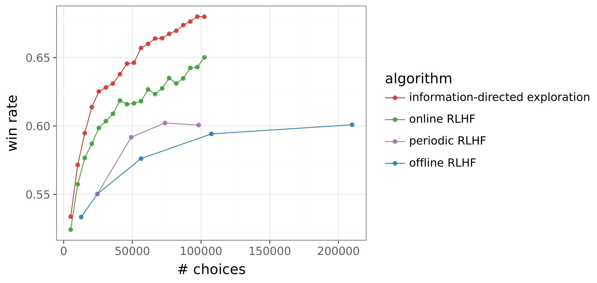
Figure 14 plots win rates attained by each of our algorithms as a function of the number of choices observed. While the win rate of offline RLHF improves with the number of choices, the alternatives do much better. Information-directed exploration, in particular, demonstrates large improvement. Offline RLHF needs more than 200K choices to match that performance at 20K choices. This represents an over 10x gain in data efficiency.

5.2 Projected Gains

To further interpret the implications of these gains, Figure 15a extrapolates win rates attained by information-directed exploration and offline RLHF, and Figure 15b maps these curves to projected data efficiency gains relative to offline RLHF. These gains increase with the number of choices, leading to a gain of about 1, 000x after a million choices are observed by the online algorithm.

5.3 Simple and Extreme Instances

Instances of prompts and responses foster intuition on what drives the data efficiency gains that we have demonstrated. In this section, we present some that are simple so that they are easy to digest and extreme so that they emphasize salient behavior.

5.4 Winning Responses

Our first example illustrates how a winning response generated by information-directed exploration improves over one generated by offline RLHF.

Consider the following simple prompt, which asks for the answer to a multiple choice math problem.

prompt:	If a person walks at 14 km/hr instead of 10 km/hr, he would have walked 20 km
	more. The actual distance traveled by him is:
	A. 50 km
	B. 56 km
	C. 70 km
	D. 80 km

A model produced by the offline RLHF method generates the response below, which is convoluted and arrives at a wrong answer.

offline RLHF:	Here's how to solve the problem:
	1. Understand the concept of time: The key is to realize that the
	time taken to cover a distance remains the same in both scenarios
	(walking at 10 km/hr and 14 km/hr).
	2. Set up variables:
	Let ' $d'$ be the actual distance traveled.
	Let ' $t'$ be the time taken to travel the distance.
	3. Formulate equations:
	We can express the distance in terms of speed and time for both
	scenarios:
	$d = 10t$ (distance at 10 km/hr)
	$d + 20 = 14t$ (distance at 14 km/hr, which is 20 km more)
	4. Solve for ' $d'$:
	Now we have two equations, and we can solve for ' $d'$. One way is
	through substitution:
	1. Solve the first equation for ' $t'$: $t = d/10$
	2. Substitute this value of ' $t'$ into the second equation:
	$d + 20 = 14(d/10)$
	3. Simplify and solve for ' $d'$: $d + 20 = (7/5)d$
	$(3/5)d = 20$
	$d = 100/3$ km
	Therefore, the actual distance traveled is approximately 33.33 km.
	None of the provided answer choices are correct.

A model produced by information-directed exploration, on the other hand, generates a more concise response and, importantly, coherent logic leading up to the correct answer.

efficient exploration:	Here's how to solve the problem:
	1. Time Difference: The person covers the extra 20 km because of
	the increased speed (14 km/hr - 10 km/hr = 4 km/hr). To cover
	20km at this extra speed, it takes him 20 km / 4 km/hr = 5 hours.
	2. Distance at Original Speed: Since he walked for 5 hours at his
	original speed of 10 km/hr, the actual distance traveled is
	5 hours * 10 km/hr = 50 km.
	Therefore, the answer is A.

5.5 Diverse Responses

Recall that our information-directed exploration algorithm selects responses to maximize the variance of choice probability based on an ENN reward model. We next present two examples that illustrate how this elicits informative feedback. For each prompt, we generated sixteen responses and select two response pairs: one that maximizes choice probability variance and one that minimizes choice probability variance. We refer to these as infomax and infomin response pairs.

Note that whether a pair is expected to elicit informative feedback changes as labels are collected and our uncertainty model is trained on that data. For example, if the uncertainty model infers from data collected thus far that one response is highly likely to be preferred over another then it will attribute little expected information gain to the pair. To produce the examples below, we used the initial ENN reward model parameters $\theta_0$.

Our first example prompts for sentiment expressed by a comment on water intake.

prompt:	Is this a negative or a positive sentiment? Do not provide reasons.
	Keep in mind that about 20% of our total water intake comes not from
	beverages but from water-rich foods like lettuce, leafy greens, cucumbers,
	bell peppers, summer squash, celery, berries, and melons.

Responses in the infomin pair express the same content.

infomin 1:	Positive.
infomin 2:	Positive sentiment.

Responses in the infomax pair carry differing meanings and therefore elicit an informative choice.

infomax 1:	positive
infomax 2:	Neutral.

Our second example entails an exercise in reading comprehension.

prompt:	According to the article below, what was the main reason for executive order
	6102?
	[begin article]
	The stated reason for the order was that hard times had caused a "hoarding"
	of gold, stalling economic growth and worsening the depression as the US was
	then using the gold standard for its currency.
	On April 6, 1933, The New York Times wrote, under the headline Hoarding of
	Gold, "The Executive Order issued by the President yesterday amplifies and
	particularizes his earlier warnings against hoarding. On March 6, taking
	advantage of a wartime statute that had not been repealed, he issued
	Presidential Proclamation 2039 that forbade the hoarding 'of gold or silver
	coin or bullion or currency', under penalty of $10, 000 fine or ten years
	imprisonment or both."
	The main rationale behind the order was actually to remove the constraint on
	the Federal Reserve preventing it from increasing the money supply during
	the depression. The Federal Reserve Act (1913) required 40% gold backing
	of Federal Reserve Notes that were issued. By the late 1920s, the Federal
	Reserve had almost reached the limit of allowable credit, in the form of
	Federal Reserve demand notes, which could be backed by the gold in its
	possession.
	[end article]

As with our first example, the infomin pair presents two responses that make equivalent statements.

infomin 1:	The article states that the main rationale behind Executive Order 6102
	was to remove the constraint on the Federal Reserve preventing it from
	increasing the money supply during the depression.
infomin 2:	The article states the main reason for executive order 6102 was to
	remove the constraint on the Federal Reserve preventing it from
	increasing the money supply during the depression.

The infomax pair, on the other hand, provides responses with substantially different forms of reasoning to support the conclusion.

infomax 1:	The main reason Executive Order 6102 was issued was to remove
	the constraint on the Federal Reserve preventing it from increasing
	the money supply to fight the Great Depression.
	Here's why:
	$\bullet$ The gold standard: The US was using the gold standard, meaning
	the value of the dollar was fixed to a certain amount of gold. This
	system limited the Fed's ability to create new money to stimulate
	the economy.
	$\bullet$ The Depression's impact: The Great Depression had severely
	restricted lending and economic activity. The Fed's limited ability
	to increase the money supply hindered efforts to boost the economy.
	$\bullet$ Executive Proclamation 2039: This order expanded upon President
	Roosevelt's earlier Proclamation 2039, which prohibited gold and
	silver hoarding. This further aimed to reduce the supply of gold,
	which could have helped the Fed increase the money supply.
infomax 2:	The main reason for Executive Order 6102, according to the
	provided article, was to remove the constraint on the Federal
	Reserve preventing it from increasing the money supply during the
	depression.
	The article states: "The main rationale behind the order was
	actually to remove the constraint on the Federal Reserve preventing
	it from increasing the money supply during the depression."
	The article also explains that the Federal Reserve Act of 1913
	required 40% gold backing for their notes, which they had almost
	reached by the late 1920s. This restriction prevented the Fed from
	creating more money to stimulate the economy. The order allowed
	the Fed to bypass this restriction and increase the money supply.

6. Conclusions and Future Work

Section Summary: The researchers showed that online learning and a method called uncertainty-guided exploration can greatly improve how efficiently AI models like large language models learn from human feedback, by avoiding common problems and focusing on the most informative responses, potentially making them 1,000 times more efficient than traditional approaches. They achieved this by training special networks to measure and maximize useful information from feedback. Looking ahead, they suggest further enhancements like better ways to handle uncertainty, selecting better prompts or conversations, extending to multi-turn dialogues and AI agents, and using AI to help humans provide more detailed feedback.

We have demonstrated that online learning and uncertainty-guided exploration each offer enormous gains in data efficiency. To realize the gains from online learning, we needed to overcome the tanking behavior commonly observed in the course of RLHF. We did this by introducing an affirmative nudge. Our specific approach uncertainty-guided exploration relied on training an epistemic neural network and selecting responses to maximize a measure of information gain.

While our algorithms point to a potential 1, 000x data efficiency gain relative to offline RLHF, we believe there remains much room for improvement through further research. Beyond improving algorithms, there is opportunity to translate benefits to other large language model use cases. Some promising research directions that could build on this work include:

• improving the exploration algorithm. There are a number of ways to improve our algorithm that warrant further research. Among them are modeling uncertainty deeper in reward models, representing uncertainty not just about the reward model but also the language model, and developing more efficient optimization algorithms that train the language model using information from the reward model.
• selecting prompts. While the exploration algorithm we presented is designed to select responses given a prompt, it can be extended to select prompts that are expected to yield informative feedback.
• multiturn dialog. Our pipeline and methods can be extended to optimize the quality of multiturn conversations. One approach, introduced by [35], involves learning not only a reward model but also a value model that predicts anticipated rewards. Our approach can be extended to work with such value models.
• agents. Our methods could also be extended to optimizing the performance of AI agents. Again, ideas from ([35]) may be helpful to learning from human feedback when actions induce delayed consequences. Our approach can be extended to this work to produce better agents.
• AI assisted feedback. As AI capabilities advance and responses become more complex, comparison of responses becomes too challenging for humans. A promising direction is AI-assisted feedback, where the AI actively frames the comparison to elicit more informative feedback. For instance, a human could validate an AI-generated rationale for why one response is superior to another. The debate paradigm of [36] offers an example. Our methods could be applied to this richer feedback structure to further enhance its informativeness.

Acknowledgments

Section Summary: The acknowledgments section expresses gratitude for helpful discussions with numerous colleagues from DeepMind and later Google DeepMind that enriched the research. Among those thanked are Ian Osband, Geoffrey Irving, Rich Sutton, Shi Dong, Junhyuk Oh, Zeyu Zheng, Rishabh Joshi, David Silver, Satinder Baveja, Doina Precup, Yee Whye Teh, Jasper Snoek, James Harrison, Bo Dai, Kevin Murphy, and Shibl Mourad. These conversations provided valuable insights and inspiration for the work.

This work benefited from stimulating conversations with many colleagues at DeepMind and then Google Deepmind, including Ian Osband, Geoffrey Irving, Rich Sutton, Shi Dong, Junhyuk Oh, Zeyu Zheng, Rishabh Joshi, David Silver, Satinder Baveja, Doina Precup, Yee Whye Teh, Jasper Snoek, James Harrison, Bo Dai, Kevin Murphy, and Shibl Mourad.

References

Section Summary: This references section lists over 30 academic papers, preprints, and books primarily focused on advancing large language models in artificial intelligence, with a strong emphasis on techniques like reinforcement learning from human feedback (RLHF) to make AI more helpful and aligned with user preferences. It includes works on efficient sampling and exploration methods to reduce the data needed for training, scaling laws that explain how model performance improves with more resources, and foundational studies in active learning and neural networks. Several entries cover practical applications, such as open models like Gemma and Gemini, alongside theoretical insights into optimization and safety in AI development.

[1] Viraj Mehta et al. (2025). Sample Efficient Preference Alignment in LLMs via Active Exploration. In Second Conference on Language Modeling.

[2] Hanze Dong et al. (2024). RLHF Workflow: From Reward Modeling to Online RLHF. Transactions on Machine Learning Research.

[3] Bai et al. (2022). Training a helpful and harmless assistant with reinforcement learning from human feedback. arXiv preprint arXiv:2204.05862.

[4] Xiong et al. (2024). Iterative Preference Learning from Human Feedback: Bridging Theory and Practice for RLHF under KL-constraint. In Proceedings of the 41st International Conference on Machine Learning. pp. 54715–54754.

[5] Avinandan Bose et al. (2025). Hybrid Preference Optimization for Alignment: Provably Faster Convergence Rates by Combining Offline Preferences with Online Exploration. In ICLR Workshop: Quantify Uncertainty and Hallucination in Foundation Models: The Next Frontier in Reliable AI.

[6] Tang et al. (2024). Understanding the performance gap between online and offline alignment algorithms. arXiv preprint arXiv:2405.08448.

[7] Settles, Burr (2009). Active learning literature survey.

[8] Dwaracherla et al. (2024). Efficient Exploration for LLMs. In Proceedings of the 41st International Conference on Machine Learning. pp. 12215–12227. https://proceedings.mlr.press/v235/dwaracherla24a.html.

[9] Kaixuan Ji et al. (2025). Reinforcement Learning from Human Feedback with Active Queries. Transactions on Machine Learning Research.

[10] Das et al. (2025). Active preference optimization for sample efficient RLHF. In Joint European Conference on Machine Learning and Knowledge Discovery in Databases. pp. 96–112.

[11] Muldrew et al. (2024). Active Preference Learning for Large Language Models. In Proceedings of the 41st International Conference on Machine Learning. pp. 36577–36590.

[12] Tengyang Xie et al. (2025). Exploratory Preference Optimization: Harnessing Implicit $Q^$-Approximation for Sample-Efficient RLHF*. In The Thirteenth International Conference on Learning Representations.

[13] Qi et al. (2025). Sample-Efficient Reinforcement Learning From Human Feedback via Information-Directed Sampling. IEEE Transactions on Information Theory. 71(10). pp. 7942-7958.

[14] Liu et al. (2024). Sample-efficient alignment for LLMs. arXiv preprint arXiv:2411.01493.

[15] Diao et al. (2024). Active prompting with chain-of-thought for large language models. In Proceedings of the 62nd Annual Meeting of the Association for Computational Linguistics (Volume 1: Long Papers). pp. 1330–1350.

[16] Bayer et al. (2026). ActiveLLM: Large Language Model-Based Active Learning for Textual Few-Shot Scenarios. Transactions of the Association for Computational Linguistics. 14. pp. 1-22. doi:10.1162/TACL.a.63. https://doi.org/10.1162/TACL.a.63.

[17] Kaplan et al. (2020). Scaling laws for neural language models. arXiv preprint arXiv:2001.08361.

[18] Hoffmann et al. (2022). Training compute-optimal large language models. In Proceedings of the 36th International Conference on Neural Information Processing Systems.

[19] Zheng Yuan et al. (2023). Scaling Relationship on Learning Mathematical Reasoning with Large Language Models. arXiv:2308.01825.

[20] Leo Gao et al. (2022). Scaling Laws for Reward Model Overoptimization. arXiv:2210.10760.

[21] Rafailov et al. (2025). Scaling laws for reward model overoptimization in direct alignment algorithms. In Proceedings of the 38th International Conference on Neural Information Processing Systems.

[22] Karl Cobbe et al. (2021). Training Verifiers to Solve Math Word Problems. arXiv:2110.14168.

[23] Zhenyu Hou et al. (2024). Does RLHF Scale? Exploring the Impacts From Data, Model, and Method. arXiv:2412.06000.

[24] Gemma Team et al. (2024). Gemma 2: Improving Open Language Models at a Practical Size. https://arxiv.org/abs/2408.00118. arXiv:2408.00118.

[25] Gemini Team (2024). Gemini 1.5: Unlocking multimodal understanding across millions of tokens of context. https://arxiv.org/abs/2403.05530. arXiv:2403.05530.

[26] Ralph Allan Bradley and Milton E. Terry (1952). Rank Analysis of Incomplete Block Designs: I. The Method of Paired Comparisons. Biometrika. 39(3/4). pp. 324–345.

[27] Ilya Loshchilov and Frank Hutter (2017). Fixing Weight Decay Regularization in Adam. CoRR. abs/1711.05101.

[28] Sutton, Richard S. and Barto, Andrew G. (2018). Reinforcement Learning: An Introduction. MIT Press.

[29] Abbas Abdolmaleki et al. (2025). Learning from negative feedback, or positive feedback or both. In The Thirteenth International Conference on Learning Representations. https://openreview.net/forum?id=4FVGowGzQb.

[30] Shangmin Guo et al. (2024). Direct Language Model Alignment from Online AI Feedback. arXiv:2402.04792.

[31] Xiaoqiang Lin et al. (2026). ActiveDPO: Active Direct Preference Optimization for Sample-Efficient Alignment. In The Fourteenth International Conference on Learning Representations. https://openreview.net/forum?id=RD4XgyVyGh.

[32] Syrine Belakaria et al. (2025). Sharpe Ratio-Guided Active Learning for Preference Optimization in RLHF. In Second Conference on Language Modeling. https://openreview.net/forum?id=a6xzTqMUFQ.

[33] Osband et al. (2018). Randomized Prior Functions for Deep Reinforcement Learning.

[34] Ian Osband et al. (2023). Epistemic Neural Networks. In Thirty-seventh Conference on Neural Information Processing Systems.

[35] Marklund, Henrik and Van Roy, Benjamin (2024). Choice Between Partial Trajectories: Disentangling Goals from Beliefs. arXiv preprint arXiv:2410.22690.

[36] Irving et al. (2018). AI safety via debate. arXiv preprint arXiv:1805.00899.