Synthetic Data for Text Localisation in Natural Images

Ankush GuptaAndrea VedaldiAndrew Zisserman

article2016CVPR1,575 citations

Presents a scalable engine for generating geometrically aligned synthetic text in natural scenes, proving that deep detectors trained purely on synthetic data can achieve state-of-the-art, real-time text localization.

Listen

Detecting and reading text in natural images is a critical capability for modern computer vision applications, yet traditional systems remain slow, complex, and prone to error. While deep learning methods have achieved near-perfect accuracy when reading pre-cropped words, the initial step of locating text in cluttered environments has remained a major operational bottleneck. A primary obstacle to training high-performing neural networks for this task has been the severe scarcity of large-scale, annotated real-world datasets, which are expensive and time-consuming to produce manually.

The article demonstrates that high-performance text detection models can be trained entirely on automatically generated synthetic data without any manual annotation. Its primary objective is to introduce a realistic synthetic image generation engine alongside an efficient, fully-convolutional deep learning architecture for rapid and accurate text localization in natural scenes.

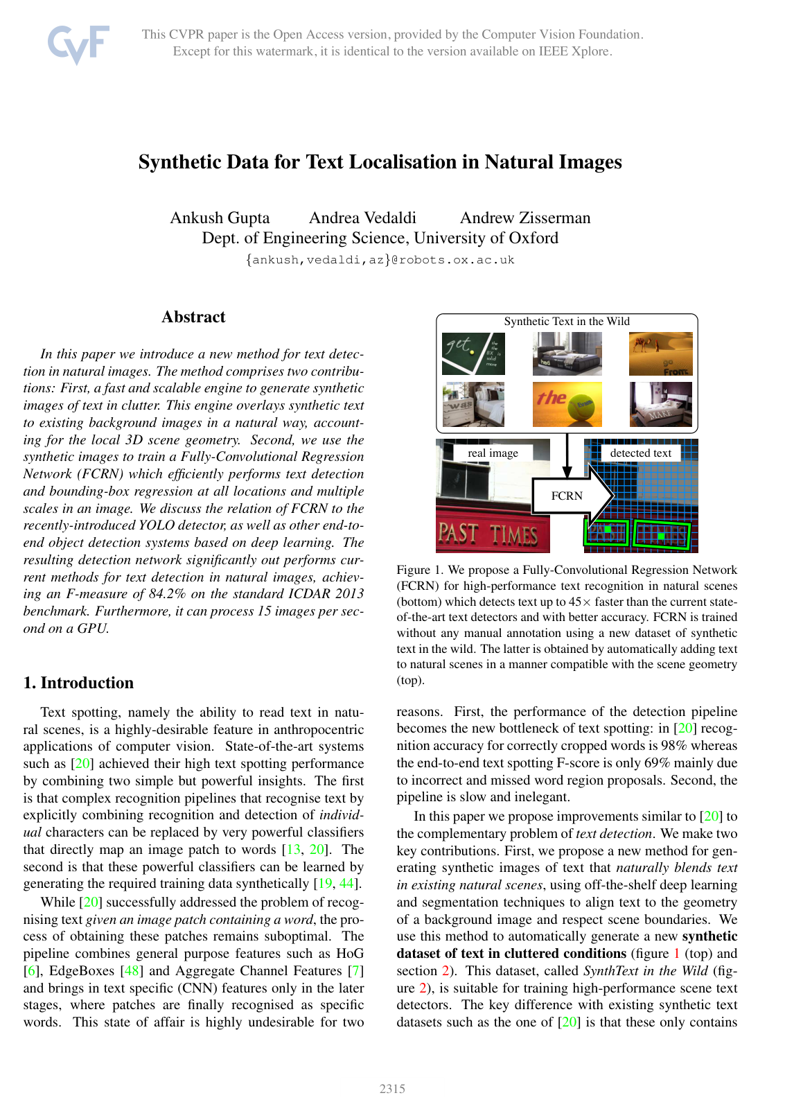
To achieve this, the authors developed an automated synthetic engine that takes clean background images, estimates local depth and surface boundaries, and naturally blends rendered text into the scenes according to local 3D geometry and realistic color profiles. This pipeline generated 800,000 synthetic training images containing multiple annotated words. Using exclusively this synthetic dataset, the authors trained a compact Fully-Convolutional Regression Network that predicts text presence and precise bounding-box coordinates directly across dense image locations and multiple scales, eliminating the need for slow multi-stage region proposal pipelines.

The findings show substantial improvements in both detection accuracy and processing speed. When evaluated on standard benchmarks such as ICDAR 2013, the proposed model achieved a state-of-the-art F-measure of 84.2%, outperforming previous methods by approximately 8 percentage points. On challenging datasets like Street View Text, the model delivered notable recall and average precision gains. In ablation tests, aligning synthetic text to local scene geometry and color boundaries proved vital, yielding significantly better real-world performance than training on randomly pasted text. Operationally, the model processed up to 15 images per second on a single GPU—running the initial text proposal stage roughly 45 times faster than standard approaches and speeding up end-to-end reading pipelines by a factor of 3 to 23.

These results demonstrate that high-quality synthetic data can effectively eliminate data collection bottlenecks and reduce development costs for computer vision systems. By streamlining the detection architecture into an efficient single-pass network, the approach makes real-time text recognition practical on hardware-constrained deployments without sacrificing accuracy. Furthermore, retraining existing older architectures on the large synthetic dataset produced only minimal gains, confirming that architectural design and realistic data synthesis must work in tandem.

Organizations developing computer vision pipelines should adopt synthetic generation techniques that respect scene geometry to train detection models, replacing multi-stage proposal frameworks with unified convolutional regressors. For production deployments, teams should weigh the trade-off between speed and recall: using high-confidence detections provides ultra-fast processing (about 0.3 seconds per image), whereas processing all candidate proposals provides maximum detection accuracy at a slightly higher computational cost.

Key limitations include difficulty detecting text in highly unusual fonts, missing very small text due to the lack of image upscaling, and occasional false detections caused by non-text patterns with uniform stroke widths, such as stick figures or road signs. The reported performance on unannotated datasets like Street View Text may also underestimate actual precision due to incomplete benchmark labeling. Overall confidence in the findings is high, as the synthetic-only training approach consistently outperformed existing baselines across multiple independent benchmarks.

Cover for Synthetic Data for Text Localisation in Natural Images

Abstract

In this paper we introduce a new method for text detection in natural images. The method comprises two contributions: First, a fast and scalable engine to generate synthetic images of text in clutter. This engine overlays synthetic text to existing background images in a natural way, accounting for the local 3D scene geometry. Second, we use the synthetic images to train a Fully-Convolutional Regression Network (FCRN) which efficiently performs text detection and bounding-box regression at all locations and multiple scales in an image. We discuss the relation of FCRN to the recently-introduced YOLO detector, as well as other end-to-end object detection systems based on deep learning. The resulting detection network significantly out performs current methods for text detection in natural images, achieving an F-measure of 84.2% on the standard ICDAR 2013 benchmark. Furthermore, it can process 15 images per second on a GPU.

Table of Contents

  • 1 Introduction
  • 1.1 Related Work
  • 2 Synthetic Text in the Wild
  • 2.1 Text and Image Sources
  • 2.2 Segmentation and Geometry Estimation
  • 2.3 Text Rendering and Image Composition
  • 3 A Fast Text Detection Network
  • 3.1 Architecture
  • 4 Evaluation
  • 4.1 Datasets
  • 4.2 Text Localisation Experiments
  • 4.3 Synthetic Dataset Evaluation
  • 4.4 End-to-End Text Spotting
  • 4.5 Timings
  • 5 Conclusion
  • References
  • A Appendix
  • A.1 Variation in Fonts, Colors and Sizes
  • A.2 Poisson Editing vs. Alpha Blending
  • A.3 SynthText in the Wild
  • A.4 ICDAR 2013 Detections
  • A.5 Street View Text (SVT) Detections

Knowls

  1. Knowl 1 — SynthText in the Wild Synthetic Scene-Text Generation Pipeline

    algorithm

    The SynthText in the Wild generation pipeline automatically synthesizes realistic annotated text in natural scene images by respecting local surface geometry and color/texture boundaries at an average generation speed of approximately 0.5 seconds per image.

    Input: Background image IRGBI_{RGB}, Text corpus TT, Cropped word dataset Dcolor\mathcal{D}_{color}, Font set F\mathcal{F}
    Output: Synthetic scene-text image IsynI_{syn} with character- and word-level ground truth bounding boxes
    1. Sample text string S∼TS \sim T at word, line (up to 3 lines), or paragraph (up to 7 lines) level.
    2. Obtain dense pixel-wise depth map DD for IRGBI_{RGB} using a single-image depth CNN.
    3. Compute contour hierarchies on IRGBI_{RGB} using gPb-UCM and threshold at 0.11 to obtain contiguous candidate regions R\mathcal{R}.
    4. For each region R∈RR \in \mathcal{R}:
         a. Discard RR if its area is too small, its aspect ratio is extreme, its normal is orthogonal to the viewing ray, or its texture score (norm of 3rd RGB derivatives) exceeds a threshold.
         b. Fit a 3D planar facet to depth DD over region RR using RANSAC to estimate local surface normal nR\mathbf{n}_R.
    5. For each retained region RR:
         a. Warp region contour of RR to a fronto-parallel view using normal nR\mathbf{n}_R.
         b. Fit a bounding rectangle to the fronto-parallel region; align the text layout along the rectangle's longer axis (width).
         c. Check for spatial collision with previously placed text masks in RR.
         d. Partition pixels of word crops in Dcolor\mathcal{D}_{color} into two clusters via K-means to form foreground-background color pairs.
         e. Find the color pair minimizing the L2L_2 distance in Lab color space to the mean color of RR; assign the foreground color to text SS.
         f. With probability 0.20, add an outline border whose color is a value-shifted foreground color or the mean of foreground and background colors.
         g. Render text SS using a randomly selected font from F\mathcal{F}, apply the 3D perspective homography corresponding to normal nR\mathbf{n}_R, and blend rendered text into IRGBI_{RGB} using Poisson image editing.
    6. return IsynI_{syn} and the corresponding tight bounding box annotations.
  2. Knowl 2 — Fully-Convolutional Regression Network Architecture for Text Detection

    model/method

    The Fully-Convolutional Regression Network (FCRN) performs dense text presence classification and bounding-box regression across an image via fully convolutional operations.

    The feature extraction backbone consists of nine convolutional layers with Rectified Linear Unit (ReLU) activations and four max-pooling layers, structured in the following sequential order:

    1. Convolution: 64 filters of size 5×55 \times 5 (CR-64-5x5), followed by 2×22 \times 2 Max-Pooling with stride 2 (MP).
    2. Convolution: 128 filters of size 5×55 \times 5 (CR-128-5x5), followed by MP.
    3. Convolutions: two layers of 128 filters of size 3×33 \times 3 (CR-128-3x3, CR-128-3x3), followed by MP.
    4. Convolutions: two layers of 256 filters of size 3×33 \times 3 (CR-256-3x3, CR-256-3x3), followed by MP.
    5. Convolutions: two layers of 512 filters of size 3×33 \times 3 (CR-512-3x3, CR-512-3x3), followed by one convolution of 512 filters of size 5×55 \times 5 (CR-512-5x5).

    All convolutional filters operate with stride 1 and use zero-padding to preserve feature map resolution. The four downsampling max-pooling layers produce a cumulative spatial stride of Δ=16\Delta = 16 pixels, yielding a 512-channel dense feature map.

    On top of this backbone, a prediction head consisting of seven linear convolutional filters of size 5×55 \times 5 (C-7-5x5) outputs 7 values per grid cell. For an input image of size H×WH \times W, the network outputs a spatial prediction tensor of dimensions HΔ×WΔ×7\frac{H}{\Delta} \times \frac{W}{\Delta} \times 7 (e.g., 14×14×714 \times 14 \times 7 for a 224×224224 \times 224 input). The complete network requires 44 MB of memory.

  3. Knowl 3 — FCRN Bounding Box Parameterization and Objective Function

    equation

    For an image of size H×WH \times W processed with feature stride Δ=16\Delta = 16, each predictor centered at pixel grid cell coordinates (u,v)(u, v) predicts a text presence confidence c∈Rc \in \mathbb{R} and a 6-dimensional normalized geometric pose vector pˉ\bar{p}:

    pˉ=(x−uΔ,  y−vΔ,  wW,  hH,  cos⁡θ,  sin⁡θ)\bar{p} = \left(\frac{x - u}{\Delta},\; \frac{y - v}{\Delta},\; \frac{w}{W},\; \frac{h}{H},\; \cos \theta,\; \sin \theta\right)

    where (x,y)(x, y) denotes the center coordinates of the ground-truth word bounding box in pixels, (w,h)(w, h) are the box width and height, and θ\theta is the bounding box rotation angle. A predictor at cell (u,v)(u, v) is responsible for detecting a word if the word center (x,y)(x, y) lies within the cell region of size Δ×Δ\Delta \times \Delta.

    The training loss is the sum of squared errors across all HΔ×WΔ×7\frac{H}{\Delta} \times \frac{W}{\Delta} \times 7 output elements. For grid cells that do not contain a ground-truth word center, the loss ignores all 6 pose parameters in pˉ\bar{p} and evaluates only the confidence score cc.

    To address severe class imbalance (only 1–2% of cells contain text), non-text confidence error terms are scaled by a factor λbg\lambda_{\text{bg}}, initialized at λbg=0.01\lambda_{\text{bg}} = 0.01 and gradually increased to λbg=1.0\lambda_{\text{bg}} = 1.0 over the course of training with Stochastic Gradient Descent.

  4. Knowl 4 — Multi-Scale Detection and Multi-Filtering Text Proposal Refinement Pipeline

    model/method

    Because the fixed receptive field of FCRN limits detection of large text instances, images are evaluated over a multi-scale pyramid with downscaling factors {1,1/2,1/4,1/8}\{1, 1/2, 1/4, 1/8\}. Detections across scales are merged via non-maximum suppression (NMS), where overlapping detections with lower confidence are suppressed.

    Two modes of FCRN proposals are evaluated:

    • Low-recall mode (FCRN + multi-filt): Retains only detections with confidence probability t>0.3t > 0.3, producing fewer than 30 proposals per image.
    • High-recall mode (FCRNall + multi-filt): Retains all multi-scale detections by setting threshold t=0.0t = 0.0, generating approximately 1000 candidate proposals per image.

    The candidate proposals are refined through a three-stage post-processing pipeline:

    1. Random Forest Filtering: A binary random forest classifier filters out non-text proposals.
    2. CNN Bounding-Box Regression: A convolutional neural network refines the bounding box coordinates.
    3. Word Recognition NMS: Text is recognized using a large-lexicon CNN classifier, and overlapping proposals predicting the same word identity are merged via non-maximum suppression.
  5. Knowl 5 — Text Localisation Benchmark Performance Across Datasets and Protocols

    data/table

    The table below compares the Fully-Convolutional Regression Network (FCRN) against baseline and prior text localization methods on ICDAR 2011 (IC11), ICDAR 2013 (IC13), and Street View Text (SVT) datasets under both PASCAL (IoU ≥0.5\ge 0.5) and DetEval evaluation protocols. FF is F-measure, PP is Precision, RR is Recall at maximum F-measure, and RMR_M is maximum achievable recall.

    PASCAL Eval DetEval
    IC11 IC13 SVT IC11 IC13 SVT
    Method FF PP RR RMR_M FF PP RR RMR_M FF PP RR RMR_M FF PP RR FF PP RR FF PP RR
    Huang - - - - - - - - - - - - 78 88 71 - - - - - -
    Jaderberg 77.2 87.5 69.2 70.6 76.2 86.7 68.0 69.3 53.6 62.8 46.8 55.4 76.8 88.2 68.0 76.8 88.5 67.8 24.7 27.7 22.3
    Jaderberg (SynthText) 77.3 89.2 68.4 72.3 76.7 88.9 67.5 71.4 53.6 58.9 49.1 56.1 75.5 87.5 66.4 75.5 87.9 66.3 24.7 27.8 22.3
    Neumann (2012) - - - - - - - - - - - - 68.7 73.1 64.7 - - - - - -
    Neumann (2013) - - - - - - - - - - - - 72.3 79.3 66.4 - - - - - -
    Zhang - - - - - - - - - - - - 80 84 76 80 88 74 - - -
    FCRN single-scale 60.6 78.8 49.2 49.2 61.0 77.7 48.9 48.9 45.6 50.9 41.2 41.2 64.5 81.9 53.2 64.3 81.3 53.1 31.4 34.5 28.9
    FCRN multi-scale 70.0 78.4 63.2 64.6 69.5 78.1 62.6 67.0 46.2 47.0 45.4 53.0 73.0 77.9 68.9 73.4 80.3 67.7 34.5 29.9 40.7
    FCRN + multi-filt 78.7 95.3 67.0 67.5 78.0 94.8 66.3 66.7 56.3 61.5 51.9 54.1 78.0 94.5 66.4 78.0 94.8 66.3 25.5 26.8 24.3
    FCRNall + multi-filt 84.7 94.3 76.9 79.6 84.2 93.8 76.4 79.6 62.4 65.1 59.9 75.0 82.3 91.5 74.8 83.0 92.0 75.5 26.7 26.2 27.4

    The FCRNall + multi-filt model achieves an F-measure of 84.2% on IC13 (PASCAL) and 83.0% (DetEval), outperforming previous state-of-the-art methods by approximately 6% to 8% in F-measure across benchmarks.

  6. Knowl 6 — Ablation of Synthetic Data Realism on Scene-Text Localization

    empirical result

    The contribution of geometric alignment and region-sensitive text placement in synthetic training data was evaluated by training the FCRNall + multi-filt model on three synthetic training datasets with identical text lexicons, background images, and color distributions, but increasing realism:

    1. Random Placement: Text rendered at random positions and orientations in background images without considering scene content.
      • SVT Performance: Maximum F-measure F=60.3%F = 60.3\%, Average Precision AP=50.6%\text{AP} = 50.6\%, Maximum Recall Rmax⁡=68.2%R_{\max} = 68.2\%.
    2. Colour/Texture Region Constraints: Text constrained within homogeneous color and texture regions derived from gPb-UCM segmentation.
      • SVT Performance: F=61.9%F = 61.9\% (+1.6%+1.6\% over random), AP=53.7%\text{AP} = 53.7\% (+3.1%+3.1\% over random), Rmax⁡=75.0%R_{\max} = 75.0\% (+6.8%+6.8\% over random).
    3. Perspective Distortion + Regions: Text constrained within segmented regions and perspectively warped according to local 3D surface normals estimated from dense depth maps.
      • SVT Performance: F=62.4%F = 62.4\% (+0.55%+0.55\% over regions alone), AP=54.5%\text{AP} = 54.5\% (+0.75%+0.75\% over regions alone), Rmax⁡=75.0%R_{\max} = 75.0\%.

    Constraining text to semantically and geometrically consistent regions provides the dominant performance gain, especially in maximum recall (+6.8%+6.8\%).

  7. Knowl 7 — End-to-End Text Spotting Benchmark Results

    data/table

    The table below compares end-to-end text spotting performance (detection combined with recognition using the lexicon-encoding CNN of Jaderberg et al.) in maximum F-measure percentage. Words shorter than 3 characters or with non-alphanumeric characters are excluded by standard protocol. Values in parentheses represent performance when non-alphanumeric words are retained.

    Model IC11 IC11* IC13 SVT SVT-50
    Wang et al. (2011) - - - - 38
    Wang Wu (2012) - - - - 46
    Alsharif Pineau (2013) - - - - 48
    Neumann Matas (2013) - 45.2 - - -
    Jaderberg et al. (2014) - - - - 56
    Jaderberg et al. (2015) 76 69 76 53 76
    FCRN + multi-filt 80.5 (77.8) 75.8 (73.5) 80.3 (77.8) 54.7 68.0
    FCRNall + multi-filt 84.3 (81.2) 81.0 (78.4) 84.7 (81.8) 55.7 67.7

    FCRNall + multi-filt improves end-to-end text spotting F-measure by over 8% on ICDAR 2011 and ICDAR 2013, and by 2.7% on SVT over the previous state-of-the-art.

  8. Knowl 8 — Inference Latency and Proposal Generation Speedup

    empirical result

    On an NVIDIA GPU with 512×512512 \times 512 pixel input images, FCRN achieves:

    • Single-scale inference throughput: 20 images per second (0.05 seconds per image).
    • Multi-scale inference throughput: 15 images per second (0.07 seconds per image) across four scale levels {1,1/2,1/4,1/8}\{1, 1/2, 1/4, 1/8\}.

    When replacing the region proposal stage in multi-stage text spotting pipelines, FCRN reduces proposal generation time from 3.00 seconds to 0.07 seconds per image, achieving a 43×43\times speedup in proposal generation.

    Total end-to-end spotting execution time per image:

    • FCRN + multi-filt (<30<30 proposals): 0.30 seconds total (0.07s proposal, 0.03s proposal filtering, 0.20s bounding box regression and recognition).
    • FCRNall + multi-filt (∼1000\sim 1000 proposals): 2.47 seconds total (0.07s proposal, 1.20s proposal filtering, 1.20s bounding box regression and recognition).
    • Jaderberg et al. baseline: 7.00 seconds total (3.00s proposal, 3.00s proposal filtering, 1.00s bounding box regression and recognition).

    FCRN + multi-filt is 23×23\times faster than the prior state-of-the-art end-to-end text spotting pipeline while achieving superior accuracy.

  9. Knowl 9 — FCRN Text Detector Limitations and Failure Modes

    limitation

    The FCRN detection pipeline exhibits four primary failure modes:

    1. Unseen Typography: Performance degrades on unusual or artistic fonts absent from the synthetic training font collection.
    2. False Positives on Text-like Structures: Non-text patterns with uniform stroke width and high local contrast (e.g., road signs, stick figures, abstract geometric symbols) can trigger false detections.
    3. Extremely Small Text: Because the multi-scale inference pyramid applies only downscaling factors (≤1.0\le 1.0) and avoids image upscaling, very low-resolution or distant text is missed.
    4. Word Fragmentation and Merging: Words with unusually large intra-character spacing are frequently split into multiple bounding boxes, whereas words with unusually tight inter-word spacing are frequently merged into a single detection.

Coverage note — None was omitted; all key contributions—the synthetic data generation engine, the FCRN architecture and loss formulation, multi-scale post-processing pipelines, benchmark evaluation data, dataset ablation, timing benchmarks, and failure modes—are covered.

References

  1. 1.O. Alsharif and J. Pineau. End-to-end text recognition with hybrid HMM maxout models. ArXiv e-prints, Oct 2013.
  2. 2.P. Arbelaez, M. Maire, C. Fowlkes, and J. Malik. Contour detection and hierarchical image segmentation. IEEE PAMI, 33:898–916, 2011.
  3. 3.P. Arbelaez, J. Pont-Tuset, J. Barron, F. Marques, and J. Malik. Multiscale combinatorial grouping. In Proc. CVPR, 2014.
  4. 4.D. J. Butler, J. Wulff, G. B. Stanley, and M. J. Black. A naturalistic open source movie for optical flow evaluation. In Proc. ECCV, 2014.
  5. 5.A. Criminisi, I. D. Reid, and A. Zisserman. Single view metrology. In Proc. ICCV, pages 434–442, 1999.
  6. 6.N. Dalal and B. Triggs. Histogram of Oriented Gradients for Human Detection. In Proc. CVPR, volume 2, pages 886–893, 2005.
  7. 7.P. Dollar, R. Appel, and S. Belongie. Fast feature pyramids for object detection. IEEE PAMI, 36(8):1532–1545, 2014.
  8. 8.A. Dosovitskiy and T. Brox. Inverting visual representations with convolutional networks. In Proc. CVPR, 2016. To appear.
  9. 9.A. Dosovitskiy, P. Fischer, E. Ilg, P. Hausser, C. Hazirbas, V. Golkov, P. Smagt, D. Cremers, and T. Brox. Flownet: Learning optical flow with convolutional networks. In Proc. ICCV, 2015.
  10. 10.M. A. Fischler and R. C. Bolles. Random sample consensus: A paradigm for model fitting with applications to image analysis and automated cartography. Comm. ACM, 24(6):381–395, 1981.
  11. 11.R. B. Girshick. Fast R-CNN. In Proc. ICCV, 2015.
  12. 12.R. B. Girshick, J. Donahue, T. Darrell, and J. Malik. Rich feature hierarchies for accurate object detection and semantic segmentation. In Proc. CVPR, 2014.
  13. 13.I. J. Goodfellow, Y. Bulatov, J. Ibarz, S. Arnoud, and V. Shet. Multi-digit number recognition from street view imagery using deep convolutional neural networks. In Proc. ICLR, 2014.
  14. 14.D. Hoiem, A. A. Efros, and M. Hebert. Automatic photo pop-up. In Proc. ACM SIGGRAPH, 2005.
  15. 15.D. Hoiem, A. A. Efros, and M. Hebert. Geometric context from a single image. In Proc. ICCV, 2005.
  16. 16.P. V. C. Hough. Method and means for recognizing complex patterns. US Patent 3,069,654, 1962.
  17. 17.W. Huang, Y. Qiao, and X. Tang. Robust scene text detection with convolution neural network induced mser trees. In Proc. ECCV, 2014.
  18. 18.S. Ioffe and C. Szegedy. Batch normalization: Accelerating deep network training by reducing internal covariate shift. In Proc. ICML, 2015.
  19. 19.M. Jaderberg, K. Simonyan, A. Vedaldi, and A. Zisserman. Synthetic data and artificial neural networks for natural scene text recognition. In Workshop on Deep Learning, NIPS, 2014.
  20. 20.M. Jaderberg, K. Simonyan, A. Vedaldi, and A. Zisserman. Reading text in the wild with convolutional neural networks. IJCV, 2015.
  21. 21.M. Jaderberg, A. Vedaldi, and A. Zisserman. Deep features for text spotting. In Proc. ECCV, 2014.
  22. 22.A. Janoch, S. Karayev, Y. Jia, J. T. Barron, M. Fritz, K. Saenko, and T. Darrell. A category-level 3-d object dataset: Putting the kinect to work. In ICCV Workshop on Consumer Depth Cameras in Computer Vision, 2011.
  23. 23.D. Karatzas, L. Gomez-Bigorda, A. Nicolaou, S. Ghosh, A. Bagdanov, M. Iwamura, J. Matas, L. Neumann, V. R. Chandrasekhar, S. Lu, et al. ICDAR 2015 robust reading competition. In Proc. ICDAR, pages 1156–1160, 2015.
  24. 24.D. Karatzas, F. Shafait, S. Uchida, M. Iwamura, S. R. Mestre, J. Mas, D. F. Mota, J. A. Almazan, L. P. de las Heras, et al. ICDAR 2013 robust reading competition. In Proc. ICDAR, pages 1484–1493, 2013.
  25. 25.K. Karsch, V. Hedau, D. Forsyth, and D. Hoiem. Rendering synthetic objects into legacy photographs. ACM Transactions on Graphics, 30(6):157, 2011.
  26. 26.A. Krizhevsky, I. Sutskever, and G. E. Hinton. ImageNet classification with deep convolutional neural networks. In NIPS, pages 1106–1114, 2012.
  27. 27.K. Lang and T. Mitchell. Newsgroup 20 dataset, 1999.
  28. 28.B. Leibe, A. Leonardis, and B. Schiele. Combined object categorization and segmentation with an implicit shape model. In Workshop on Statistical Learning in Computer Vision, ECCV, May 2004.
  29. 29.K. Lenc and A. Vedaldi. R-CNN minus R. In Proc. BMVC., 2015.
  30. 30.F. Liu, C. Shen, and G. Lin. Deep convolutional neural fields for depth estimation from a single image. In Proc. CVPR, 2015.
  31. 31.J. Long, E. Shelhamer, and T. Darrell. Fully convolutional networks for semantic segmentation. In Proc. CVPR, 2015.
  32. 32.A. Mishra, K. Alahari, and C. Jawahar. Scene text recognition using higher order language priors. Proc. BMVC., 2012.
  33. 33.L. Neumann and J. Matas. Real-time scene text localization and recognition. In Proc. CVPR, volume 3, pages 1187–1190, 2012.
  34. 34.L. Neumann and J. Matas. Scene text localization and recognition with oriented stroke detection. In Proc. ICCV, pages 97–104, December 2013.
  35. 35.P. Perez, M. Gangnet, and A. Blake. Poisson image editing. ACM Transactions on Graphics, 22(3):313–318, 2003.
  36. 36.J. Redmon, S. K. Divvala, R. B. Girshick, and A. Farhadi. You only look once: Unified, real-time object detection. In Proc. CVPR, 2016. To appear.
  37. 37.S. Ren, K. He, R. Girshick, and J. Sun. Faster R-CNN: Towards real-time object detection with region proposal networks. In NIPS, 2016.
  38. 38.A. Saxena, M. Sun, and A. Y. Ng. Make3d: Learning 3d scene structure from a single still image. IEEE PAMI, 31(5):824–840, 2009.
  39. 39.A. Shahab, F. Shafait, and A. Dengel. ICDAR 2011 robust reading competition challenge 2: Reading text in scene images. In Proc. ICDAR, pages 1491–1496, 2011.
  40. 40.N. Silberman, D. Hoiem, P. Kohli, and R. Fergus. Indoor segmentation and support inference from rgbd images. In Proc. ECCV, 2012.
  41. 41.K. Simonyan and A. Zisserman. Very deep convolutional networks for large-scale image recognition. In International Conference on Learning Representations, 2015.
  42. 42.K. Wang, B. Babenko, and S. Belongie. End-to-end scene text recognition. In Proc. ICCV, pages 1457–1464, 2011.
  43. 43.K. Wang and S. Belongie. Word spotting in the wild. In Proc. ECCV, 2010.
  44. 44.T. Wang, D. J. Wu, A. Coates, and A. Y. Ng. End-to-end text recognition with convolutional neural networks. In Proc. ICPR, pages 3304–3308, 2012.
  45. 45.C. Wolf and J. M. Jolion. Object count/area graphs for the evaluation of object detection and segmentation algorithms. International Journal on Document Analysis and Recognition, 8(4):280–296, 2006.
  46. 46.I. Yildirim, T. D. Kulkarni, W. A. Freiwald, and J. B. Tenenbaum. Efficient and robust analysis-by-synthesis in vision: A computational framework, behavioral tests, and modeling neuronal representations. In Annual Conference of the Cognitive Science Society, 2015.
  47. 47.Z. Zhang, W. Shen, C. Yao, and X. Bai. Symmetry-based text line detection in natural scenes. In Proc. CVPR, 2015.
  48. 48.C. L. Zitnick and P. Dollar. Edge boxes: Locating object proposals from edges. In Proc. ECCV, pages 391–405, 2014.

Citation

MLA
Gupta, A., et al. “Synthetic Data for Text Localisation in Natural Images”. arXiv, 2016, http://arxiv.org/abs/1604.06646v1.
APA
Gupta, A., Vedaldi, A., & Zisserman, A. (2016). Synthetic Data for Text Localisation in Natural Images. arXiv. http://arxiv.org/abs/1604.06646v1
Chicago
Gupta, A., A. Vedaldi, and A. Zisserman. 2016. “Synthetic Data for Text Localisation in Natural Images”. arXiv. http://arxiv.org/abs/1604.06646v1.
Harvard
Gupta, A., Vedaldi, A. and Zisserman, A. (2016) “Synthetic Data for Text Localisation in Natural Images”, arXiv [Preprint]. Available at: http://arxiv.org/abs/1604.06646v1.
Vancouver
1. Gupta A, Vedaldi A, Zisserman A (2016) Synthetic Data for Text Localisation in Natural Images. arXiv

BibTeX

@article{gupta2016synthetic,
  title = {Synthetic Data for Text Localisation in Natural Images},
  author = {Gupta, Ankush and Vedaldi, Andrea and Zisserman, Andrew},
  year = {2016},
  journal = {arXiv},
  url = {http://arxiv.org/abs/1604.06646v1},
  eprint = {1604.06646}
}
Metadata:arXiv

Source Code

This paper has an official code repository available. Click below to access the source code.

View Repository

Access the Paper

This paper is available from its original source. Click below to access the PDF.

Open PDF
License: IEEE