Rademacher and Gaussian Complexities: Risk Bounds and Structural Results

P. BartlettS. Mendelson

article2002JMLR3,331 citations

Establishes data-dependent generalization bounds using Rademacher and Gaussian complexities alongside structural composition rules that yield practical error guarantees for neural networks, kernel methods, and decision trees.

Listen

The paper develops data-dependent measures of function-class complexity, specifically Rademacher and Gaussian complexities, to derive tighter risk bounds for learning algorithms and to relate the complexity of composite classes to that of simpler basis classes. Traditional bounds that rely on fixed penalties such as VC-dimension often fail to adapt to the training sample and therefore produce overly conservative model-selection rules. The authors address this limitation by proving general error bounds expressed directly in terms of empirical Rademacher or Gaussian averages and by establishing structural inequalities that allow these averages to be computed or bounded for practical model families.

The central results establish that, with high probability, the true risk of any function is at most its empirical risk plus a term proportional to the Rademacher complexity of a suitably transformed class, plus a small additive deviation of order 1/√n. The same bounds hold when the Rademacher term is replaced by its Gaussian counterpart, which differs from it by at most a logarithmic factor. Additional lemmas show that these complexities are comparable to the maximum discrepancy of the class and that they satisfy natural monotonicity, scaling, and Lipschitz-composition properties. For classes formed by convex combinations, Boolean operations, or Lipschitz maps of simpler classes, the complexity of the composite is controlled by the sum of the complexities of the components, scaled by constants that depend only on the Lipschitz constants or the number of summands.

These abstract bounds translate into concrete improvements for concrete models. For decision trees the resulting penalty can be substantially smaller than a uniform VC-style term whenever many leaves receive little empirical mass. For two-layer neural networks with ℓ1 weight constraints the Gaussian complexity scales with the square root of the maximum pairwise distance among input coordinates, again data-dependent. For kernel expansions the same machinery yields a margin-based bound whose complexity term is proportional to the trace of the empirical kernel matrix. In each case the derived penalty decreases at rate 1/√n or faster and never exceeds the order of classical combinatorial-dimension bounds.

Because the penalties adapt to the observed sample, they support more reliable complexity-regularization procedures for model selection. The structural results further reduce the computational burden by allowing the optimization that defines the complexity to be performed only over the simpler basis classes rather than over the full composite class. The main limitation is that exact evaluation still requires solving a non-convex optimization problem whose difficulty grows with model size; practical use therefore depends on efficient approximation schemes or on further tightening of the structural inequalities.

Australian National University decision trees decision-theoretic gaussians Rademacher Complexity Gaussian Complexity VC-dimension

Bartlett et al (2002).pdf

Paper: A training algorithm for optimal margin classifiers, B. Boser et al. (1992). Reading the foundational optimal margin classifier paper provides the essential structural background on support vector machines and margin maximization that the source paper analyzes via Rademacher complexities.

Paper: Manifold Regularization: A Geometric Framework for Learning from Labeled and Unlabeled Examples, Mikhail Belkin et al. (2006). This paper extends the empirical complexity framework of the source into a manifold regularization setting to exploit geometric structures in both labeled and unlabeled data.

Cover for Rademacher and Gaussian Complexities: Risk Bounds and Structural Results

Abstract

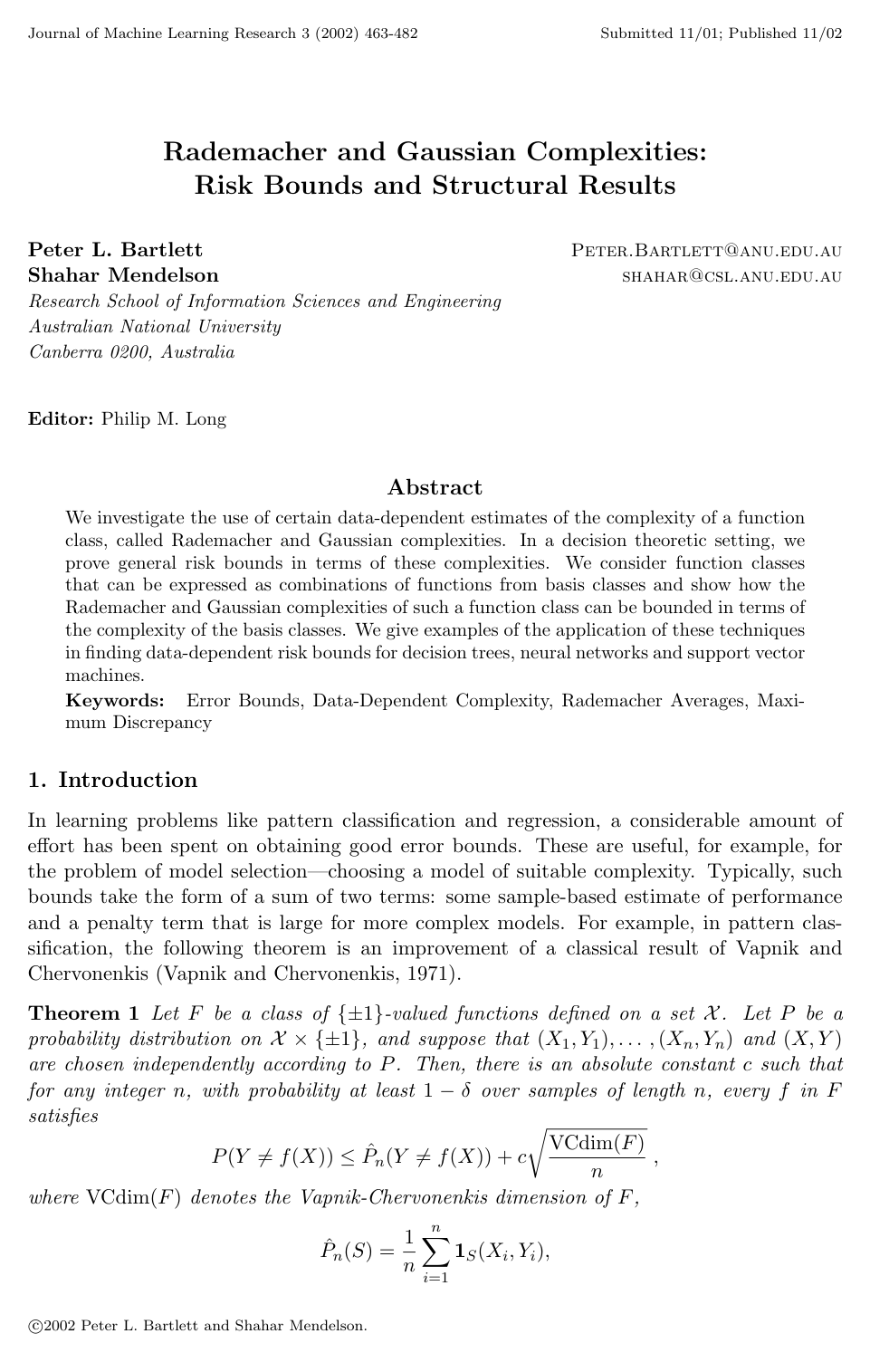
We investigate the use of certain data-dependent estimates of the complexity of a function class, called Rademacher and Gaussian complexities. In a decision theoretic setting, we prove general risk bounds in terms of these complexities. We consider function classes that can be expressed as combinations of functions from basis classes and show how the Rademacher and Gaussian complexities of such a function class can be bounded in terms of the complexity of the basis classes. We give examples of the application of these techniques in finding data-dependent risk bounds for decision trees, neural networks and support vector machines.

Topics

decision trees decision-theoretic gaussians neural networks support vector

Keywords

Rademacher Complexity Gaussian Complexity VC-dimension Maximum Discrepancy Risk Bound Structural Result Decision Tree Neural Network Support Vector Machine Margin

1. Introduction
2. Risk Bounds
3. Estimating the Rademacher and Gaussian Complexities of Function Classes
3.1 Simple Structural Results
3.2 Lipschitz Functions on $\mathbb{R}^k$
3.3 Boolean Combinations of Functions
4. Examples
4.1 Decision Trees
4.2 Neural Networks
4.3 Kernel Methods
Acknowledgments
Appendix A. Proof of Lemma 3
Appendix B. Proof of Theorem 5
References

Knowls

Knowl 1 — General Decision-Theoretic Risk Bound via Rademacher Complexity
theoretical result
Let $\mathcal{X}$ be an input space, $\mathcal{Y}$ an output space, and $\mathcal{A}$ an action space. Let $P$ be a probability measure on $\mathcal{X} \times \mathcal{Y}$ , and let $(X_1, Y_1), \dots, (X_n, Y_n)$ be an independent sample drawn according to $P$ . Let $\mathcal{L}: \mathcal{Y} \times \mathcal{A} \to [0, 1]$ be a loss function, and let $\phi: \mathcal{Y} \times \mathcal{A} \to [0, 1]$ be a dominating cost function satisfying $\phi(y, a) \ge \mathcal{L}(y, a)$ for all $y \in \mathcal{Y}$ and $a \in \mathcal{A}$ .

For a class $F$ of functions mapping from $\mathcal{X}$ to $\mathcal{A}$ , define the centered composite function class $\tilde{\phi} \circ F = \{(x, y) \mapsto \phi(y, f(x)) - \phi(y, 0) : f \in F\}.$

The expected Rademacher complexity $R_n(\tilde{\phi} \circ F)$ is defined as $R_n(\tilde{\phi} \circ F) = \mathbb{E}\left[ \sup_{f \in F} \left| \frac{2}{n} \sum_{i=1}^n \sigma_i \big(\phi(Y_i, f(X_i)) - \phi(Y_i, 0)\big) \right| \right],$ where $\sigma_1, \dots, \sigma_n$ are independent Rademacher random variables uniformly distributed on $\{\pm 1\}$ .

Then, for any integer $n \ge 1$ and any confidence parameter $\delta \in (0, 1)$ , with probability at least $1 - \delta$ over samples of length $n$ , every $f \in F$ satisfies $\mathbb{E}[\mathcal{L}(Y, f(X))] \le \frac{1}{n} \sum_{i=1}^n \phi(Y_i, f(X_i)) + R_n(\tilde{\phi} \circ F) + \sqrt{\frac{8 \ln(2/\delta)}{n}}.$
Knowl 2 — Rademacher Complexity, Gaussian Complexity, and Maximum Discrepancy
definition
Let $\mu$ be a probability distribution on a domain $\mathcal{X}$ , and let $X_1, \dots, X_n$ be independent samples drawn according to $\mu$ . Let $F$ be a class of real-valued functions mapping from $\mathcal{X}$ to $\mathbb{R}$ .
1. Maximum Discrepancy: The empirical maximum discrepancy is the random variable $\hat{D}_n(F) = \sup_{f \in F} \left( \frac{2}{n} \sum_{i=1}^{n/2} f(X_i) - \frac{2}{n} \sum_{i=n/2+1}^n f(X_i) \right),$ and the expected maximum discrepancy is $D_n(F) = \mathbb{E}[\hat{D}_n(F)]$ .
2. Rademacher Complexity: Let $\sigma_1, \dots, \sigma_n$ be independent uniform $\{\pm 1\}$ -valued random variables. The empirical Rademacher complexity conditioned on the sample is $\hat{R}_n(F) = \mathbb{E}_\sigma \left[ \sup_{f \in F} \left| \frac{2}{n} \sum_{i=1}^n \sigma_i f(X_i) \right| \;\middle|\; X_1, \dots, X_n \right],$ and the expected Rademacher complexity is $R_n(F) = \mathbb{E}[\hat{R}_n(F)]$ .
3. Gaussian Complexity: Let $g_1, \dots, g_n$ be independent standard Gaussian $\mathcal{N}(0, 1)$ random variables. The empirical Gaussian complexity conditioned on the sample is $\hat{G}_n(F) = \mathbb{E}_g \left[ \sup_{f \in F} \left| \frac{2}{n} \sum_{i=1}^n g_i f(X_i) \right| \;\middle|\; X_1, \dots, X_n \right],$ and the expected Gaussian complexity is $G_n(F) = \mathbb{E}[\hat{G}_n(F)].$ $
Knowl 3 — Structural Calculus Properties of Rademacher Complexity
theoretical result
Let $F, F_1, \dots, F_k$ , and $H$ be classes of real-valued functions mapping from a domain $\mathcal{X}$ to $\mathbb{R}$ . The expected Rademacher complexity $R_n$ satisfies the following structural properties:
1. Monotonicity: If $F \subseteq H$ , then $R_n(F) \le R_n(H)$ .
2. Convex and Absolute Convex Hulls: $R_n(F) = R_n(\mathrm{conv}(F)) = R_n(\mathrm{absconv}(F))$ , where $\mathrm{conv}(F)$ is the class of convex combinations of functions in $F$ , and $\mathrm{absconv}(F) = \mathrm{conv}(F \cup -F)$ .
3. Homogeneity: For every $c \in \mathbb{R}$ , $R_n(c F) = |c| R_n(F)$ , where $c F = \{cf : f \in F\}$ .
4. Lipschitz Composition (Contraction): If $\phi: \mathbb{R} \to \mathbb{R}$ is Lipschitz continuous with constant $L_\phi$ and satisfies $\phi(0) = 0$ , then $R_n(\phi \circ F) \le 2 L_\phi R_n(F)$ , where $\phi \circ F = \{\phi \circ f : f \in F\}$ .
5. Translation: For any uniformly bounded function $h: \mathcal{X} \to \mathbb{R}$ , $R_n(F + h) \le R_n(F) + \frac{\|h\|_\infty}{\sqrt{n}}$ .
6. Power Loss Classes: For $1 \le q < \infty$ and uniformly bounded $h$ , let $\mathcal{L}_{F, h, q} = \{ |f - h|^q : f \in F \}$ . If $\|f - h\|_\infty \le 1$ for all $f \in F$ , then $R_n(\mathcal{L}_{F, h, q}) \le 2q \left( R_n(F) + \frac{\|h\|_\infty}{\sqrt{n}} \right).$
7. Direct Sums: $R_n\left(\sum_{i=1}^k F_i\right) \le \sum_{i=1}^k R_n(F_i)$ , and this inequality is tight.
Properties 1--3 hold identically for expected Gaussian complexity $G_n$ , while properties 4--7 hold for $G_n$ with an additional multiplicative factor of $O(\ln n)$ .
Knowl 4 — Gaussian Complexity of Vector-Valued Lipschitz Compositions
theoretical result
Let $\mathcal{A} = \mathbb{R}^m$ , and let $F$ be a class of vector-valued functions mapping from an input space $\mathcal{X}$ to $\mathcal{A}$ such that $F \subseteq F_1 \oplus \dots \oplus F_m$ for real-valued function classes $F_1, \dots, F_m$ on $\mathcal{X}$ .

Assume that $\phi: \mathcal{Y} \times \mathcal{A} \to \mathbb{R}$ is such that for all $y \in \mathcal{Y}$ , $\phi(y, \cdot)$ is Lipschitz continuous with constant $L$ with respect to the Euclidean distance on $\mathcal{A}$ , passes through the origin ( $\phi(y, 0) = 0$ ), and is uniformly bounded. For $f \in F$ , define $\phi \circ f$ as $(x, y) \mapsto \phi(y, f(x))$ .

Then, for every integer $n$ and every sample $(X_1, Y_1), \dots, (X_n, Y_n)$ , the empirical Gaussian averages satisfy $\hat{G}_n(\phi \circ F) \le 2L \sum_{i=1}^m \hat{G}_n(F_i).$

Consequently, for any loss function $\mathcal{L}: \mathcal{Y} \times \mathcal{A} \to [0, 1]$ dominated by a cost function $\phi: \mathcal{Y} \times \mathcal{A} \to [0, 1]$ , with probability at least $1 - \delta$ over an independent sample of size $n$ , every $f \in F$ satisfies $\mathbb{E}[\mathcal{L}(Y, f(X))] \le \frac{1}{n} \sum_{i=1}^n \phi(Y_i, f(X_i)) + c L \sum_{j=1}^m G_n(F_j) + \sqrt{\frac{8 \ln(2/\delta)}{n}},$ where $c$ is an absolute constant.
Knowl 5 — Single-Sample Concentration and Estimation of Rademacher Complexity
theoretical result
Let $F$ be a class of functions mapping from $\mathcal{X}$ to $[-1, 1]$ . For an independent sample $X_1, \dots, X_n$ drawn from a probability distribution on $\mathcal{X}$ and independent uniform $\{\pm 1\}$ -valued Rademacher random variables $\sigma_1, \dots, \sigma_n$ , the expected Rademacher complexity $R_n(F)$ concentrates sharply around both the empirical Rademacher complexity $\hat{R}_n(F)$ and any single realization of the Rademacher variables.

For any $\epsilon > 0$ and any integer $n \ge 1$ : $\mathbb{P}\left( \left| R_n(F) - \frac{2}{n} \sup_{f \in F} \left| \sum_{i=1}^n \sigma_i f(X_i) \right| \right| \ge \epsilon \right) \le 2 \exp\left( -\frac{\epsilon^2 n}{8} \right),$ and $\mathbb{P}\left( \left| R_n(F) - \hat{R}_n(F) \right| \ge \epsilon \right) \le 2 \exp\left( -\frac{\epsilon^2 n}{8} \right).$

This establishes that data-dependent complexity penalties can be estimated from a single training sample and a single realization of random signs without requiring prior knowledge of the underlying data distribution.
Knowl 6 — Rademacher Complexity and Margin Risk Bounds for Kernel Methods
theoretical result
Let $\mathcal{X}$ be a compact space and let $k: \mathcal{X} \times \mathcal{X} \to \mathbb{R}$ be a continuous positive semidefinite symmetric kernel with $\sup_{x \in \mathcal{X}} |k(x, x)| < \infty$ . Let $F$ be the class of kernel expansions with bounded reproducing kernel Hilbert space norm: $F = \left\{ x \mapsto \sum_{i=1}^m \alpha_i k(x, x_i) : m \in \mathbb{N}, x_i \in \mathcal{X}, \sum_{i,j=1}^m \alpha_i \alpha_j k(x_i, x_j) \le B^2 \right\}.$

For any sample $X_1, \dots, X_n \in \mathcal{X}$ , the empirical Gaussian and Rademacher complexities satisfy $\hat{G}_n(F) \le \frac{2B}{n} \sqrt{\sum_{i=1}^n k(X_i, X_i)}, \qquad \hat{R}_n(F) \le \frac{2B}{n} \sqrt{\sum_{i=1}^n k(X_i, X_i)},$ and their expected complexities satisfy $R_n(F) \le 2B \sqrt{\frac{\mathbb{E}[k(X, X)]}{n}}, \qquad G_n(F) \le 2B \sqrt{\frac{\mathbb{E}[k(X, X)]}{n}}.$

Furthermore, for any margin parameter $\gamma > 0$ , defining the ramp margin cost function $\phi: \mathbb{R} \to [0, 1]$ as $\phi(\alpha) = 1$ for $\alpha \le 0$ , $\phi(\alpha) = 1 - \alpha/\gamma$ for $0 < \alpha \le \gamma$ , and $\phi(\alpha) = 0$ for $\alpha > \gamma$ , with probability at least $1 - \delta$ over an independent sample $(X_1, Y_1), \dots, (X_n, Y_n) \sim P$ , every function $f(x) = \sum_{i=1}^n \alpha_i k(X_i, x)$ with $\sum_{i,j=1}^n \alpha_i \alpha_j k(X_i, X_j) \le B^2$ satisfies $\mathbb{P}(Y f(X) \le 0) \le \frac{1}{n}\sum_{i=1}^n \phi(Y_i f(X_i)) + \frac{4B}{\gamma n} \sqrt{\sum_{i=1}^n k(X_i, X_i)} + \left(\frac{8}{\gamma} + 1\right)\sqrt{\frac{\ln(4/\delta)}{2n}}.$
Knowl 7 — Gaussian Complexity of Boolean Combinations and Leaf-Weighted Decision Tree Bounds
theoretical result
For any fixed boolean function $g: \{\pm 1\}^k \to \{\pm 1\}$ and classes $F_1, \dots, F_k$ of $\{\pm 1\}$ -valued functions, the expected Gaussian complexity satisfies $G_n(g(F_1, \dots, F_k)) \le 2 \sum_{j=1}^k G_n(F_j).$

This yields a risk bound for decision trees: let $H$ be a base class of binary-valued decision functions defined on $\mathcal{X}$ , and let $T$ be the class of decision trees of depth at most $d$ with internal node decision functions from $H$ . Let $(X_1, Y_1), \dots, (X_n, Y_n)$ be drawn independently from a distribution $P$ on $\mathcal{X} \times \{\pm 1\}$ .

For a tree $t \in T$ , let $\tilde{P}_n(l)$ denote the proportion of all training examples that reach leaf $l$ and are correctly classified by leaf $l$ 's assigned label. Then, with probability at least $1 - \delta$ over the sample, every decision tree $t \in T$ having $L$ leaves satisfies $\Pr(Y \neq t(X)) \le \hat{P}_n(Y \neq t(X)) + \sum_{l=1}^L \min\left( \tilde{P}_n(l), c d G_n(H) \right) + \sqrt{\frac{c \ln(L/\delta)}{2n}},$ where $c$ is an absolute constant and $\hat{P}_n(Y \neq t(X)) = \frac{1}{n}\sum_{i=1}^n \mathbf{1}(Y_i \neq t(X_i))$ . The complexity penalty is bounded by $O(d L G_n(H))$ , but decreases substantially when many leaves capture few correctly classified training examples.
Knowl 8 — Gaussian Complexity Bounds for Linear Function Classes and Neural Networks
theoretical result
Let $\mathcal{F}_1$ be the class of linear functions on $\mathbb{R}^k$ with unit $\ell_1$ -norm weight vectors: $\mathcal{F}_1 = \{x \mapsto w \cdot x : w \in \mathbb{R}^k, \|w\|_1 \le 1\}.$ For any sample points $x_1, \dots, x_n \in \mathbb{R}^k$ with $x_i = (x_{i1}, \dots, x_{ik})$ , the empirical Gaussian complexity is bounded by $\hat{G}_n(\mathcal{F}_1) \le \frac{c \sqrt{\ln k}}{n} \max_{j, j'} \left( \sum_{i=1}^n (x_{ij} - x_{ij'})^2 \right)^{1/2},$ where $c$ is an absolute constant and the maximum is taken over all coordinate index pairs $j, j' \in \{1, \dots, k\}$ .

For a two-layer neural network class $F$ mapping $\mathbb{R}^k \to [-1, 1]$ defined by $F = \left\{ x \mapsto \sum_i w_i \sigma(v_i \cdot x) : \|w\|_1 \le 1, \|v_i\|_1 \le B \right\},$ where the scalar activation function $\sigma: \mathbb{R} \to [-1, 1]$ is Lipschitz continuous with constant $L$ and satisfies $\sigma(0) = 0$ , the empirical Gaussian complexity satisfies $\hat{G}_n(F) \le \frac{c L B \sqrt{\ln k}}{n} \max_{j, j'} \left( \sum_{i=1}^n (x_{ij} - x_{ij'})^2 \right)^{1/2}.$
Knowl 9 — Relationships Between Maximum Discrepancy, Rademacher, and Gaussian Complexities
theoretical result
For any class $F$ of functions mapping from $\mathcal{X}$ to $[-1, 1]$ and any sample size $n$ :
1. Rademacher Complexity and Expected Discrepancy: The expected maximum discrepancy $D_n(F)$ and expected Rademacher complexity $R_n(F)$ satisfy $\frac{R_n(F)}{2} - 2\sqrt{\frac{2}{n}} \le D_n(F) \le R_n(F) + 4\sqrt{\frac{2}{n}}.$ If $F$ is closed under negation ( $f \in F \implies -f \in F$ ), the lower bound strengthens to $R_n(F) - 4\sqrt{\frac{2}{n}} \le D_n(F).$ Moreover, the empirical discrepancy $\hat{D}_n(F)$ concentrates around its expectation: $\mathbb{P}(|\hat{D}_n(F) - D_n(F)| \ge \epsilon) \le 2\exp\left(-\frac{\epsilon^2 n}{2}\right).$
2. Rademacher and Gaussian Complexities: There exist absolute positive constants $c$ and $C$ such that for every function class $F$ and every integer $n$ , $c R_n(F) \le G_n(F) \le C \ln(n) R_n(F).$
Knowl 10 — Classification Risk Bounds via Discrepancy, Rademacher Complexity, and Empirical VC Dimensions
theoretical result
Let $F$ be a class of $\{\pm 1\}$ -valued functions on $\mathcal{X}$ , and let $(X_1, Y_1), \dots, (X_n, Y_n)$ be training samples drawn independently according to a probability distribution $P$ on $\mathcal{X} \times \{\pm 1\}$ .
1. Classification Risk Bounds: With probability at least $1 - \delta$ over samples of size $n$ , every $f \in F$ satisfies $\mathbb{P}(Y \neq f(X)) \le \hat{P}_n(Y \neq f(X)) + \hat{D}_n(F) + \sqrt{\frac{9 \ln(1/\delta)}{2n}},$ and also $\mathbb{P}(Y \neq f(X)) \le \hat{P}_n(Y \neq f(X)) + \frac{R_n(F)}{2} + \sqrt{\frac{\ln(1/\delta)}{2n}},$ where $\hat{P}_n(Y \neq f(X)) = \frac{1}{n} \sum_{i=1}^n \mathbf{1}(Y_i \neq f(X_i))$ .
2. Empirical VC-Dimension and VC-Entropy Upper Bounds: For a fixed sample $X_1, \dots, X_n$ , let $F|_{X_i} = \{(f(X_1), \dots, f(X_n)) : f \in F\}$ . Let $d = \mathrm{VCdim}(F|_{X_i})$ denote the empirical VC-dimension and $E = \log_2 |F|_{X_i}|$ denote the empirical VC-entropy. Then the empirical Gaussian complexity satisfies $\hat{G}_n(F) = O\left(\sqrt{\frac{d}{n}}\right) \quad \text{and} \quad \hat{G}_n(F) = O\left(\sqrt{\frac{E}{n}}\right).$ Hence, the Rademacher and Gaussian complexity risk bounds are at least as tight as classical VC-dimension bounds while adapting to the empirical distribution of the data.

Coverage note — Bounds relating empirical Gaussian complexity to empirical fat-shattering dimensions (Theorem 10) were omitted because they adapt prior results from Mendelson (2002); all other core contributions are included.

References

1.Martin Anthony and Peter L. Bartlett. Neural Network Learning: Theoretical Foundations. Cambridge University Press, Cambridge, UK, 1999.
2.Peter L. Bartlett. The sample complexity of pattern classification with neural networks: the size of the weights is more important than the size of the network. IEEE Transactions on Information Theory, 44(2):525–536, 1998.
3.Peter L. Bartlett, Stéphane Boucheron, and Gábor Lugosi. Model selection and error estimation. Machine Learning, 48:85–113, 2002.
4.Peter L. Bartlett and Shahar Mendelson. Rademacher and gaussian complexities: Risk bounds and structural results. In Proceedings of the Fourteenth Annual Conference on Computational Learning Theory, pages 224–240, 2001.
5.Nello Cristianini and John Shawe-Taylor. An Introduction to Support Vector Methods. Cambridge University Press, 2000.
6.Luc Devroye, Lázsló Györfi, and Gábor Lugosi. A probabilistic theory of pattern recognition. Applications of Mathematics: Stochastic Modelling and Applied Probability (31). Springer, 1996.
7.Mostefa Golea, Peter L. Bartlett, and Wee Sun Lee. Generalization in decision trees and DNF: Does size matter? In NIPS 10, pages 259–265, 1998.
8.Michael J. Kearns, Yishay Mansour, Andrew Y. Ng, and Dana Ron. An experimental and theoretical comparison of model selection methods. Machine Learning, 27:7–50, 1997.
9.V. Koltchinskii. Rademacher penalties and structural risk minimization. IEEE Transactions on Information Theory, 47(5):1902–1914, July 2001.
10.V. Koltchinskii and D. Panchenko. Empirical margin distributions and bounding the generalization error of combined classifiers. Technical report, Department of Mathematics and Statistics, University of New Mexico, 2000a.
11.V. I. Koltchinskii and D. Panchenko. Rademacher processes and bounding the risk of function learning. In E. Gine, D. Mason, and J. Wellner, editors, High Dimensional Probability II, pages 443–459. 2000b.
12.E. B. Kong and T. G. Dietterich. Error-correcting output coding corrects bias and variance. In Proc. 12th International Conference on Machine Learning, pages 313–321. Morgan Kaufmann, 1995.
13.M. Ledoux and M. Talagrand. Probability in Banach Spaces: isoperimetry and processes. Springer, 1991.
14.Llew Mason, Peter L. Bartlett, and Jonathan Baxter. Improved generalization through explicit optimization of margins. Machine Learning, 38(3):243–255, 2000.
15.C. McDiarmid. On the method of bounded differences. In Surveys in Combinatorics 1989, pages 148–188. Cambridge University Press, 1989.
16.Shahar Mendelson. $l$ -norm and its application to learning theory. Positivity, 5:177–191, 2001.
17.Shahar Mendelson. Rademacher averages and phase transitions in Glivenko-Cantelli classes. IEEE Transactions on Information Theory, 48(1):251–263, 2002.
18.G. Pisier. The volume of convex bodies and Banach space geometry. Cambridge University Press, 1989.
19.Robert E. Schapire. Using output codes to boost multiclass learning problems. In Machine Learning: Proc. Fourteenth International Conference, pages 313–321, 1997.
20.Robert E. Schapire, Yoav Freund, Peter L. Bartlett, and Wee Sun Lee. Boosting the margin: a new explanation for the effectiveness of voting methods. Annals of Statistics, 26(5):1651–1686, October 1998.
21.John Shawe-Taylor, Peter L. Bartlett, Robert C. Williamson, and Martin Anthony. Structural risk minimisation over data-dependent hierarchies. IEEE Transactions on Information Theory, 44(5):1926–1940, 1998.
22.N. Tomczak-Jaegermann. Banach-Mazur distance and finite-dimensional operator ideals. Number 38 in Pitman Monographs and Surveys in Pure and Applied Mathematics. Pitman, 1989.
23.Vladimir N. Vapnik and A. Y. Chervonenkis. On the uniform convergence of relative frequencies of events to their probabilities. Theory of Probability and its Applications, 16(2):264–280, 1971.

Citation

MLA

Bartlett, P. L., and S. Mendelson. “Rademacher and Gaussian Complexities: Risk Bounds and Structural Results”. Lecture Notes in Computer Science, Springer Berlin Heidelberg, 2001, pp. 224–40, https://doi.org/10.1007/3-540-44581-1_15.

APA

Bartlett, P. L., & Mendelson, S. (2001). Rademacher and Gaussian Complexities: Risk Bounds and Structural Results. In Lecture Notes in Computer Science (pp. 224–240). Springer Berlin Heidelberg. https://doi.org/10.1007/3-540-44581-1_15

Chicago

Bartlett, P. L., and S. Mendelson. 2001. “Rademacher and Gaussian Complexities: Risk Bounds and Structural Results”. In Lecture Notes in Computer Science. Springer Berlin Heidelberg. https://doi.org/10.1007/3-540-44581-1_15.

Harvard

Bartlett, P.L. and Mendelson, S. (2001) “Rademacher and Gaussian Complexities: Risk Bounds and Structural Results”, Lecture Notes in Computer Science. Springer Berlin Heidelberg, pp. 224–240. Available at: https://doi.org/10.1007/3-540-44581-1_15.

Vancouver

1. Bartlett PL, Mendelson S (2001) Rademacher and Gaussian Complexities: Risk Bounds and Structural Results. In: Lecture Notes in Computer Science. Springer Berlin Heidelberg, pp 224–240

BibTeX

@inbook{Bartlett_2001, title={Rademacher and Gaussian Complexities: Risk Bounds and Structural Results}, ISBN={9783540445814}, ISSN={0302-9743}, url={http://dx.doi.org/10.1007/3-540-44581-1_15}, DOI={10.1007/3-540-44581-1_15}, booktitle={Computational Learning Theory}, publisher={Springer Berlin Heidelberg}, author={Bartlett, Peter L. and Mendelson, Shahar}, year={2001}, pages={224–240} }

Metadata:Crossref

Access the Paper

This paper is available from its original source. Click below to access the PDF.

Open PDF

License: https://creativecommons.org/licenses/by/4.0/

Rademacher and Gaussian Complexities: Risk Bounds and Structural Results

Abstract

Topics

Keywords

Table of Contents

Knowls

Knowl 1 — General Decision-Theoretic Risk Bound via Rademacher Complexity

Knowl 2 — Rademacher Complexity, Gaussian Complexity, and Maximum Discrepancy

Knowl 3 — Structural Calculus Properties of Rademacher Complexity

Knowl 4 — Gaussian Complexity of Vector-Valued Lipschitz Compositions

Knowl 5 — Single-Sample Concentration and Estimation of Rademacher Complexity

Knowl 6 — Rademacher Complexity and Margin Risk Bounds for Kernel Methods

Knowl 7 — Gaussian Complexity of Boolean Combinations and Leaf-Weighted Decision Tree Bounds

Knowl 8 — Gaussian Complexity Bounds for Linear Function Classes and Neural Networks

Knowl 9 — Relationships Between Maximum Discrepancy, Rademacher, and Gaussian Complexities

Knowl 10 — Classification Risk Bounds via Discrepancy, Rademacher Complexity, and Empirical VC Dimensions

References

Citation

BibTeX

Access the Paper