Vector Policy Optimization: Training for Diversity Improves Test-Time Search

Ryan Bahlous-Boldi$^{1,2}$ Isha Puri$^{1}$ Idan Shenfeld$^{1,2}$ Akarsh Kumar$^{1}$ Mehul Damani$^{1}$ Sebastian Risi$^{4}$ Omar Khattab$^{1}$ Zhang-Wei Hong$^{1,2,3}$ Pulkit Agrawal$^{1,2}$
$^{1}$ MIT $^{2}$ Improbable AI Lab $^{3}$ MIT-IBM Computing Research Lab $^{4}$ Sakana AI

Abstract

Language models must now generalize out of the box to novel environments and work inside inference-scaling search procedures, such as AlphaEvolve, that select rollouts with a variety of task-specific reward functions. Unfortunately, the standard paradigm of LLM post-training optimizes a pre-specified scalar reward, often leading current LLMs to produce low-entropy response distributions and thus to struggle at displaying the diversity that inference-time search will require. We propose Vector Policy Optimization (VPO), an RL algorithm that explicitly trains policies to anticipate diverse downstream reward functions and to produce diverse solutions. VPO exploits that rewards are often vector-valued in practice, like per-test-case correctness in code generation or, say, multiple different user personas or reward models. VPO is essentially a drop-in replacement for the GRPO advantage estimator, but it trains the LLM to output a set of solutions where individual solutions specialize to different trade-offs in the vector reward space. Across four tasks, VPO matches or beats the strongest scalar RL baselines on test-time search (e.g. pass@$k$ and best@$k$), with the gap widening as the search budget grows. For evolutionary search, VPO models unlock problems that GRPO models cannot solve at all. As test-time search becomes more standardized, optimizing for diversity may need to become the default post-training objective.

Executive Summary: Vector Policy Optimization (VPO) is a reinforcement-learning method that trains language models to generate diverse sets of solutions rather than converging on a single high-reward response. This addresses a growing mismatch: modern LLM systems increasingly wrap models inside test-time search procedures (rejection sampling, evolutionary loops such as AlphaEvolve, best-of-k selection), yet standard post-training (e.g., GRPO) optimizes a fixed scalar reward and therefore collapses output diversity. Once diversity disappears, additional samples at inference add little value.

The work evaluates whether explicitly optimizing for reward diversity during training improves downstream search performance. The authors exploit the fact that many practical rewards are naturally vector-valued—per-test-case correctness in code, per-hop accuracy in multi-hop QA, structural and semantic scores in tool use—and train the model to cover different trade-offs among those components. VPO does so by generating multiple answers inside a single autoregressive rollout and evaluating each set under randomly sampled linear combinations of the reward vector. The resulting set-level objective is used as a drop-in replacement for the GRPO advantage estimator.

Experiments span four controlled domains (synthetic maze navigation, MuSiQue multi-hop QA, EUREQA chain reasoning, ToolRL function calling) plus a LiveCodeBench scaling case study with the OpenEvolve evolutionary search loop. All runs use matched base models (Qwen3 1.7B–8B and Qwen2.5-Coder-7B) and the same GRPO backbone; the only systematic difference is the advantage estimator. Baselines isolate the two ingredients of VPO (multi-answer generation and stochastic scalarization) as well as alternative search-aware objectives.

Across every domain, VPO matches or exceeds the strongest scalar baselines on best@k, and the margin grows with the candidate budget. Scalar GRPO saturates rapidly because candidate pools collapse to near-identical reward vectors. VPO continues to improve and reaches substantially higher final performance; on LiveCodeBench it also unlocks problems that remain unsolved by GRPO even after 200 iterations of OpenEvolve. Ablations show that multi-answer prompting alone is insufficient (Multi-RLVR collapses in reward space), that extra evaluator calls or per-component normalization do not close the gap, and that goal-conditioned policies underperform because they fail to translate conditioning into genuinely distinct behavior. Gains are largest precisely when the reward dimensions are non-collinear; when components are near-redundant the advantage shrinks, as expected.

These results indicate that, once test-time search is part of the deployed system, the training objective should prioritize a broad, competent Pareto front rather than a single optimum. The practical implication is improved scaling of inference compute: each additional sample yields more marginal gain, and harder problems become solvable within realistic search budgets. VPO is implemented as a simple change to the advantage estimator and integrates with existing RLHF pipelines.

The authors recommend adopting diversity-centric objectives such as VPO whenever downstream search is expected. When reward components are known to be near-collinear or when single-shot accuracy is paramount, scalar training remains preferable. Limitations include approximate compute parity across methods, dependence on decomposable rewards, and an explicit trade-off of pass@1 performance for pass@k headroom. The evidence is consistent across four distinct task structures and one realistic evolutionary-search case study, supporting moderate-to-high confidence in the core claim for the regimes examined.

1. Introduction

Section Summary: In reinforcement learning for AI systems, a key challenge is maintaining diverse behaviors during training so that later search methods can select strong solutions at test time, yet standard approaches often collapse outputs toward narrow, high-probability answers and lose variety. The paper argues for separating these roles completely, training models solely to produce a broad set of competent candidates by leveraging naturally multi-dimensional rewards such as correctness on different test cases or criteria. This leads to their Vector Policy Optimization method, which combines randomized reward weightings and multi-answer generation to cover a wider range of trade-offs and improve results as more candidates are considered.

Exploration is a core principle in reinforcement learning (RL). For learning to keep progressing, an agent must maintain diverse behavior, trying different strategies rather than committing to one prematurely. Balancing exploration and exploitation ([1]) is well studied in both classical RL ([2, 3, 4]) and in the context of modern foundation models ([5, 6, 7, 8]). This trade-off remains a largely unsolved problem particularly for foundation models.

In many AI systems, the network is only one component of a larger pipeline. Especially for hard problems, language models are typically wrapped in some form of search, ranging from simple rejection sampling with a verifier ([9, 10]) to complex evolutionary methods like AlphaEvolve ([11, 12]). In these settings, test-time search handles exploitation, hinting that training should focus on providing the search with a rich and diverse pool of solutions to select from. However, existing RL post-training methods are poorly suited for this kind of diversity preservation. Policy gradient methods like GRPO ([13]) drive the policy toward a narrow set of high-probability responses ([14, 15]). After training, the diversity required for effective test-time search disappears, as additional samples become near-duplicates ([16, 17, 18]).

In this work, we propose a shift in perspective. Rather than asking a single training algorithm to handle both exploration and exploitation, we separate the two responsibilities entirely by assuming a future test-time exploitation stage.

In this setting, the role of RL post-training should not be to converge on a single best response, but to maximize the diversity of a set of competent solutions. Later, during test-time, the search method will select among them.

To train a policy that produces diverse yet competent solutions, we exploit the fact that, in many realistic tasks, rewards can be naturally decomposed into a vector of components: per-test-case correctness for code generation, per-criterion ratings for RLHF, or per-sub-question success in multi-hop reasoning. This decomposition provides a natural axis for diversity. Rather than collapsing these components into a single scalar and optimizing toward one peak, we can encourage the model to produce solutions that excel along different reward dimensions, covering the Pareto frontier rather than converging to a single point on it ([19]). We term this optimization scheme Vector Policy Optimization (VPO).

Concretely, VPO combines multi-answer generation ([20]) with stochastic reward scalarizations, training the model to produce sets of candidates that span the Pareto frontier rather than collapsing onto a single point. Together, these mechanisms maintain a richer candidate distribution so that test-time search can extract increasingly better solutions as the sample budget grows.

We evaluate VPO across four diverse settings spanning multi-hop question answering, logic reasoning, navigation, tool use and coding. Empirically, VPO matches or beats the strongest scalar baselines on test-time best@ $k$ across our four benchmarks, with the gap widening as the candidate budget grows. The advantage holds at scale: on LiveCodeBench, a VPO-trained Qwen2.5-Coder-7B-Instruct improves both pass@ $k$ and best@ $k$ over a matched-compute GRPO checkpoint, and inside the OpenEvolve search loop unlocks problems that GRPO cannot solve at any candidate budget (Figure 1). Our main contributions are:

We argue that in AI systems where test-time search is available, RL post-training should focus exclusively on producing diverse, competent solutions, leaving exploitation to search.
We show that the vector-valued structure of rewards in many practical settings provides a natural mechanism for achieving this diversity, by training the model to cover the Pareto frontier of the different objectives.
We propose Vector Policy Optimization (VPO), a concrete instantiation of this idea that combines randomized reward scalarizations with the in-context capabilities of language models to generate diverse candidate sets within a single rollout.

2. What kind of diversity are we after?

Section Summary: The section explains that diversity in language-model outputs is only useful for search if the candidates differ in how they balance competing quality goals, such as correctness on different tests or preferences along separate criteria. Rather than varying in surface wording or overall semantics, the outputs should reflect genuinely different trade-offs among those goals, so that a later selection step has more promising options to choose from. This property, called reward diversity, keeps the model from locking onto one fixed compromise and instead preserves multiple strong strategies that search can exploit even when the final objective is known in advance.

Motivation

A downstream search procedure only benefits from diversity if the candidates differ along specific axes the search requires. Surface-level variation, semantic diversity, or noisy sampling are not enough. Search needs a pool of candidates that realizes different high-quality trade-offs between the objectives underlying the task. This becomes important once language models are deployed inside search-augmented systems. At inference time, the model is no longer evaluated one response at a time. Instead, the system generates many candidate solutions and selects among them. In this regime, committing the entire policy to a single trade-off is unnecessarily restrictive. The goal is no longer to produce one response that is optimal under a single fixed objective, but to produce a set of responses that spans multiple plausible trade-offs, so downstream search can choose among them.

We call this property reward diversity. A reward-diverse candidate pool contains solutions that are each optimal under different weightings of the underlying reward components. Intuitively, the policy remains deliberately non-committal: instead of collapsing onto a single mode, it preserves multiple strategies that perform well under different preferences.

Setting.

Let $x$ denote a prompt and $y$ a response sampled from policy $\pi_\theta(\cdot \mid x)$. In many practical tasks, the reward signal decomposes naturally into $d$ components, $r(x, y) = [r_1(x, y), \dots, r_d(x, y)] \in \mathbb{R}^d$, where each $r_i$ captures a distinct aspect of response quality. For example, $r_i$ may be per-test-case correctness in code generation ([21]), per-criterion preference scores in RLHF ([22]), per-hop correctness in multi-hop reasoning ([23]), or per-tool-call structural and content scores in agentic tasks ([24]). Any weighting $w \in \Delta^{d-1}$ over the simplex induces a scalar objective $w^\top r(x, y)$; standard post-training fixes a single $w^*$ and trains the policy to maximize $\mathbb{E}{y \sim \pi\theta(\cdot \mid x)}\bigl[w^{*\top} r(x, y)\bigr]$.

Under the standard single-response framing, this is sensible: if the policy emits only one answer, and evaluation uses a known weighting $w^*$, then directly optimizing $w^*$ is the correct objective. The situation changes once inference-time search is introduced. Search benefits precisely from candidates that realize different trade-offs. A policy trained only under $w^*$ has no incentive to preserve such alternatives, and policy-gradient training instead concentrates probability mass onto whichever strategy currently maximizes the scalarized reward. Additional samples then become increasingly redundant.

Crucially, preserving these alternatives is useful even when the deployment objective $w^*$ is known in advance. The reason is that search operates over sets of candidates rather than individual responses. A candidate pool that spans multiple reward trade-offs gives the search procedure more opportunities to discover high-performing solutions under $w^*$ itself.

Under scalar training, optimization commits aggressively toward whichever responses currently score highest under $w^*$. Alternative strategies that sacrifice one component in exchange for another are suppressed early, even if they would eventually lead to stronger solutions under the same final objective. As training progresses, the candidate distribution collapses, and additional samples become increasingly redundant. Reward diversity counteracts this collapse by preserving solutions that are optimal under different regions of the reward simplex. Many of these solutions may appear locally suboptimal under $w^*$, yet still contain partial reasoning patterns, decompositions, or strategies that ultimately yield higher-scoring outcomes under $w^*$ itself. In this sense, reward diversity functions as a structured form of exploration: instead of committing prematurely to a single trade-off, the policy maintains a population of competent alternatives long enough for search to exploit them.

This perspective connects naturally to work in multi-objective RL ([19, 25]) and to lexicase selection in evolutionary computation ([26, 27, 28, 29]). Both preserve solutions that are optimal under different subsets or weightings of objectives rather than collapsing all criteria into a single aggregate score. Importantly, however, our goal is different from classical multi-objective optimization. We do not seek a policy conditioned on user-specified preferences, nor do we assume the deployment objective is unknown. Our goal remains performance under a fixed weighting $w^*$. The key difference is that in a search-augmented regime, the best way to optimize $w^*$ may be to train a policy that maintains reward-diverse candidate sets rather than immediately collapsing onto a single optimum.

3. Method: Vector Policy Optimization

Section Summary: Vector Policy Optimization trains a language model to output a diverse set of high-quality answers for each prompt by generating multiple candidates in a single rollout, where each new answer can attend to the ones already produced. Rather than scoring responses with one fixed weighting of the objectives, the method repeatedly draws different random weightings and rewards the entire set based on how well its candidates cover strong performance across those weightings. The resulting training signal pushes the model to span distinct trade-offs instead of collapsing to near-identical outputs.

In Section 2, we argued that the right RL target is reward-diverse sets, or collections of candidates that are each optimal under some weighting of the reward components. This section describes our proposed algorithm, Vector Policy Optimization (VPO), which trains a policy to produce such sets. VPO has two key components. First, we train a model to generate multiple candidate completions per prompt within a single autoregressive rollout. Second, we replace a fixed reward weighting with a distribution over weights, so the model is incentivized to span its candidates across different trade-offs between the sub-objectives.

$**Figure 2:** Outline of Vector Policy Optimization. Given a prompt $x$, a model $\pi_\theta$ outputs $m$ answers in a single autoregressive chain. Each answer $y_i$ is evaluated on multiple objectives and receives a score vector $\left[r_1, r_2, \dots, r_n\right]$. We repeatedly sample weighting vectors $w_i\sim\mathrm{Dir}(\mathbf{1})$, and evaluate the mean best-of- $m$ under each weighting $w$ in the set of answers. This set level reward is treated as the reward for the entire completion $\pi_\theta(x)$.$

Together, these components define a set-level objective that rewards the model for producing diverse, high-quality solutions. We describe each component in detail below.

3.1 Multi-Answer Chains as In-Context Exploration

Following [20], we train a language model to produce a set of $m$ candidate completions $S={y_1, \dots, y_m}$ within a single rollout. The completions are emitted sequentially, separated by a delimiter token, so when generating $y_i$, the prefix already contains $y_1, \dots, y_{i-1}$.

This fundamentally changes the nature of exploration. Under standard independent sampling, diversity arises only from stochastic decoding applied to a fixed conditional distribution, producing small variations around whichever mode the policy has concentrated on. In multi-answer rollouts, each new candidate can attend to the ones already emitted, giving the model the capacity to recognize which regions of the solution space are covered and steer subsequent candidates towards different ones. Diversity becomes an explicit, in-context mechanism rather than a byproduct of sampling noise.

Importantly, this mechanism provides the capacity for diversity, but not a strong incentive[^1]. Without an appropriate training signal, the model will still collapse to producing near-identical answers. We confirm this empirically in Section 5: Multi-RLVR, which combines multi-answer rollouts with a fixed scalar reward, produced sets whose reward-diversity collapses early in training. The objective defined in the next section supplies this missing incentive by rewarding sets whose elements specialize to different reward trade-offs.

[^1]: In practice, [20] de-duplicate their responses before reward calculation, which adds an incentive against direct duplicates, but the underlying objective still doesn't reward genuine specialization

3.2 Set-Level Optimization via Stochastic Scalarization

To train a policy to output diverse sets, we replace the fixed scalarization prevalent in RL post training with a distribution over scalarizations. For each rollout, we sample weights $w\sim\mathrm{Dir}(\alpha)$, where $\alpha\in\mathbb{R}^d_{>0}$ defines a distribution over the simplex $\Delta^{d-1}$. We use $\alpha=1$ throughout, which results in uniform distribution over the simplex (i.e. the set of $d$-dimensional vectors that sum to 1). We evaluate a set $S={y_1, \dots, y_m}$ under each sampled scalarization by selecting the best-performing element:

$ R(S) = \mathbb{E}{w\sim\mathrm{Dir}(\alpha)}\left[\max{y\in S}w^\top r(x, y)\right]\tag{1} $

This objective directly rewards coverage of the reward space: different elements in $S$ are optimal under different samples of $w$. A set that collapses to identical responses performs well under a narrow region of the simplex, while a set that spans multiple trade-offs performs well across many scalarizations. This objective can be seen as directly optimizing expected best-of- $N$ over sampled $w$.

The two components of VPO are complementary: multi-answer generation alone does not incentivize diversity, while varying scalarizations for a single output can create instability. Together, they form a stable set-level objective that directly rewards diversity. Intuitively, VPO turns policy optimization into a coverage problem over the Pareto front.

Reward estimation

As it only specifies a reward calculation, VPO can be combined with any policy-gradient method. In our experiments, we use GRPO ([13]). For each prompt $x$, we sample $G$ rollouts, each producing a set $S^{(g)} = {y_1^{(g)}, \dots, y_m^{(g)}}$ of $m$ completions, along with $K$ scalarization weights $w^{(1)}, \dots, w^{(K)} \stackrel{\mathrm{iid}}{\sim} \mathrm{Dir}(\mathbf{1})$ used in common across the group. The per-rollout Monte-Carlo reward is

$ \hat{R}(S^{(g)}) ;=; \frac{1}{K} \sum_{k=1}^K \max_{s \in S^{(g)}} w^{(k)\top} r(x, s), $

which estimates $R(S)$ from the previous section. The GRPO advantage is then calculated and applied uniformly to every token in the rollout $g$. The $K$ scalarization weights are shared across the $G$ rollouts in the group, so all $G$ sets are evaluated under the same draws of $w$ and are therefore comparable.

4. Experimental Setup

Section Summary: The experimental setup evaluates vector-valued policy optimization (VPO) across four distinct domains—a synthetic maze navigation task, multi-hop reading comprehension on MuSiQue, chain reasoning on EUREQA, and tool-use function calling on ToolRL—each using different models from the Qwen3 family and engineered to test varying reward structures and trade-offs. Training builds on standard GRPO but introduces multiple baselines that separately test multi-answer generation, stochastic reward weighting, and explicit search-aware objectives to isolate which components drive gains. Evaluation centers on best@k performance using fixed scalarized rewards plus a measure of diversity across the reward vectors of sampled candidates.

4.1 Evaluations Tasks

We evaluate on four domains chosen to span distinct shapes of multi-objective structure: (i) binary vs. continuous reward components, and (ii) hand-crafted vs. metric-based reward shapes. In all our experiments, we used $m{=}3$ candidates per multi-answer chain across all domains. Full reward and prompt details are in App. Appendix A.

Maze.

A synthetic $9{\times}9$ navigation task in which the model emits, in text, a sequence of moves from a start corner $S$ to a goal corner $E$, collecting gold and diamond items and avoiding lava along the way. We construct the mazes so that item types are forced to trade off against each other and against reaching the exit: the geometry guarantees that no single route can satisfy every reward component. The reward $r \in \mathbb{R}^4$ has one binary completion component and three clipped item/safety terms (gold, diamond, lava-avoidance); the GRPO scalar is the uniform mean. The maze is our controlled testbed: unlike the other three domains, the trade-off is engineered rather than naturally occurring, which lets us isolate the counter-intuitive question of whether training VPO and evaluating under the same uniform mean GRPO was directly optimized for still beats GRPO. We train Qwen3-4B and evaluate on 100 held-out mazes.

MuSiQue.

A 2–4 hop reading-comprehension benchmark ([23]) in which the model selects supporting paragraphs from 20 candidates and emits a final answer. The reward $r \in \mathbb{R}^5$ has four binary citation indicators (one per gold hop) plus a continuous answer-F1 term; the GRPO scalarization weights the answer $3\times$ to reflect its priority. We train Qwen3-1.7B and evaluate on a 300-question hop-stratified split.

EUREQA.

A 5-hop chain-reasoning benchmark ([30]) where the model back-chains through five relations to identify five masked entities. The reward $r \in {0, 1}^5$ is binary per-entity and the GRPO scalar is a uniform mean. Unlike MuSiQue's loosely coupled hops, the chain is causally ordered, so the per-hop training signal is informative about which step failed. We train Qwen3-8B and evaluate on a held-out hard split. Due to the limited size of the eval dataset, we averaged over 4 evaluation seeds

ToolRL.

A function-calling benchmark ([24]) of 3,920 train and 80 test prompts. The reward $r \in \mathbb{R}^4$ has one binary structural-format component and three continuous F1 dimensions (tool-name, arg-key, arg-value), graded from trivially solvable to schema-precise; the GRPO scalar is a uniform mean. We train Qwen3-1.7B and evaluate on the 80-prompt test split. Due to the limited size of the eval dataset, we averaged over 4 evaluation seeds.

We build on veRL [31] with standard outcome-reward GRPO ([13]). The full training details are documented in App. Appendix B.

4.2 Baselines

Our baselines are designed to isolate which ingredient of VPO is responsible for improved test-time search. VPO combines two mechanisms: multi-answer generation within a single autoregressive rollout, and stochastic scalarization over a vector-valued reward. We compare against methods that test whether either ingredient, or existing search-aware RL objectives, are sufficient on their own.

GRPO ([13]) (single-answer, scalar reward). This is the standard RL post-training baseline. Rewards are collapsed into a fixed scalar objective, and the model emits one completion per prompt. This tests whether ordinary scalar RL already produces candidate pools that are useful for test-time search.
Multi-RLVR ([20]) (multi-answer, scalar reward). This baseline trains the model to emit multiple answers in one rollout, but evaluates the set using the same fixed scalar reward. It tests whether multi-answer generation alone is sufficient, or whether a diversity-preserving reward signal is also needed.
Random-Weighting GRPO (single-answer, stochastic scalarization). Here the model still emits one answer per rollout, but the scalarization weights are resampled during training, $w\sim\mathrm{Dir}(\alpha)$. This tests whether randomizing the reward objective alone is enough without set-level optimization.
Max-at- $k$ Training ([32]). This baseline directly optimizes an inference-aware best@ $k$ /max@ $k$ objective. It tests whether explicitly training for best-of- $k$ performance is sufficient without requiring reward-diverse candidate sets.
MaxRL. MaxRL ([33]) is another search-aware RL objective that uses additional sampling compute during training to better approximate maximum-likelihood-style learning from successful rollouts. It tests whether stronger scalar search-aware training objectives can recover the gains of VPO.
Goal-Conditioned GRPO. This baseline conditions the policy on a target scalarization $w$ and trains it to maximize $w^\top r(x, y)$. It tests the natural multi-objective RL alternative: whether diversity is better obtained by asking for different trade-offs explicitly, rather than by producing a reward-diverse set within one rollout.

4.3 Evaluation Metrics

Best@ $k$.

Our central metric is the maximum scalarized reward over a pool of $k$ candidates,

$ \mathrm{best}@k(x) ;=; \max_{s \in S_k(x)}, w^{\star\top}, r(x, s), $

where $w^\star$ is the per-domain GRPO training scalar (Table 7) and $S_k(x)$ is a pool of $k$ completions sampled from the trained policy on prompt $x$. Multi-answer methods draw $\lceil k/m\rceil $ independent multi-answer chains, each yielding $m$ candidates, and concatenate them in draw order; $S_k$ is the first $k$ entries of this list, so $S_k$ for $k\leq m$ comes from a single chain. Single-answer methods draw $k$ i.i.d. completions.

Reward-space diversity.

Alongside best@ $k$, we report the average pairwise $L_1$ distance between the reward vectors of the completions in the pool, which measures spread in the reward space $\mathbb{R}^d$: high diversity means the candidates realize different reward trade-offs. A model whose pool collapses to a single mode has $\mathrm{div} \to 0$ even when the surface text varies.

5. Results

Section Summary: VPO produces more diverse candidate solutions than scalar reinforcement learning methods, allowing it to keep improving when the best answer is selected from larger pools of k samples at test time. Across four different domains, scalar baselines quickly plateau as extra samples add little novelty, whereas VPO reaches substantially higher peak performance and maintains gains even at k=30. The advantage holds against both single-answer and multi-answer prompting baselines, indicating that the benefit comes from VPO’s training rather than prompting alone.

**Figure 3:** **Test-time scaling on MuSiQue and EUREQA.** Best@ $k$ on the GRPO training scalar as a function of $k$. Scalar GRPO plateaus quickly, reflecting collapse of the candidate pool to near-duplicates, while VPO continues to extract value from additional samples.

VPO Improves Gains from Test-Time Search

A central goal of VPO is to improve the effectiveness of test-time search by producing more diverse and useful candidate solutions. We evaluate this through best@ $k$, a simple search procedure that chooses the maximum scalarized reward over a pool of $k$ candidates.

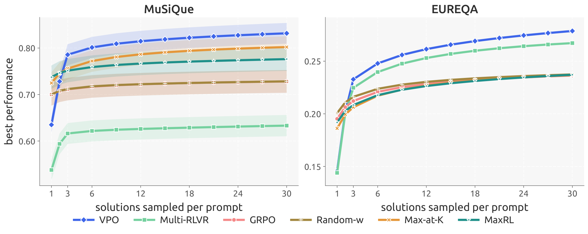
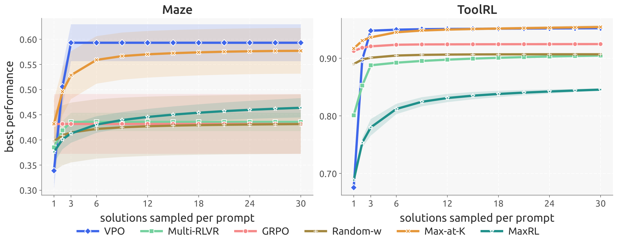
Across all four domains, Maze (Table 2), MuSiQue (Table 1), EUREQA (Table 3), and ToolRL (Table 4), VPO consistently improves best@ $k$ relative to scalar baselines. While scalar GRPO quickly saturates as $k$ increases, indicating collapsing candidate diversity, VPO continues improving with additional samples and plateaus at a substantially higher level. Figure 3 shows this effect on MuSiQue and EUREQA (the companion plot for Maze and ToolRL is in App. Appendix D).

\begin{tabular}{l c c c c c c}
\toprule
Method & best@ $3$ & best@ $5$ & best@ $10$ & best@ $30$ & F1@ $30$ & diversity \\
\midrule
Qwen3-1.7B (single-answer prompt) & $0.310$ & $0.339$ & $0.373$ & $0.423$ & $0.161$ & $0.634$ \\
 $\hookrightarrow$ GRPO & $0.711$ & $0.716$ & $0.721$ & $0.728$ & $0.447$ & $0.054$ \\
 $\hookrightarrow$ Random-w & $0.712$ & $0.716$ & $0.721$ & $0.728$ & $0.445$ & $0.061$ \\
 $\hookrightarrow$ Max-at-K & $\mathbf{0.757}$ & $\underline{0.768}$ & $\underline{0.783}$ & $\underline{0.802}$ & $\underline{0.573}$ & $0.175$ \\
 $\hookrightarrow$ MaxRL & $\underline{0.751}$ & $0.757$ & $0.765$ & $0.776$ & $0.552$ & $0.068$ \\
\midrule
Qwen3-1.7B (multi-answer prompt) & $0.402$ & $0.439$ & $0.475$ & $0.506$ & $0.379$ & $0.855$ \\
 $\hookrightarrow$ Multi-RLVR & $0.599$ & $0.616$ & $0.627$ & $0.633$ & $0.498$ & $\mathbf{0.814}$ \\
 $\hookrightarrow$ VPO (ours) & $0.742$ & $\mathbf{0.780}$ & $\mathbf{0.809}$ & $\mathbf{0.832}$ & $\mathbf{0.678}$ & $\underline{0.587}$ \\
\bottomrule
\end{tabular}

\begin{tabular}{l c c c c c}
\toprule
Method & best@ $3$ & best@ $5$ & best@ $10$ & best@ $30$ & diversity \\
\midrule
Qwen3-4B (single-answer prompt) & $0.341$ & $0.457$ & $0.596$ & $0.714$ & $0.905$ \\
 $\hookrightarrow$ GRPO & $0.432$ & $0.432$ & $0.432$ & $0.432$ & $0.003$ \\
 $\hookrightarrow$ Random-w & $0.414$ & $0.420$ & $0.425$ & $0.432$ & $0.090$ \\
 $\hookrightarrow$ Max-at-K & $\mathbf{0.526}$ & $\underline{0.552}$ & $\underline{0.568}$ & $\underline{0.577}$ & $\underline{0.671}$ \\
 $\hookrightarrow$ MaxRL & $0.414$ & $0.426$ & $0.441$ & $0.464$ & $0.206$ \\
\midrule
Qwen3-4B (multi-answer prompt) & $0.066$ & $0.103$ & $0.178$ & $0.334$ & $0.176$ \\
 $\hookrightarrow$ Multi-RLVR & $0.420$ & $0.430$ & $0.435$ & $0.436$ & $0.187$ \\
 $\hookrightarrow$ VPO (ours) & $\underline{0.512}$ & $\mathbf{0.564}$ & $\mathbf{0.591}$ & $\mathbf{0.593}$ & $\mathbf{1.006}$ \\
\bottomrule
\end{tabular}

```latextable {caption="Table 3: Best@ k on EUREQA (held-out half of hard_5, averaged over 4 evaluation seeds)."} \begin{tabular}{l c c c c c} \toprule Method & best@ $3$ & best@ $5$ & best@ $10$ & best@ $30$ & diversity \ \midrule Qwen3-8B (single-answer prompt) & $0.081$ & $0.096$ & $0.117$ & $0.153$ & $0.171$ \ $\hookrightarrow$ GRPO & $0.212$ & $0.219$ & $0.226$ & $0.236$ & $0.119$ \ $\hookrightarrow$ Random-w & $\mathbf{0.216}$ & $0.222$ & $0.229$ & $0.237$ & $0.105$ \ $\hookrightarrow$ Max-at-K & $0.206$ & $0.214$ & $0.224$ & $0.237$ & $0.140$ \ $\hookrightarrow$ MaxRL & $0.209$ & $0.216$ & $0.224$ & $0.237$ & $0.117$ \ \midrule Qwen3-8B (multi-answer prompt) & $0.102$ & $0.113$ & $0.126$ & $0.140$ & $0.171$ \ $\hookrightarrow$ Multi-RLVR & $0.210$ & $\underline{0.230}$ & $\underline{0.249}$ & $\underline{0.267}$ & $\mathbf{0.526}$ \ $\hookrightarrow$ VPO (ours) & $\underline{0.213}$ & $\mathbf{0.236}$ & $\mathbf{0.257}$ & $\mathbf{0.279}$ & $\underline{0.512}$ \ \bottomrule \end{tabular}


```latextable {caption="Table 4: Best@ k on ToolRL (80-prompt held-out split, averaged over 4 evaluation seeds)."}
\begin{tabular}{l c c c c c}
\toprule
Method & best@ $3$ & best@ $5$ & best@ $10$ & best@ $30$ & diversity \\
\midrule
Qwen3-1.7B (single-answer prompt) & $0.112$ & $0.114$ & $0.116$ & $0.123$ & $0.026$ \\
 $\hookrightarrow$ GRPO & $\underline{0.921}$ & $0.923$ & $0.924$ & $0.925$ & $0.044$ \\
 $\hookrightarrow$ Random-w & $0.902$ & $0.904$ & $0.906$ & $0.907$ & $0.064$ \\
 $\hookrightarrow$ Max-at-K & $\mathbf{0.940}$ & $\mathbf{0.945}$ & $\underline{0.949}$ & $\mathbf{0.954}$ & $0.131$ \\
 $\hookrightarrow$ MaxRL & $0.779$ & $0.805$ & $0.826$ & $0.846$ & $\underline{0.510}$ \\
\midrule
Qwen3-1.7B (multi-answer prompt) & $0.093$ & $0.104$ & $0.111$ & $0.116$ & $0.198$ \\
 $\hookrightarrow$ Multi-RLVR & $0.861$ & $0.883$ & $0.898$ & $0.905$ & $0.308$ \\
 $\hookrightarrow$ VPO (ours) & $0.897$ & $\underline{0.934}$ & $\mathbf{0.950}$ & $\underline{0.952}$ & $\mathbf{1.297}$ \\
\bottomrule
\end{tabular}

Is the gain due to multi-answer prompting alone?

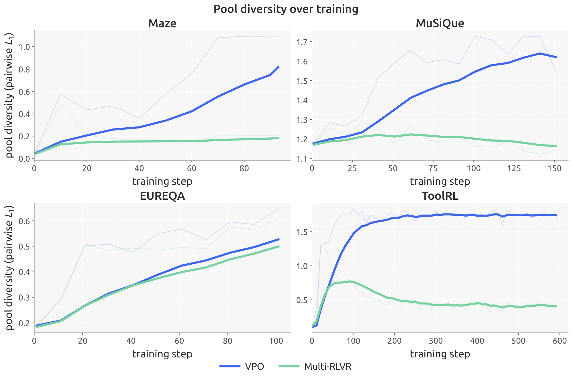
We want to understand if generating multiple answers within a shared autoregressive context, as explored in ([20]) is enough for diversity. It does not. VPO outperformed Multi-RLVR on best@ $k$ across all four domains, and the gap widened with $k$, mirroring the pattern against scalar GRPO. The mechanism is visible in App. Appendix D, Figure 6, which plots the pairwise $L_1$ distance between the per-rollout reward vectors in each candidate pool—a measure of how much the pool spreads in reward space, not in token space. Throughout training, Multi-RLVR's reward-space diversity collapses on Maze, MuSiQue, and ToolRL. Interestingly, the domain on which Multi-RLVR performs best relative to the other baselines (EUREQA) is also the only one on which its training-time reward-space diversity tracks VPO's, supporting the hypothesis that VPO's training-time diversity is instrumental in improving test-time performance. We conclude that multi-answer prompting supplies the capacity to produce distinct candidates, but under a fixed scalarization, the gradient still pushes every position in the chain toward the same scalar optimum, so the candidates collapse to similar reward vectors. The stochastic scalarization in VPO gives different positions an incentive to specialize.

Is the gain due to more evaluator signal during training or normalization issues?

\begin{tabular}{l c c}
\toprule
Method & best@3 & $\mathbb{E}_w$ [best@3] \\
\midrule
GRPO ($n{=}8$) & 0.741 & 0.830 \\
GDPO ($n{=}8$) & 0.737 & 0.832 \\
GRPO ($n{=}24$, 3 $\times$) & 0.763 & 0.841 \\
GDPO ($n{=}24$, 3 $\times$) & 0.765 & 0.850 \\
GRPO + rand- $w$ ($n{=}24$) & 0.755 & 0.839 \\
\textbf{VPO (ours, $n{=}8$)} & \textbf{0.779} & \textbf{0.856} \\
\bottomrule
\end{tabular}

Two natural questions arise. First, VPO may benefit simply from receiving 3x more evaluator signal per rollout. Second, GRPO is known to be sensitive to reward components with very different variances, where a single high-variance dimension can dominate the baseline-subtracted advantage. GDPO ([34]) addresses this by normalizing the advantage per reward dimension before aggregating. If VPO's gains came from better gradient conditioning across components rather than from set-level diversity, per-dimension normalization should close the gap.

We test both at once on the MuSiQue domain by giving GRPO and GDPO 3x the rollouts ($n=24$) to equalize evaluator calls with VPO at $n=8$. Note that this also gives the baselines 3x the LM compute, since their reasoning chains are independent per answer rather than shared, so the comparison is conservative against VPO. Table 5 shows that neither effect explains the gap. At matched $n=8$, GDPO closely tracks GRPO, indicating the per-component normalization is not a binding constraint. At 3x the compute, both GRPO and GDPO improve modestly but remain below VPO at $n=8$, and adding random $w$ scalarization at $n=24$ also fails to close the gap. Extra evaluator signal during training and better normalization help marginally, but scalarized objectives still remove the incentive to maintain a diverse candidate set.

Why not just condition on $w$?

\begin{tabular}{l c c c c}
\toprule
Method & best@ $3$ & best@ $6$ & $\mathbb{E}_w[\mathrm{best}@3]$ & $\mathbb{E}_w[\mathrm{best}@6]$ \\
\midrule
G.C.\, $w = w^\star$ & $\underline{0.205}$ & $\underline{0.205}$ & $\underline{0.201}$ & $\underline{0.201}$ \\
G.C.\, $w \sim \mathrm{Dir}(\textbf{1})$ & $\underline{0.205}$ & $\underline{0.205}$ & $\underline{0.201}$ & $\underline{0.201}$ \\
VPO (ours) & $\mathbf{0.512}$ & $\mathbf{0.576}$ & $\mathbf{0.512}$ & $\mathbf{0.584}$ \\
\bottomrule
\end{tabular}

To optimize the model to output responses on the Pareto front, VPO uses in-context exploration. Prior work instead trains goal-conditioned policies ([35, 36]) that take a target scalarization $w$ as input and optimize $w^\top r$ directly. (These approaches create diversity by varying $w$ at inference time). To compare, we train a goal-conditioned GRPO policy and evaluate it under two settings (Table 6): (i) conditioning on the canonical scalarization $w^*$ and (ii) conditioning on random $w\sim\mathrm{Dir}({\mathbf{1}})$. Neither matches VPO on the maze domain under either gold scalar expected value under a random weight distributions. Interestingly, the goal conditioned policy had mode collapsed (hence identical best@3 and best@6), and also began to ignore the conditioning. Despite explicit access to $w$, the model struggles to reliably translate text-encoded preferences into effective behavior.

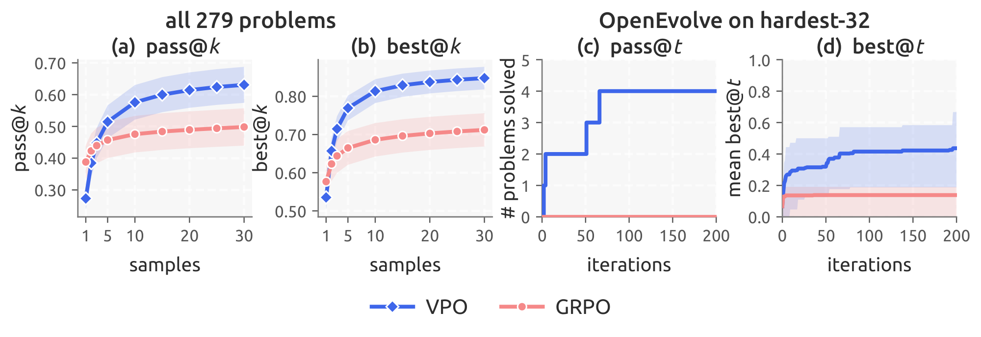
How does VPO scale to harder problems and more sophisticated search?

Two questions remain after the main results: does VPO's benefit survive on substantially harder problems, and does it survive under search procedures more sophisticated than best@ $k$? We answer both in a single-checkpoint case study comparing VPO to scalar GRPO on LiveCodeBench (LCB) ([37]), a competitive-programming benchmark with a strict temporal held-out cut (App. Appendix A.5). Both runs train on the same DeepCoder corpus from the same Qwen2.5-Coder-7B-Instruct checkpoint for one epoch; the only difference is the advantage estimator. On single-shot pass@ $1$ (Figure 4 A), the regime with no downstream search to amortize over, GRPO is better; the scalar baseline correctly wins when only one shot is allowed. The moment the model is given a candidate chain of $m{=}3$ and is evaluated under best@ $k$ (Figure 4 B), the picture inverts: VPO sits above GRPO at every $k$ and the gap widens with $k$, mirroring the main benchmark results. Replacing best@ $k$ with a more capable search procedure makes the case sharper still. We plug both checkpoints into OpenEvolve ([38]), an evolutionary test-time search loop that iteratively rewrites candidates against test feedback, and run it on the $32$ hardest held-out problems (those on which neither method passes any test case at best@ $30$). Over $200$ search iterations VPO continues to discover new solutions and cracks problems that neither arm could touch under the standard regime, while GRPO plateaus early (Figure 4 C, D). The case study points the same direction as the main results: diversity matters most when downstream search is non-trivial, and the benefit sharpens both as the problems get harder and as the search procedure gets more capable.

When would VPO not help?

VPO's central premise is that the reward decomposes into components whose individually optimal responses occupy distinct regions of the simplex, and its empirical gain is largest precisely when this premise holds. On Maze, MuSiQue, EUREQA, and ToolRL the on-policy reward components are not collinear under the trained model (see App. Appendix F), the Pareto front is wide, and VPO produces sets that span it. The benefit shrinks as the reward becomes effectively scalar. On a separate experiment using the UltraFeedback ([39]) under ArmoRM-5 reward model ([22]) the five nominally distinct components are near-collinear, and so the simplex collapses to a near-line, and VPO converges below scalar baselines on absolute best@ $k$ while still retaining the largest per- $K$ headroom of any method.

6. Related Work

Section Summary: Researchers have explored using LLMs inside search procedures that generate many candidate outputs and then pick the best one, as in best-of-N sampling or tree-of-thoughts methods, while other approaches modify training itself so that a model directly learns to produce sets of answers likely to contain a high-quality choice. Related efforts in multi-objective reinforcement learning randomize reward weightings during training to recover a range of useful behaviors, though standard RL fine-tuning tends to reduce output variety and thereby weaken performance when many samples are drawn later. VPO builds on these ideas by training a single policy to generate coordinated candidate sets that support selection across varying objectives.

Inference-time search over LLM outputs

A line of work treats the LLM as a generator inside a search loop. Best-of- $N$ sampling ([40]), self-consistency ([41]), particle filtering ([42]), and Tree-of-Thoughts ([43]) draw or expand many candidates and select among them. AlphaEvolve ([11]) and FunSearch ([44]) wrap static LLMs in evolutionary outer loops. The effectiveness of these approaches depends on generating candidate sets with sufficient diversity and quality for selection to improve outcomes. VPO instead trains the policy to directly produce candidate sets that better support inference-time selection. Another line of work integrate training into the search procedure ([45, 46]). These methods deliberately sacrifice generalization, as the policy is overfit to one instance for the duration of the search which is out of the scope of our setting.

Training for best@ $k$

A growing line of work modifies the training objective to anticipate inference-time selection. BOND ([47]) and BoNBoN ([48]) distill the Best-of-N distribution into a single policy. InfAlign ([49]) derives reward transformations that make standard RLHF inference-aware for procedures like BoN. Closer to our setting, BoN-aware fine-tuning ([50]), PKPO ([51]), Pass@ $k$ training ([5]), and max@ $k$ optimization ([32]) derive objectives that directly optimize max@ $k$ (or pass@ $k$ for binary rewards). These methods treat the $k$ samples as independent draws from the policy, whereas VPO emits the $m$ candidates as a single autoregressive chain. We additionally compare to Multi-RLVR ([20]), which jointly generates a set of $k$ outputs but optimizes a fixed scalar objective, whereas VPO optimizes across sampled reward weightings. Our experiments show that VPO outperforms these methods, including max@ $k$ training ([32]).

Multi-objective RL and reward randomization

Vector rewards and Pareto-optimal policy sets are classical tools in learning ([19, 25]). Goal-conditioned methods recover the Pareto front by training a single network conditioned on a sampled weight vector ([52, 53]). Reward randomization has also been used to escape local optima ([36]). [54] sample reward perturbations during training to discover diverse multi-agent strategies. VPO builds on these ideas and proposes an RL algorithm to optimize a multi-objective reward that fits and leverages the capabilities of LLMs.

Diversity collapse from RL post-training

RL post-training sharpens the output distribution and erodes pass@ $k$ at large $k$ ([17, 15, 18]). [16] argue this is structural. VPO instead changes the objective, so coverage of the reward simplex is the equilibrium rather than something a regularizer fights for.

7. Discussion and Conclusion

Section Summary: The core proposal is that language models used inside search-based systems should be trained to produce a broad, diverse set of competent answers rather than a single best one, leaving the search procedure itself to pick the most useful answer at runtime. VPO implements this idea by training on many different reward weightings so the model learns to cover the full range of trade-offs among competing objectives; experiments across several tasks show this yields stronger performance once search is allowed at test time, apparently because the training process preserves a wider variety of useful reasoning strategies. The method requires a multi-component reward signal and is intended only for settings that already perform test-time search; it also trades off single-answer accuracy for better coverage within a larger set of candidates.

We argued that when language models are deployed inside pipelines with test-time search, the responsibilities of exploration and exploitation should be separated: training should produce a diverse pool of competent candidates, and the search procedure at test time should handle exploitation. VPO instantiates this by sampling scalarizations uniformly over the simplex and training the policy to emit sets that span the Pareto front of the underlying reward components. The change is a drop-in replacement for the GRPO advantage estimator. Across MuSiQue, EUREQA, Maze, and ToolRL, VPO improves best@ $k$ over scalar baselines, with the gap widening as the test-time budget grows.

Why does VPO work?

We see two complementary explanations. First, policies that are optimized to maximize the set-level reward $R(S)$ may produce reward-diverse sets that cover the Pareto front (or its budget-constrained subset). The second possible explanation is about training dynamics. A candidate that scores poorly under $w^*$ but well under some other $w$ still receives a positive gradient on the rollouts where $w$ is sampled, while a fixed- $w^*$ run would push it away. VPO, therefore, could keep a broader set of reasoning strategies alive long enough to be refined, including strategies a $w^*$-trained policy would never visit. Although hard to measure, this could be a part of why VPO outperforms a $w^*$-trained policy even when both are evaluated under $w^*$.

Limitations

VPO comes with three limitations. First, precisely equalizing training compute across methods is non-trivial, since each method produces outputs of different lengths and VPO generates $m$ completions per rollout rather than one (though this is partly amortized because the reasoning prefix is shared across the $m$ solutions). To address this, we show in Section 5 that VPO continues to outperform GRPO on MuSiQue even when GRPO is given 3x the compute, indicating that the gains are not merely a function of compute mismatch. Second, VPO benefits from a vector-valued reward; when reward is scalar only, it reduces to more standard RL. Finally, it sacrifices pass@ $1$ for pass@ $k$ by training the policy to explore rather than to exploit. VPO is for the regime where test-time search is part of the system.

Acknowledgments

The authors express gratitude to Jyo Pari, Nitish Dashora, Andre Ye, Itamar Pres, Navodita Sharma, John Marangola, Nolan Fey, Oliver Sieberling, Linlu Qiu, Luca Grillotti, Benjamin Eysenbach, Yoon Kim, Jacob Andreas, and members of the Improbable AI lab at MIT for discussions that helped shape this work. This work was supported by National Science Foundation graduate research fellowships to RB, IP, and AK, the MIT-IBM Computing Research Lab, the MIT-Google Program for Computing Innovation and Hyundai Motor Company. This research was sponsored by the Army Research Office and was accomplished under Grant Numbers W911NF2110328 and W911NF-23-1-0277. The views and conclusions contained in this document are those of the authors and should not be interpreted as representing the official policies, either expressed or implied, of the Army Research Office or the U.S. Government. The U.S. Government is authorized to reproduce and distribute reprints for Government purposes notwithstanding any copyright notation herein.

Appendix

Section Summary: The appendix describes three experimental environments used to test the methods. The first is a 9x9 maze-generation procedure that creates graphs with controlled detours, item placements, and step budgets so that agents must choose among competing routes while avoiding obstacles, with rewards based on task completion plus fractions of gold collected, diamonds collected, and lava avoided. The second and third are multi-hop reasoning benchmarks: MuSiQue, which requires citing supporting paragraphs and composing answers across 2–4 hops amid distractors, and EUREQA, which presents a five-relation narrative chain of masked entities that the model must back-solve by name, both scored by vectors of binary correctness indicators plus answer quality.

A. Environment Details

A.1 Maze

Generation.

Each maze is a $9{\times}9$ grid built in two stages. We first carve a spanning tree using Prim's algorithm: starting from an all-walls grid and a uniformly random seed cell, we repeatedly pop a uniform random frontier cell and carve it to empty if it has exactly one empty neighbor (the standard wall-carving rule). We then inject $n_{\text{cycles}} \sim \mathrm{Unif}{18, \dots, 28}$ additional openings by converting wall cells with $\ge 2$ empty neighbors to empty; this is essential, since it turns the spanning tree into a multi-route graph so VPO's candidate pool has distinct paths to find. Endpoints are placed as one of ${(0, 0){\to}(8, 8), (0, 8){\to}(8, 0)}$ with equal probability; the remaining two corners are randomly designated the gold corner and diamond corner; the center cell $(4, 4)$ is a bonus tile that is rendered in the grid (as B) and advertised in the prompt as a score multiplier, but is in fact a distractor: visiting it has no effect on the reward. We then compute via-BFS detour lengths $\mathrm{via_gold} = d(S, \mathrm{gold}) + d(\mathrm{gold}, E)$, $\mathrm{via_diam} = d(S, \mathrm{diam}) + d(\mathrm{diam}, E)$, and $\mathrm{via_both} = d(S, \mathrm{gold}) + d(\mathrm{gold}, \mathrm{diam}) + d(\mathrm{diam}, E)$, and define the step budget $\text{budget} = \max(\mathrm{via_gold}, \mathrm{via_diam}) + 7$. We reject the maze unless $\mathrm{via_both} > \text{budget}$ – this is the design lever that guarantees the budget fits one corner detour but not both, so no single route can hit both the gold and diamond corners and still reach $E$. We then place $n_{\text{gold}} \sim \mathrm{Unif}{3, \dots, 5}$ gold cells in the Manhattan-radius-2 ball around the gold corner, the same for diamonds, and $n_{\text{lava}} \sim \mathrm{Unif}{3, \dots, 5}$ lava cells in the strict interior ${(r, c) : 2 \le r, c \le 6}$. A final BFS check verifies that a lava-avoiding path $S \to E$ exists within budget; otherwise the maze is rejected. The first 1000 mazes that survive (seeds from 42) form the train split; the next 100 (seeds from 4242) form the test split.

Reward.

The model's text output is parsed into a move list and simulated: walls and borders block, the trajectory ends as soon as $E$ is stepped on, lava is walkable but counted, and items only count if collected before reaching $E$. If $E$ is never reached, the reward vector is $(0, 0, 0, 0)$ on all four dimensions. Otherwise, define the per-item collection rates

$ g ;=; \frac{|\text{distinct gold visited}|}{n_{\text{gold}}}, \qquad d ;=; \frac{|\text{distinct diamond visited}|}{n_{\text{diam}}}, \qquad \ell ;=; 1 - \frac{|\text{distinct lava stepped}|}{n_{\text{lava}}}. $

The 4-D reward is

$ r(x, y) ;=; \bigl(, 1, ;, g, ;, d, ;, \ell, \bigr) \in [0, 1]^4, $

i.e., binary completion together with the three linear item-collection and lava-avoidance fractions. The gold scalar used by GRPO, MaxRL, GoalCond($w^\star$) training, and by best@ $k$ evaluation is the uniform mean

$ \bar{r} ;=; \tfrac14 \bigl(r_1 + r_2 + r_3 + r_4\bigr). $

A.2 MuSiQue

MuSiQue ([23]) is a multi-hop QA benchmark in which each 2–4 hop question decomposes into a chain of sub-questions whose answers must be composed; we use the MuSiQue-Ans split (19,938 train / 2,417 test). Each prompt embeds the question alongside 20 paragraphs, 2–4 of which carry gold supporting evidence and the rest sampled as distractors from MuSiQue's own paragraph pool (no external retrieval). The model emits a <support> block (paragraph indices, capped at four distinct entries) and an <answer> block. The reward vector $r(x, s) \in \mathbb{R}^5$ contains four binary citation indicators, one per gold hop ($\mathrm{hop}_1, \dots, \mathrm{hop}_4$), each ${0, 1}$ for whether <support> cites that paragraph, plus a continuous $\mathrm{answer_f1}$ against gold (best over aliases, with MuSiQue-style normalization: lowercase, drop articles, drop punctuation). The GRPO scalar is $\big(\sum_i \mathrm{hop}_i + 3, \mathrm{answer_f1}\big)/7$, weighting the answer $3\times$ to reflect that a correct answer is worth more than any single citation. The two reward components are causally linked but not redundant: a model can answer correctly while citing distractors, or cite correctly and fail to compose, so the domain probes pipeline coupling between evidence and answer. The asymmetric scalar weighting gives GRPO an explicit single-objective bias toward the answer, while vector-reward methods see all five dimensions at parity. We train Qwen3-1.7B from a shared base for one epoch across all methods and evaluate on a hop-stratified split of 300 held-out questions.

A.3 EUREQA

EUREQA ([30]) is a 5-hop chain-reasoning benchmark released with two difficulty levels of the same underlying questions: questions_normal_5 (1,109 examples, baseline phrasing) and questions_hard_5 (682 examples, harder rephrasings). We use a 50/50 random split of hard_5 (seed 0) as the held-out test set, and train on the remaining half of hard_5 together with all of the easier normal_5 rephrasings. The test set is therefore in-distribution with the harder half of training data, while the normal_5 rephrasings provide a small additional easy-data exposure. Each prompt is a narrative containing six masked entities $A, B, C, D, E, F$ connected by a 5-relation chain, with the anchor entity $F$ shown verbatim; the model must back-chain through the relations to identify $A$ through $E$ by their canonical Wikipedia names (e.g., Robert_Rodriguez), emitting five numbered tags. The reward vector $r(x, y) \in {0, 1}^5$ is binary, with one exact-match indicator per entity after Wikipedia-style normalization. The GRPO scalar is a uniform mean of the five dimensions. Unlike MuSiQue's loosely coupled hops, the EUREQA chain is causally chained: identifying $E$ requires composing a relation step from $F$, $D$ requires $E$, and so on. Scalar reward provides no signal about which hop in the chain failed, while vector-reward methods see per-hop correctness, so this domain probes whether per-dim training signal yields more robust chain-following on the harder rephrasings. We train Qwen3-8B and report best@ $k$ averaged over 4 evaluation seeds on the held-out hard_5 test split.

A.4 ToolRL

ToolRL ([24]) is a function-calling benchmark assembled from ToolACE, Hammer, and xLAM, comprising 3,920 train and 80 test prompts. The reward vector $r(x, y) \in \mathbb{R}^4$ contains one binary and three continuous F1 dimensions: $\mathrm{format} \in {0, 1}$ (structural well-formedness; all four format checks collapse to a single binary pass), $\mathrm{tool_name} \in [0, 1]$ (multiset F1 between predicted and gold tool-call names), $\mathrm{arg_key} \in [0, 1]$ (mean set-F1 over parameter keys across aligned tool calls, with greedy alignment by name then by key overlap), and $\mathrm{arg_value} \in [0, 1]$ (token-level F1 between predicted and gold values on aligned keys). The GRPO scalar is a uniform mean of the four dimensions. The dimensions are graded by difficulty: $\mathrm{format}$ is trivially solvable, $\mathrm{tool_name}$ requires retrieval, $\mathrm{arg_key}$ requires schema knowledge, and $\mathrm{arg_value}$ requires precise content generation. We train Qwen3-1.7B and report best@ $k$ averaged over 4 evaluation seeds on the 80-prompt test split.

A.5 LiveCodeBench (case study)

LiveCodeBench (LCB) ([37]) is a competitive-programming benchmark with a strict temporal held-out cut: each problem has a contest date and the held-out slice (Aug 2024 – Feb 2025) postdates every training-time problem, ruling out contamination by construction. We use LCB as a two-arm scaling case study (VPO and scalar GRPO only) rather than as one of the four main benchmark domains. Training data is the DeepCoder corpus, $24{,}269$ problems concatenated from three sources: $16{,}238$ from PrimeIntellect SYNTHETIC-1 (stdin, easiest), $7{,}432$ from TACO (Topics in Algorithmic Code Generation; verified competitive-programming slice, middle difficulty), and $599$ from LCB-v5 train (May – Jul 2024, hardest). Each row carries a structured array of test cases with inputs/outputs (and an fn_name field for functional-I/O problems); per-problem test counts are variable, capped at $32$ by the preprocessor. The held-out evaluation split is LCB-v5 Aug 2024 -- Feb 2025, $279$ problems, strictly later than every training-time LCB problem. The reward vector is a per-test-case binary pass indicator, $r(x, y) \in {0, 1}^{d}$, where $d$ is the problem-specific test count; VPO samples a Dirichlet of dimension $d$ per prompt with no zero-padding for advantage computation. The gold scalar is the uniform mean over the actually-present dimensions, which equals the problem's pass rate. Training uses Qwen2.5-Coder-7B-Instruct, FSDP across $8\times$ H100 80 GB, GRPO inner loop with PPO-clip $\varepsilon{=}0.2$, AdamW $\mathrm{lr}{=}10^{-6}$ (constant, no warmup), weight decay $0.01$, gradient clip $1.0$, KL coefficient $10^{-3}$, no entropy bonus; train batch $64$, mini-batch $32$, $n{=}8$ rollouts per prompt, generation temperature $0.8$, max context $4096 + 4096$. One epoch is $\approx 379$ steps; we evaluate at global_step_378 for both methods. The configuration is identical across VPO and GRPO except for the advantage estimator. For pass@ $k$ and best@ $k$ we sample $30$ candidates per problem at temperature $0.8$ over the full $279$-problem held-out split. For OpenEvolve we restrict to the $32$ hardest problems (those on which both VPO and GRPO score $0$ at best@ $30$ in the standard regime) and run $200$ iterations with $m{=}3$ candidates per iteration ($\approx 600$ candidates per problem); the test feedback from each iteration is exposed to the model as the search-loop input. The restricted subset isolates the regime where the standard best@ $k$ pool is exhausted, so any further progress must come from the search procedure itself rather than from drawing more samples.

B. Training Setup

All methods share a common GRPO ([13]) backbone implemented on top of veRL ([31]); only the advantage estimator changes per method. The recipe below applies to GRPO and to all VPO variants unless stated otherwise.

Advantage estimation.

For each prompt we sample a group of $n{=}8$ rollouts, compute a per-rollout scalar score (per-domain formula in Table 7), and form the advantage as the within-group $z$-score $\hat{A}_i = (\mathrm{score}_i - \mu_g)/(\sigma_g + \epsilon)$ with $\epsilon{=}10^{-6}$ and population standard deviation. The advantage is broadcast across all response tokens via the response mask. There is no value/critic network and no GAE.

Objective.

Standard PPO-clip with $\epsilon{=}0.2$ (symmetric, dual-clip $c{=}3.0$), $\mathrm{ppo_epochs}{=}1$, token-mean loss aggregation, and no entropy bonus. KL is applied as a loss-side regularizer only (no in-reward penalty): low-variance $k_3$ estimator against a frozen reference equal to the SFT initialization, with coefficient $\beta_{\mathrm{KL}} = 10^{-3}$.

Optimizer.

AdamW with learning rate $10^{-6}$, $(\beta_1, \beta_2){=}(0.9, 0.999)$, weight decay $0.01$, gradient clipping at $1.0$, no warmup, constant learning-rate schedule.

Engine and rollout sampling.

FSDP1 with bf16 mixed precision (parameter dtype fp32). The reference policy is a frozen copy of the actor's initialization with parameters CPU-offloaded between forward passes. Training rollouts use vLLM at temperature $1.0$, top- $p$ $1.0$, top- $k$ $-1$. In-training validation uses greedy decoding (do_sample=False) on all four domains as a low-noise progress signal.

Final-evaluation sampling.

The numbers reported in the main paper come from a separate post-training evaluation pass with stochastic decoding, so that best@ $k$ has a non-degenerate candidate pool to draw from. We use $\mathrm{top_k} = -1$ everywhere and the following per-domain settings, applied uniformly across every method evaluated on that domain: Maze and MuSiQue at temperature $0.7$, top- $p$ $1.0$; EUREQA and ToolRL at temperature $0.7$, top- $p$ $0.95$.

Per-domain batch sizes.

Batch sizes vary with model scale. For Qwen $\le$ 4B (Maze, MuSiQue, ToolRL): train batch $128$, mini-batch $64$, micro-batch $8$, $n{=}8$ rollouts per prompt. For Qwen 7B/8B (EUREQA): train batch $64$, mini-batch $32$, micro-batch $2$, $n{=}8$. We honor veRL's divisibility constraints (train $\times n$ divisible by GPU count; train divisible by mini-batch; mini-batch divisible by micro-batch $\times$ GPU count), so each PPO update consumes the full train-batch generation, with train $/$ mini gradient steps per generation.

Per-domain GRPO scalar.

Table 7 lists the per-domain scalar reward formulas $w^{\star\top} r(x, y)$ used as the GRPO score. Empty or unparseable responses receive $\mathrm{score} = 0$ in every domain.

\begin{tabular}{l c l}
\toprule
Domain & $d$ & GRPO scalar formula \\
\midrule
Maze & 4 & $\mathrm{mean}(\mathrm{completion}, \, \mathrm{gold}, \, \mathrm{diamond}, \, \mathrm{avoid\_lava})$ \\
MuSiQue & 5 & $\big(\mathrm{hop}_1 + \mathrm{hop}_2 + \mathrm{hop}_3 + \mathrm{hop}_4 + 3\, \mathrm{answer\_f1}\big)/7$ \\
EUREQA & 5 & $\mathrm{mean}(\mathrm{entity}_A, \mathrm{entity}_B, \mathrm{entity}_C, \mathrm{entity}_D, \mathrm{entity}_E)$ \\
ToolRL & 4 & $\mathrm{mean}(\mathrm{format}, \, \mathrm{tool\_name}, \, \mathrm{arg\_key}, \, \mathrm{arg\_value})$ \\
\bottomrule
\end{tabular}

C. Compute Resources

All experiments ran on NVIDIA H100 GPUs (80 GB SXM). Each training run used a single node with $4 \times$ H100, with a typical wall-clock duration of approximately 12 hours per run ($\sim$ 48 GPU-hours per run). The reported best@ $k$ numbers come from training one run per (method, domain) cell across the four domains (Maze, MuSiQue, EUREQA, ToolRL) and the five core methods (GRPO, Random- $w$, Max-at- $K$, Multi-RLVR, VPO), plus the goal-conditioned baseline on Maze and the $3{\times}$-rollout ablation on MuSiQue, totaling roughly 20–25 reported training runs ($\sim$ 1,000 GPU-hours). Including preliminary, failed, and hyperparameter-search runs, the full project consumed approximately $2\times$ the reported budget ($\sim$ 2,000 GPU-hours total). Inference-time evaluation (best@ $k$ pool generation and the $\bar\rho$ collinearity diagnostics in App. Appendix F) was orders of magnitude cheaper and is not separately accounted for.

D. Additional Figures

**Figure 5:** **Test-time scaling on Maze and ToolRL.** Best@ $k$ on the GRPO training scalar as a function of $k$, pooled across $c$ multi-answer chains per prompt. VPO matches or exceeds scalar baselines at every $k$ on Maze; on ToolRL all methods saturate near the reward ceiling and converge. Companion to Figure 3.

$**Figure 6:** **Reward-space diversity over training.** Pairwise $L_1$ distance between the per-rollout reward vectors $r(x, y) \in \mathbb{R}^d$ in each candidate pool, averaged across prompts, plotted over training steps. This measures the spread of the pool in reward space (not in token space): a large value means the rollouts realize different reward trade-offs. VPO sustains substantially higher reward-space diversity than Multi-RLVR throughout training; the only domain on which Multi-RLVR's diversity tracks VPO's is EUREQA, which is also the only domain on which Multi-RLVR comes close to VPO on best@ $k$.$

E. Domain Prompts

For each domain, we list the prompt template as it appears in the training corpus (single-solution form) followed by the rewriting applied for multi-solution methods (Multi-RLVR, VPO). We use $m{=}3$ candidates per multi-answer chain on all domains. Curly-braced names (question, m, etc.) are placeholders filled in per example. The goal-conditioning suffix (§ E.5) is appended only for the goal-conditioned baseline.

E.1 MuSiQue

Read the paragraphs below and answer the multi-hop question. Identify which paragraphs support your answer.

Paragraphs:
paragraphs_text

Question: question

First reason about which paragraphs are relevant, then output your supporting paragraph indices and answer.
<support>comma-separated paragraph indices (e.g., 3, 7, 12)</support>
<answer>your answer</answer>

paragraphs_text is "[idx] (Title: title) paragraph_text" joined over 20 paragraphs (2--4 gold, the rest distractors).

Multi-solution rewrite.

The block from First reason…'' through textless answertextgreater your answertextless/answertextgreater'' is replaced with:

Give m different answers in <response_i>...</response_i> tags, each with <support>indices</support> and <answer>answer</answer>.

The header, paragraphs, and question are unchanged.

E.2 EUREQA

You will be given a multi-hop reasoning question over a small narrative. The narrative contains masked entities (Person A, Country B, etc.) connected by relations. The leaf entity is revealed in the final sentence; you must back-chain to identify the rest.

Narrative:
narrative

The masked entities you must resolve (in order of introduction in the narrative):
mask_list

For each masked entity above, output its underlying canonical name. Use underscored Wikipedia-style names exactly as they appear in the source (e.g. `Robert_Rodriguez`, `32nd_European_Film_Awards`, `From_Dusk_till_Dawn:_The_Series`).

Replace each `...` below with the resolved entity (NOTHING else inside the tags — just the canonical name):
<entity_A>...</entity_A> (resolves mask_a)
<entity_B>...</entity_B> (resolves mask_b)
<entity_C>...</entity_C> (resolves mask_c)
<entity_D>...</entity_D> (resolves mask_d)
<entity_E>...</entity_E> (resolves mask_e)

The answer to the question is whatever you put in <entity_A>.

mask_list is the five masks bulleted with " - ".

Multi-solution rewrite.

The block from Replace each $\texttt{`...`}$ below…'' through … in textless entity_Atextgreater'' is replaced with:

Provide m different reasoning chains, each wrapped in numbered tags <response_1>...</response_1> through <response_{m}>...</response_{m}>. Each chain must contain all 5 entity resolutions; replace each `...` with ONLY the resolved canonical name (underscored Wikipedia-style, no prose, no labels):
  <response_i>
  <entity_A>...</entity_A> (resolves Person A --- this is the answer)
  <entity_B>...</entity_B> (resolves the second mask)
  <entity_C>...</entity_C> (resolves the third mask)
  <entity_D>...</entity_D> (resolves the fourth mask)
  <entity_E>...</entity_E> (resolves the fifth mask)
  </response_i>
Closing tags are required for every response and every entity. The m chains should be genuinely different attempts (e.g. different candidate resolutions, not paraphrases). The answer to the question is whatever you put in <entity_A> within each chain.

E.3 Maze

The example below shows the prompt for one specific maze (the per-maze grid, item counts, and step budget are filled in per example).

Navigate a 9x9 maze from S to E. Collect gold and diamonds, avoid lava.

Grid:
S . . . . . . D .
## . # . . . . D D

> **Section Summary**: The section describes a grid-based maze navigation task in which an agent starts at an implied position S and must reach exit E in at most 27 moves using only the four cardinal directions. The agent collects points from gold, diamond, and bonus tiles while avoiding lava, cannot pass through walls, and earns zero score if E is never reached or items are collected after arrival. A compact textual rendering of the grid is supplied along with an example output format for the required move sequence.

. . # # . . . . D
. # L . . . L # .
. . . . B . . . .
. . . . . L . . .
G . . . . . . . .
G G . . . . . . .
G G . . . . # . E

- Move: UP, DOWN, LEFT, RIGHT. # is a wall – you cannot enter it.
- Do not leave the grid.
- Collect: G (Gold), D (Diamond), B (Bonus) tiles by stepping on them.
- Avoid: L (Lava) tiles. Stepping on lava costs you.
- Visiting a B cell multiplies your other scores – explore!
- You MUST reach E. If you don't reach E, your score is zero everywhere.
- Items only count if collected BEFORE you reach E (the trajectory ends at E).
- You have 27 steps.

This maze has 5 Gold, 4 Diamond, 3 Lava, and 1 Bonus tiles.
Output moves in <answer>...</answer> tags, e.g., <answer>UP UP RIGHT</answer>.

Multi-solution rewrite.

The multi-solution prompt (used by VPO and Multi-RLVR with $m{=}3$) reuses the preamble, grid, and bullet list verbatim, except that You have 27 steps.'' becomes You have 27 steps per route.''. The closing two lines (the tile-count line and the ``Output moves …'' instruction) are replaced by the block below.

This maze has 5 Gold, 4 Diamond, 3 Lava, and 1 Bonus tiles.
Reason briefly about the maze, then provide 3 genuinely different routes from S to E.
Each route is a sequence of UP/DOWN/LEFT/RIGHT moves (space-separated).
Wrap each route in numbered tags (<route_1>...</route_1>, <route_2>...</route_2>,
<route_3>...</route_3>). Inside each tag put ONLY moves (no arrows, no coordinates,
no prose); any reasoning goes outside the tags. Each route has its own 14-step
budget and must reach E (score is zero if it doesn't).
Format example (m=3):
  <route_1>RIGHT RIGHT RIGHT RIGHT DOWN DOWN DOWN DOWN</route_1>
  <route_2>DOWN DOWN DOWN DOWN RIGHT RIGHT RIGHT RIGHT</route_2>
  <route_3>RIGHT DOWN RIGHT DOWN RIGHT DOWN RIGHT DOWN</route_3>

For general $m$, the tag list extends to < route_1>…</route_1>, …, < route_m>…</route_m>.

E.4 ToolRL

ToolRL prompts come directly from the upstream qiancheng0/ToolRL rlla_4k corpus: the system message specifies the output format and the user message contains the dialogue task. We do not override the system prompt.

You are a helpful multi-turn dialogue assistant capable of leveraging tool calls to solve user tasks and provide structured chat responses.

**Available Tools**
In your response, you can use the following tools:
1. Name: <tool_1_name>
Description: <...>
Parameters: {...}
2. Name: <tool_2_name>
...

**Steps for Each Turn**
1. **Think:** Recall relevant context and analyze the current user goal.
2. **Decide on Tool Usage:** If a tool is needed, specify the tool and its parameters.
3. **Respond Appropriately:** If a response is needed, generate one while maintaining consistency across user queries.

**Output Format**
<think> Your thoughts and reasoning </think>
<tool_call>
"name": "Tool name", "parameters": "Parameter name": "Parameter content", "... ...": "... ..."
"name": "... ...", "parameters": "... ...": "... ...", "... ...": "... ..."
...
</tool_call>
<response> AI's final response </response>

**Important Notes**
1. You must always include the `<think>` field to outline your reasoning. Provide at least one of `<tool_call>` or `<response>`. Decide whether to use `<tool_call>` (possibly multiple times), `<response>`, or both.
2. You can invoke multiple tool calls simultaneously in the `<tool_call>` fields. Each tool call should be a JSON object with a "name" field and an "parameters" field containing a dictionary of parameters. If no parameters are needed, leave the "parameters" field an empty dictionary.
3. Refer to the previous dialogue records in the history, including the user's queries, previous `<tool_call>`, `<response>`, and any tool feedback noted as `<obs>` (if exists).

The user message is the task itself, e.g.:

**Dialogue Records History**
<user> I need to make sure my library visit is smooth. Could you check if I'm a member, authorize my entry, log the access, and also verify the access control settings at the Main Library for the afternoon? </user>

Multi-solution rewrite.

The system message is unchanged. The block below is appended to the user message.

—
ADDITIONAL INSTRUCTION (overrides the single-attempt output format above): Provide m different attempts at the task. Wrap each attempt in numbered outer tags <response_1>...</response_1> through <response_{m}>...</response_{m}>. Inside each <response_i>, follow the original output format from the system prompt (your <think>, optional <tool_call>, and inner <response> sections). The m attempts should be genuinely different — different tool choices, different argument values, or different reasoning — not paraphrases. Closing tags are required on every outer attempt.

E.5 Goal-Conditioning Suffix (Goal-Conditioned GRPO baseline only)

For the goal-conditioned GRPO baseline (any domain), the following block is appended to whichever variant is in use (single or multi). Per training example, weights are resampled from $\mathrm{Dir}(1, \ldots, 1)$.

Your objective weights (higher = more important to optimize):
- desc_1: $w_1$:.2f
- desc_2: $w_2$:.2f
...

Maximize your weighted score.

The per-domain desc_i strings are domain-specific component names; for MuSiQue, e.g., "Finding evidence for reasoning step 1", …, "Finding evidence for reasoning step 4", "Answer word-level accuracy".

F. Reward Collinearity Predicts When VPO Helps

In § 5 we argued that VPO's gain over scalar baselines depends on whether the reward components are genuinely competing or effectively redundant. To make this prediction quantitative, we run a single cross-domain diagnostic: for each (domain, method) pair we measure (i) the on-policy collinearity of the reward vector under the trained model and (ii) the realized best@ $16$ under the GRPO training scalar. The prediction is that VPO outperforms scalar GRPO precisely when on-policy reward dimensions are not collinear; UltraFeedback should be the only domain in which the prediction inverts.

Table 9 confirms this. Across Maze, MuSiQue, EUREQA, and ToolRL, on-policy $\bar\rho$ stays well below 1 and VPO wins best@ $16$. On UltraFeedback the on-policy distribution is near-collinear ($\bar\rho_{\text{VPO}} = 0.95$, $\bar\rho_{\text{GRPO}} = 0.82$): the simplex collapses to a near-line, there is essentially one Pareto-optimal candidate per prompt, and VPO roughly matches GRPO. This is a sanity check on the regime claim in § 5: when the reward is effectively scalar, VPO does not (and should not) outperform scalar GRPO.

\begin{tabular}{l r r r r r r}
\toprule
Method & best@1 & best@5 & best@10 & best@20 & best@50 & $\Delta$ \\
\midrule
Qwen3-4B (single-answer prompt) & 0.700 & 0.724 & 0.730 & 0.735 & 0.741 & +0.041 \\
 $\hookrightarrow$ GRPO & \textbf{0.741} & $\underline{0.762}$ & $\underline{0.768}$ & $\underline{0.773}$ & $\underline{0.779}$ & +0.038 \\
 $\hookrightarrow$ GDPO & $\underline{0.737}$ & 0.759 & 0.765 & 0.770 & 0.776 & +0.039 \\
 $\hookrightarrow$ Goal-cond & 0.727 & 0.750 & 0.756 & 0.762 & 0.767 & +0.040 \\
\midrule
Qwen3-4B (multi-answer prompt) & 0.700 & 0.724 & 0.730 & 0.735 & 0.741 & +0.041 \\
 $\hookrightarrow$ Multi-RLVR & 0.730 & \textbf{0.763} & \textbf{0.770} & \textbf{0.775} & \textbf{0.780} & $\underline{+0.050}$ \\
 $\hookrightarrow$ \textbf{VPO (ours)} & 0.700 & 0.755 & 0.763 & 0.769 & 0.776 & \textbf{+0.076} \\
\bottomrule
\end{tabular}

\begin{tabular}{l c c c c c c}
\toprule
 & & \multicolumn{2}{c}{on-policy $\bar\rho$} & \multicolumn{2}{c}{best@16} & \\
\cmidrule(lr){3-4} \cmidrule(lr){5-6}
Domain & reward dims & VPO & GRPO & VPO & GRPO & $\Delta$ \\
\midrule
Maze & 4 reward feats ($D{=}4$) & 0.39 & 0.37 & \textbf{0.593} & $\underline{0.432}$ & \textbf{+0.161} \\
MuSiQue & 4 hop + 1 F1 ($D{=}5$) & 0.12 & 0.11 & \textbf{0.864} & $\underline{0.841}$ & \textbf{+0.023} \\
EUREQA & 5 entity-EM ($D{=}5$) & 0.05 & 0.03 & \textbf{0.204} & $\underline{0.182}$ & \textbf{+0.022} \\
ToolRL & 4 sub-metrics ($D{=}4$) & 0.86 & 0.62 & \textbf{0.953} & $\underline{0.924}$ & \textbf{+0.028} \\
UltraFeedback & 5 ArmoRM dims ($D{=}5$) & 0.95 & 0.82 & $\underline{0.767}$ & \textbf{0.772} & \textbf{-0.004} \\
\bottomrule
\end{tabular}

Methodology.

For each (domain, method) pair we proceed as follows.

On-policy rollout pool. Sample the trained checkpoint for that method on every prompt in the held-out evaluation set, drawing $N$ samples per prompt under the domain's final-evaluation sampler (App. Appendix B). Per-domain pool shapes (prompts $\times$ samples $\times$ reward dims) are: Maze $500\times30\times4$ ([completion, gold, diamond, avoid_lava]); MuSiQue $300\times30\times5$ (4 hop indicators + answer-F1); EUREQA $682\times50\times5$ (entity-EM); ToolRL $80\times N\times4$; and UltraFeedback (epoch 2) $200\times50\times5$ (ArmoRM dims).
$\bar\rho$ (on-policy off-diagonal Pearson correlation). Flatten the rollout tensor to $(N_{\text{responses}}, D)$, drop zero-variance dimensions, compute the $D{\times}D$ Pearson correlation matrix (np.corrcoef), and average the $D(D{-}1)$ off-diagonal entries. We report $\bar\rho_{\text{VPO}}$ and $\bar\rho_{\text{GRPO}}$ on the same prompt set under each domain's final-evaluation sampler.
Best@ $16$. Scalarize each response with the GRPO training scalar for that domain (per-domain formulas in Table 7; the ArmoRM "overall" dim for UltraFeedback). For each prompt, evaluate the unbiased order-statistic estimator of $\mathbb{E}[\max_{k \in S} r_k]$ over a uniform 16-element subset $S$ of the per-prompt sample pool, then average over prompts.

References

Section Summary: This section compiles a lengthy bibliography of academic papers, books, and preprints that support the article’s discussion. Most entries address core ideas in reinforcement learning, such as exploration techniques, intrinsic motivation, and multi-objective optimization, alongside recent studies applying these methods to large language models for improved reasoning, diversity, and test-time performance. Earlier foundational works sit alongside 2024–2026 preprints on LLM training, reward modeling, and evaluation benchmarks.

[1] Ladosz et al. (2022). Exploration in deep reinforcement learning: A survey. Information Fusion. 85. pp. 1–22.

[2] Sutton, Richard S and Barto, Andrew G (1998). Reinforcement learning: An introduction. MIT press Cambridge.

[3] Bellemare et al. (2016). Unifying count-based exploration and intrinsic motivation. Advances in neural information processing systems. 29.

[4] Pathak et al. (2017). Curiosity-driven Exploration by Self-supervised Prediction. arXiv:1705.05363 [cs, stat]. http://arxiv.org/abs/1705.05363.

[5] Chen et al. (2025). Pass@ k training for adaptively balancing exploration and exploitation of large reasoning models. arXiv preprint arXiv:2508.10751.

[6] Setlur et al. (2025). e3: Learning to explore enables extrapolation of test-time compute for llms. arXiv preprint arXiv:2506.09026.

[7] Qu et al. (2026). POPE: Learning to Reason on Hard Problems via Privileged On-Policy Exploration. arXiv preprint arXiv:2601.18779.

[8] Hong et al. (2024). Curiosity-driven red-teaming for large language models. In International Conference on Learning Representations. pp. 19935–19961.

[9] Cobbe et al. (2021). Training verifiers to solve math word problems. arXiv preprint arXiv:2110.14168.

[10] Brown et al. (2024). Large language monkeys: Scaling inference compute with repeated sampling. arXiv preprint arXiv:2407.21787.

[11] Novikov et al. (2025). Alphaevolve: A coding agent for scientific and algorithmic discovery. arXiv preprint arXiv:2506.13131.

[12] Lange et al. (2025). Shinkaevolve: Towards open-ended and sample-efficient program evolution. arXiv preprint arXiv:2509.19349.

[13] Shao et al. (2024). Deepseekmath: Pushing the limits of mathematical reasoning in open language models. arXiv preprint arXiv:2402.03300.

[14] Wu, Fang and Choi, Yejin (2025). The invisible leash: Why rlvr may not escape its origin. In 2nd AI for Math Workshop@ ICML 2025.

[15] Yang Yue et al. (2025). Does Reinforcement Learning Really Incentivize Reasoning Capacity in LLMs Beyond the Base Model?. https://arxiv.org/abs/2504.13837. arXiv:2504.13837.

[16] GX-Chen et al. (2025). KL-Regularized Reinforcement Learning is Designed to Mode Collapse. arXiv preprint arXiv:2510.20817.

[17] Robert Kirk et al. (2024). Understanding the Effects of RLHF on LLM Generalisation and Diversity. In The Twelfth International Conference on Learning Representations. https://openreview.net/forum?id=PXD3FAVHJT.

[18] Karouzos et al. (2026). Where does output diversity collapse in post-training?. arXiv preprint arXiv:2604.16027.

[19] Roijers et al. (2013). A survey of multi-objective sequential decision-making. Journal of Artificial Intelligence Research. 48. pp. 67–113.

[20] Puri et al. (2026). Reaching Beyond the Mode: RL for Distributional Reasoning in Language Models. arXiv:2603.24844 [cs]. doi:10.48550/arXiv.2603.24844. http://arxiv.org/abs/2603.24844.

[21] Chen et al. (2021). Evaluating large language models trained on code. arXiv preprint arXiv:2107.03374.

[22] Wang et al. (2024). Interpretable preferences via multi-objective reward modeling and mixture-of-experts. In Findings of the Association for Computational Linguistics: EMNLP 2024. pp. 10582–10592.

[23] Trivedi et al. (2022). MuSiQue: Multihop Questions via Single-hop Question Composition. Transactions of the Association for Computational Linguistics. 10. pp. 539–554.

[24] Qian et al. (2025). Toolrl: Reward is all tool learning needs. arXiv preprint arXiv:2504.13958.

[25] Hayes et al. (2022). A practical guide to multi-objective reinforcement learning and planning. Autonomous Agents and Multi-Agent Systems. 36(1). doi:10.1007/s10458-022-09552-y. http://dx.doi.org/10.1007/s10458-022-09552-y.

[26] Spector, Lee (2012). Assessment of Problem Modality by Differential Performance of Lexicase Selection in Genetic Programming: A Preliminary Report.

[27] Spector et al. (2024). Particularity.

[28] La Cava et al. (2019). A Probabilistic and Multi-Objective Analysis of Lexicase Selection and $\epsilon$-Lexicase Selection. Evolutionary Computation. 27(3). pp. 377–402. doi:10.1162/evco_a_00224.

[29] Ni et al. (2024). Dalex: Lexicase-like selection via diverse aggregation. In European Conference on Genetic Programming (Part of EvoStar). pp. 90–107.

[30] Li et al. (2024). Deceptive semantic shortcuts on reasoning chains: How far can models go without hallucination?. In Proceedings of the 2024 Conference of the North American Chapter of the Association for Computational Linguistics: Human Language Technologies (Volume 1: Long Papers). pp. 7675–7688.

[31] Guangming Sheng et al. (2024). HybridFlow: A Flexible and Efficient RLHF Framework. arXiv preprint arXiv: 2409.19256.

[32] Bagirov et al. (2025). The Best of N Worlds: Aligning Reinforcement Learning with Best-of-N Sampling via max@ k Optimisation. arXiv preprint arXiv:2510.23393.

[33] Tajwar et al. (2026). Maximum Likelihood Reinforcement Learning. arXiv preprint arXiv:2602.02710.

[34] Liu et al. (2026). GDPO: Group reward-Decoupled Normalization Policy Optimization for Multi-reward RL Optimization. arXiv:2601.05242 [cs]. doi:10.48550/arXiv.2601.05242. http://arxiv.org/abs/2601.05242.

[35] Yang et al. (2024). Rewards-in-context: Multi-objective alignment of foundation models with dynamic preference adjustment. arXiv preprint arXiv:2402.10207.

[36] Mahankali et al. (2024). Random latent exploration for deep reinforcement learning. arXiv preprint arXiv:2407.13755.

[37] Naman Jain et al. (2025). LiveCodeBench: Holistic and Contamination Free Evaluation of Large Language Models for Code. In The Thirteenth International Conference on Learning Representations. https://openreview.net/forum?id=chfJJYC3iL.

[38] Asankhaya Sharma (2025). OpenEvolve: an open-source evolutionary coding agent. https://github.com/algorithmicsuperintelligence/openevolve.

[39] Cui et al. (2023). Ultrafeedback: Boosting language models with scaled ai feedback. arXiv preprint arXiv:2310.01377.

[40] Ahmad Beirami et al. (2025). Theoretical guarantees on the best-of-n alignment policy. In Forty-second International Conference on Machine Learning. https://openreview.net/forum?id=u3U8qzFV7w.

[41] Wang et al. (2022). Self-consistency improves chain of thought reasoning in language models. arXiv preprint arXiv:2203.11171.

[42] Isha Puri et al. (2025). Rollout Roulette: A Probabilistic Inference Approach to Inference-Time Scaling of LLMs using Particle-Based Monte Carlo Methods. https://arxiv.org/abs/2502.01618. arXiv:2502.01618.

[43] Yao et al. (2023). Tree of thoughts: Deliberate problem solving with large language models. Advances in neural information processing systems. 36. pp. 11809–11822.

[44] Romera-Paredes et al. (2024). Mathematical discoveries from program search with large language models. Nature. 625(7995). pp. 468–475.

[45] Yuksekgonul et al. (2026). Learning to discover at test time. arXiv preprint arXiv:2601.16175.

[46] Wang et al. (2025). ThetaEvolve: Test-time Learning on Open Problems. arXiv:2511.23473 [cs]. doi:10.48550/arXiv.2511.23473. http://arxiv.org/abs/2511.23473.

[47] Sessa et al. (2025). Bond: Aligning llms with best-of-n distillation. In The Thirteenth International Conference on Learning Representations.

[48] Gui et al. (2024). Bonbon alignment for large language models and the sweetness of best-of-n sampling. Advances in Neural Information Processing Systems. 37. pp. 2851–2885.

[49] Balashankar et al. (2024). Infalign: Inference-aware language model alignment. arXiv preprint arXiv:2412.19792.

[50] Chow et al. (2025). Inference-Aware Fine-Tuning for Best-of-N Sampling in Large Language Models. arXiv:2412.15287 [cs]. doi:10.48550/arXiv.2412.15287. http://arxiv.org/abs/2412.15287.

[51] Walder, Christian and Karkhanis, Deep (2025). Pass@ K Policy Optimization: Solving Harder Reinforcement Learning Problems. arXiv preprint arXiv:2505.15201.

[52] Yang et al. (2019). A generalized algorithm for multi-objective reinforcement learning and policy adaptation. Advances in neural information processing systems. 32.

[53] Kanazawa, Takuya and Gupta, Chetan (2023). Latent-conditioned policy gradient for multi-objective deep reinforcement learning. In International Conference on Artificial Neural Networks. pp. 63–76.

[54] Tang et al. (2021). Discovering diverse multi-agent strategic behavior via reward randomization. arXiv preprint arXiv:2103.04564.