
DiffusionGemma Technical Report
DiffusionGemma Team
Google DeepMind$^{1}$
Abstract
We introduce DiffusionGemma, an experimental open-weight language model that uses discrete diffusion to generate text at exceptionally high speed. Rather than decoding one token at a time, DiffusionGemma iteratively refines blocks of 256 tokens in parallel, avoiding the sequential decoding bottleneck of conventional autoregressive (AR) large language models. Instead of training from scratch, we obtain DiffusionGemma by fine-tuning the mixture-of-experts Gemma 4 model with 3.8B activated and 25.2B total parameters. Our compute-efficient two-stage training pipeline uses fewer than 10% of the starting AR model's total training token budget. The first stage uses supervised fine-tuning to teach bidirectional denoising, while the second stage combines reinforcement learning with sampler distillation to jointly improve generation quality and inference efficiency. DiffusionGemma establishes a new Pareto frontier for the trade-off between generation speed and model capability. Averaged across our full evaluation suite, it generates around 20 tokens per forward pass and achieves roughly 1,500 output tokens per second on a single NVIDIA H100 GPU, which is substantially faster than AR models even with state-of-the-art speculative decoding. DiffusionGemma also retains the starting model's support for thinking mode, multimodal inputs, and long contexts. Despite diffusion fine-tuning, it remains capable of AR generation with only minor performance degradation, suggesting a path toward hybrid diffusion-AR decoding.
$^{1}$ Contributions, Acknowledgements and full author list: Page 38. Correspondence: [email protected].
Executive Summary: DiffusionGemma is an experimental open-weight language model developed by Google DeepMind that generates text using discrete diffusion instead of standard left-to-right autoregressive decoding. The work addresses a core limitation of current large language models: sequential token generation creates memory bottlenecks that slow single-user or low-concurrency requests, even when speculative decoding techniques are applied. Existing diffusion approaches were either closed behind APIs or lacked strong reasoning and multimodal capabilities while failing to deliver promised speed gains.
The team set out to produce a model that is simultaneously highly capable, exceptionally fast at inference, and freely accessible. They started from the publicly released Gemma 4 26B A4B mixture-of-experts checkpoint and applied a compute-efficient two-stage fine-tuning process that used less than 10 percent of the original model’s training tokens. The first stage used supervised fine-tuning to teach bidirectional denoising over blocks of 256 tokens. The second stage combined reinforcement learning with sampler distillation to improve output quality while sharply reducing the number of denoising steps required.
The resulting model generates roughly 20 tokens per forward pass on average and reaches about 1,500 output tokens per second on a single NVIDIA H100 GPU—roughly seven times faster than the Gemma 4 autoregressive baseline and nearly five times faster than the same model using multi-token prediction. It maintains competitive performance across reasoning, coding, multimodal, and agentic benchmarks while preserving support for thinking mode, long contexts, and multimodal inputs. It also retains the ability to run in standard autoregressive mode with only modest quality loss. These results establish a new operating point on the speed-versus-capability curve that surpasses both prior open diffusion models and the original autoregressive family.
The speed advantage is most pronounced in low-batch, latency-sensitive settings and opens practical routes to hybrid diffusion-autoregressive decoding that could route requests dynamically. The open Apache 2.0 release, together with reference implementations and a lightweight fine-tuning toolkit, lowers the barrier for domain-specific adaptation and further research.
Next steps should include targeted fine-tuning on specialized datasets, exploration of hybrid decoding strategies, and additional inference optimizations for higher batch sizes. Further work is also needed to close the remaining quality gap with the original autoregressive model and to reduce occasional repetitive outputs that appear under aggressive low-step sampling.
The main limitations are a modest performance trade-off relative to the starting autoregressive checkpoint, reduced output length, and throughput advantages that diminish beyond roughly 32 concurrent users. These findings rest on extensive benchmark coverage and controlled speed measurements, giving high confidence in the reported speed and capability results under the tested conditions.
1. Introduction
Section Summary: Autoregressive language models suffer from a memory bottleneck during low-concurrency use, as transferring weights and context to the accelerator takes far longer than computation itself, leaving hardware idle. Speculative decoding offers partial relief but remains limited by sequential drafting or falling acceptance rates, while existing text diffusion approaches are either proprietary, slow, or less capable. DiffusionGemma addresses these gaps by converting a pretrained Gemma 4 MoE model into a diffusion system that generates blocks of 256 tokens in roughly 12 passes, delivering around 1,500 tokens per second on one H100 GPU while preserving strong reasoning, multimodal, and long-context abilities through a lightweight two-stage adaptation process.
Autoregressive (AR) models dominate the current Large Language Model (LLM) landscape, but their strict left-to-right, token-by-token generation creates a problematic memory bottleneck. When serving many requests simultaneously, one can achieve acceptable throughput by batching, but serving single or low-concurrency requests is fundamentally memory-bound: time spent transferring model weights and context KV cache from memory to the accelerator far exceeds time spent on actual computation. This leaves the accelerator's compute units under-utilized and limits per-user generation speed. Speculative decoding can improve utilization by drafting a candidate sequence, typically 8 tokens, from a small "drafter" model and feeding the draft to the LLM for verification ([1, 2, 3]). With a draft length of 8 this can produce 3-6 tokens per forward pass (TPF) ([4]). However, the draft-then-verify paradigm is still limited: on one hand, AR drafters are bottlenecked by sequential generation; on the other hand, parallel drafters—building on early blockwise decoding ([5]) and lookahead strategies ([6])—exhibit declining acceptance rates at later draft positions ([7]).
Text diffusion circumvents this bottleneck by predicting entire blocks of tokens simultaneously (Figure 22), effectively shifting execution from a memory-bound regime toward a compute-bound one. Recently, there has been a surge of interest in text diffusion ([8]), with models like Gemini Diffusion ([9]), Mercury ([10]), LLaDA ([11, 12]), Seed Diffusion ([13]), and Nemotron-Labs-Diffusion ([14]). However, the current landscape forces a stark compromise between speed, intelligence, and accessibility. Some models, e.g., Gemini Diffusion and Mercury, are locked behind proprietary APIs. On the other hand, existing open-weights alternatives either exhibit limited reasoning capabilities and multimodal understanding, or fail to deliver on the extreme latency benefits promised by the diffusion technology, or both. Until now, there has been no text diffusion model that is highly intelligent, exceptionally fast, and openly accessible.

We introduce DiffusionGemma to bridge this gap. A finetuned text diffusion variant of the Gemma 4 26B A4B mixture-of-experts (MoE) model ([15]), the model establishes a new Pareto frontier in the intelligence-to-speed trade-off for generative text modeling (Figure 1). Notably, it extends the speed frontier beyond both prior text diffusion models and the Gemma 4 AR family across all parameter scales (from E2B up to 31B), even when the AR models are equipped with multi-token prediction (MTP, [16, 17]), a state-of-the-art speculative decoding technique. To unlock this new speed-to-intelligence frontier, DiffusionGemma maximizes algorithmic efficiency by outputting blocks of 256 tokens simultaneously in around 12 forward passes. Put differently, DiffusionGemma generates on average 20 TPF—a step-change improvement over the $\sim$ 3-6 TPF that can be achieved by state-of-the-art speculative decoding methods. This massive reduction in total forward passes directly offsets the computational cost of the diffusion model's heavier individual forward passes and as a result, DiffusionGemma yields generation speeds of around 1, 500 tokens per second (TPS) on a single NVIDIA H100 GPU. Furthermore, early benchmarking by third-party inference providers such as [18] demonstrates these speeds can scale up to 2, 000 TPS on the NVIDIA RTX 6000.
To avoid the prohibitive computational cost of pretraining it is common practice to initialize text diffusion models from pretrained AR models ([19, 20]). We warm-start DiffusionGemma from the final post-trained, publicly released weights of the Gemma 4 26B A4B MoE model ([15]). By adopting the same transformer backbone, we efficiently repurpose the AR weights to support both causal attention for context encoding and bidirectional attention for the diffusion process while inheriting their full capabilities. We employ a two-stage training pipeline (see Figure 2) that utilizes less than 10% of the AR model’s total training tokens:
- Supervised fine-tuning (SFT): We first run an SFT phase to adapt the model to attend to a context of clean tokens as well as denoising a block of 256 noisy tokens (as dictated by the diffusion process) with bidirectional attention across the block.
- Sampler distillation and reinforcement learning (SD $\cdot$ RL): We then apply an online learning phase that simultaneously improves generation quality (by maximizing rewards) and unlocks ultra-low latency (by substantially reducing the number of forward passes).
By preserving features of its AR starting point, DiffusionGemma exhibits strong multimodal understanding, long-context capabilities, and thinking mode, enabling it to generate reasoning traces prior to responding. These are hallmarks of current frontier systems ([21]). Although adapting the model to the diffusion regime introduces a performance penalty compared to the original AR baseline, the massive gains in inference speed offer an entirely new operating point for latency-critical applications. DiffusionGemma retains the ability to generate text autoregressively. This dual mode opens up the possibility to route requests dynamically based on latency constraints and task complexity, as well as to employ hybrid decoding approaches.
\begin{tabular}[t]{ll}
\toprule
Total & 25.2B \\
Activated & 3.85B \\
Vision Encoder & 550M \\
Embedder & 740M \\
Self-Conditioning & 7.8M \\
Active / Total Experts & 8 / 128 \\
  {} & + 1 shared \\
\bottomrule
\end{tabular}
\begin{tabular}[t]{ll}
\toprule
Canvas Length & 256 \\
Sampler Maximum Denoising Steps & 48 \\
Adaptive Stopping Entropy Threshold & 0.005 \\
Token Selection Entropy Threshold & 0.1 \\
Temperature Schedule (Linear) & 0.8 $\rightarrow$ 0.4 \\
\bottomrule
\end{tabular}
Open-weights release.
We release DiffusionGemma with open weights under a permissive Apache 2.0 license, aiming to democratize access to state-of-the-art text diffusion technology. By providing full, unrestricted access to the model parameters, we hope to empower a diverse ecosystem of researchers, developers, and practitioners. For the research community, this transparent release provides a robust, white-box baseline to deeply probe the underlying mechanics of discrete diffusion, accelerating foundational research and pushing the theoretical frontier of text generation. For developers, the liberal licensing removes friction, ensuring seamless integration into both experimental prototypes and commercial applications without restrictive usage barriers.
Crucially, DiffusionGemma's highly efficient architecture makes it an ideal foundation for rapid, domain-specific adaptation. By dramatically lowering the computational barrier to entry, the community can easily finetune ultra-fast, task-specific models tailored to their own unique use cases, even in environments with constrained compute budgets. This capacity for lightweight, rapid iteration has catalyzed immediate community adoption. Despite the model being available for only a few weeks at the time of writing, it is already serving as the engine for specialized downstream applications. These rapidly emerging use cases showcase the model's versatility across highly diverse and demanding domains, spanning from multilingual automatic speech recognition ([22]) to interactive radiology report drafting in healthcare ([23]).
Outline.
The remainder of this technical report is organized as follows. Section 2 formalizes the discrete diffusion framework and the theoretical foundations of our approach. Section 3 details the DiffusionGemma architecture, including the bidirectional decoding mechanism and sampling algorithm. We then describe the two stages of our training pipeline: the SFT phase in Section 4, followed by our online learning phase combining sampler distillation and reinforcement learning in Section 5. Section 6 breaks down our low-level inference optimizations. Section 7 presents experimental results. Section 8 provides instructions and a practical example of finetuning DiffusionGemma for downstream applications. In Section 9, we showcase some practical advantages of text diffusion. Finally, we discuss limitations and known issues in Section 10, before concluding in Section 11.
2. Generative Text Modeling with Discrete Diffusion
Section Summary: Traditional language models generate text one token at a time in a fixed left-to-right order, which constrains speed and prevents revising earlier choices based on later context. Diffusion approaches instead train a model to reverse a gradual noising process, iteratively refining an entire sequence in parallel from random noise. For discrete text tokens, continuous embedding-based diffusion methods encounter geometric and rounding problems that produce incoherent output, whereas native discrete diffusion models operate directly on categorical states through Markov transitions, providing a more grounded and effective path to high-quality parallel generation.
Historically, LLMs have treated text generation as a strictly sequential process ([24, 25, 26, 27, 28, 29]). Classical AR language modeling factorizes the joint probability of a sequence $x$ of length $L$ into an exact product of conditional probabilities: $p(x) = \prod_{i=1}^L p(x^i \mid x^{<i})$, where $i$ indicates the token position in the sequence. While theoretically rigorous, this single-token factorization fundamentally limits generation speed on modern hardware accelerators due to severe memory-bandwidth constraints as well as strictly preventing the model from bidirectionally revising tokens based on future tokens ([1, 30]).
Diffusion models approximate the joint distribution $p(x)$ by factorizing the generative process over a sequence of noise levels (a Markov chain) rather than strictly left-to-right spatial positions ([31, 32, 33, 34]), building upon foundational work in score-matching and continuous-time flow models ([35, 36, 37, 38, 39, 40]). During training, a forward process gradually corrupts clean data into random noise; a neural network is trained to learn the reverse denoising process. During inference, the model generates full sequences of data by iteratively refining the output sequence in parallel, starting from random noise.
Adapting diffusion to text requires handling the discrete nature of language ([41]). Early approaches adapt standard Gaussian diffusion to text by mapping discrete tokens into a continuous embedding space. These models differ primarily in how they map back to text: architectures like Diffusion-LM ([42]) and SED ([43]) produce continuous vectors that have to be forcibly projected or "rounded" back to discrete tokens, whereas methods like CDCD ([44]) maintain continuous processes but predict categorical logits directly to sample tokens. Regardless of the decoding mechanism, these formulations face theoretical and geometric challenges that ultimately limit their effectiveness compared to native discrete diffusion models. In particular, hard rounding operations fundamentally break exactness of diffusion likelihood bounds established by continuous-time and variational formulations ([45]) and the valid vocabulary tokens occupy an infinitesimally small fraction of a high-dimensional latent space. As a result, the reverse generative process often drifts into empty, "meaningless" regions of the space; when rounded to nearest token, these degenerate embeddings map to arbitrary, unrelated tokens and produce incoherent text ([46, 47]). To combat this spatial drift, methods have been developed to rely on per-step discretization mechanisms, but these generally underutilize the continuous space and restrict generative flexibility ([48]).
Discrete diffusion has emerged as a highly effective alternative ([49, 50, 51, 52]). This paradigm generalizes the single-step corruption heuristics of early bidirectional models into formal, multi-step Markov processes. The probabilistic transitions defined between categorical states in modern diffusion, such as absorbing mask states and multinomial distributions across the vocabulary, are direct descendants of masking and random token swapping introduced by BERT ([53, 54, 55]), as well as the plausible token replacements of ELECTRA ([56]). By operating directly on discrete states rather than continuous vectors, discrete diffusion avoids embedding projection mismatches entirely and offers better theoretical grounding for categorical transitions ([57]). DiffusionGemma builds upon this lineage of discrete diffusion to ensure high-fidelity token generation.
2.1 Probability Paths and Denoising
To formalize our discrete diffusion framework, we adopt the continuous-time Markov chain (CTMC) approach established in recent literature ([58, 59, 57]). Let $\mathcal{V}$ define a categorical token vocabulary of size $V$. We refer to the sequence of tokens undergoing iterative refinement as the canvas, with a length of $C$. A realization of this canvas at time $t \in [0, 1]$ is denoted by the vector $x_t \in \mathcal{V}^C$. We construct a marginal probability path to smoothly interpolate between a clean data distribution $p$ at time $t=0$ and a fully corrupted source canvas at time $t=1$. At the start of this path, the clean tokens are defined as $x_0 \sim p(\cdot)$, which ultimately transition into the fully corrupted state $x_1 \sim \operatorname{Unif}(\mathcal{V}^C)$. Here, $\operatorname{Unif}(\mathcal{V}^C)$ denotes the uniform prior over the joint state space, where each of the $C$ tokens is independently uniformly distributed over $\mathcal{V}$. This corruption process parallels the explicit transition matrices—such as uniform noise or absorbing masking—commonly utilized in order-agnostic discrete diffusion models ([60]). By operating in continuous time, this framework bypasses the sequential, left-to-right decoding bottleneck of traditional AR models, allowing tokens across the entire canvas to be processed and refined in parallel.
2.1.1 The Forward Process
The forward process dictates the transition from clean text tokens to uniformly distributed tokens. Conditioned on a fixed clean starting canvas $x_0$, the forward transition probability path factorizes independently over each token coordinate $i$:
$ \mathbb{P}(X_t=x_t \mid X_0 = x_0) = \prod_{i=1}^C \left[\kappa_t \delta(x_t^i, x_0^i) + (1 - \kappa_t) \frac{1}{V} \right],\tag{1} $
where $\kappa_t \in [0, 1]$ is a smoothly varying, monotonically decreasing noise schedule from $\kappa_0 = 1$ to $\kappa_1 = 0$, and $\delta$ represents the Kronecker delta. In practical terms, as time $t$ progresses toward $1$, each token is increasingly likely to be replaced by a token sampled uniformly at random from the vocabulary ([61, 49]). We use this closed-form forward process to generate training data from clean text.
2.1.2 The Backward Denoising Process
To reconstruct data from noise, we learn a reverse process to undo this categorical corruption. Discrete flow matching theory shows that to perfectly reverse the forward trajectory, we need to infer the conditional distribution of the original uncorrupted tokens given a corrupted state ([59, 57, 62]). For a given realization $X_t = x_t$, stepping backward in time by a small increment $\Delta t$ is governed by some transition mapping, which we denote $\operatorname{Step}$, which outputs the probability distribution for the next intermediate step[^2]:
[^2]: As a typical example, the function $\operatorname{Step}$ can be instantiated as a discrete Euler update step introduced in [57], in which $\mathbb{P}(X_{t-\Delta t}^i = v \mid X_t = x_t) \approx \delta(v, x_t^i) - \Delta t \frac{\dot{\kappa}_t}{1 - \kappa_t} \left[\mathbb{P}(X_0^i = v \mid X_t = x_t) - \delta(v, x_t^i) \right]$ with $\kappa_t \in [0, 1]$.
$ \mathbb{P}(X_{t-\Delta t} = \cdot \mid X_t = x_t) \approx \operatorname{Step}\Big(x_t, \mathbb{P}(X_{0} = \cdot \mid X_t = x_t)\Big).\tag{2} $
To compute this update, we need the true posterior distribution of clean tokens given a noisy state, $\mathbb{P}(X_{0}^i = v \mid X_t = x_t)$. We approximate this posterior with a neural network $p_\theta(v \mid x_t)$. During generation, we use this approximation to sample the next token state: $x_{t-\Delta t} \sim \operatorname{Step}(x_t, p_\theta(\cdot \mid x_t))$.
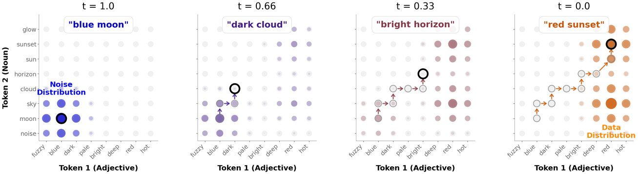
Figure 3 presents a highly stylized example to illustrate this reverse sampling trajectory within a simplified two-token canvas ($C=2$). As time runs backward from $t=1.0$ to $t=0.0$, the model smoothly shifts probability mass away from a uniform noise distribution (e.g., around "blue moon") toward valid data modes. Concurrently, individual sequence coordinates undergo continuous-time jump transitions—visualized by the step-by-step path from "blue moon" at $t=1.0$, to "dark cloud" at $t=0.66$, and finally landing on a high-probability mode like "red sunset" at $t=0.0$. This highlights how parallel dimensions coordinate over time without requiring sequential left-to-right generation.
Because this denoising process is factorized, it assumes conditional independence during individual reverse steps. A newly updated token at position $i$ is conditioned globally on the current noisy canvas $x_t$, but it cannot see the simultaneous sampling choices made at other positions ($j \neq i$). This structural tradeoff can occasionally introduce local inconsistencies or conflicting grammatical predictions. In the next section, we counteract these uncoordinated mechanics directly through our self-conditioning architecture and entropy-bounded sampling strategies.
3. The DiffusionGemma Architecture
Section Summary: DiffusionGemma is an encoder-decoder transformer initialized from an existing Gemma autoregressive model, allowing it to reuse pretrained weights for efficiency while supporting both diffusion-based generation and standard autoregressive sampling. At inference time it produces text in fixed-size blocks of 256 tokens by first encoding the prompt and prior output into a KV cache, then iteratively denoising a noisy canvas of tokens through a bidirectional decoder that attends to that cache. Once each canvas is clean it is encoded and appended to the cache, enabling scalable, long-form generation that combines the strengths of diffusion and autoregressive modeling.
The DiffusionGemma architecture functions as an encoder-decoder transformer ([28]) with shared weights $\theta$. Rather than pretraining a diffusion model from scratch, we initialize our model with the publicly released Gemma 4 26B A4B MoE checkpoint ([15]). Tying our architecture to an existing AR backbone is a pragmatic choice that trades off absolute generation quality for a substantial reduction in the computational cost of training. This initialization also allows us to inherit the base model's advanced features—such as its extended context window and native multimodal understanding. Moreover, our experiments demonstrate that our final model weights retain the ability to be sampled from autoregressively (see Table 3).
The remainder of this section details how DiffusionGemma uses this architecture to generate text at inference time. We break this process down into three components: the block-autoregressive decoding strategy for handling long sequences (Section 3.1), the general framework for denoising individual canvases (Section 3.2), and a specific entropy-bounded sampler (Section 3.3).
3.1 Block-Autoregressive Generation
The discrete flow matching formulation introduced in Section 2 operates on fixed-length sequences. To generate open-ended text, we use a block-AR generation strategy. The model denoises a canvas of 256 tokens at a time, and once a canvas is fully denoised, it is committed to the sequence history, and the model begins denoising the next canvas.
KV cache initialization.
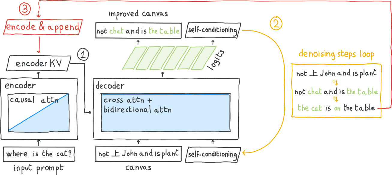
As illustrated in Figure 4, the first step in block-AR generation is to encode the context, $h \in \mathcal{V}^L$, into a KV cache $H$. The context includes system instructions and user prompts of maximum token count $L$.[^3] We write the encoding as
[^3]: In practice, $h$ also includes interleaved multimedia embeddings which are not part of the token vocabulary.
$ H = \operatorname{Encoder}_{\theta}(h),\tag{3} $
where $\operatorname{Encoder}_{\theta}$ is the transformer forward pass with weights $\theta$ and causal attention masking.
Canvas denoising conditioned on KV cache.
By cross-attending to the KV cache $H$, canvas generation can be conditioned on system instruction, user inputs and past responses. Canvas generation starts from a canvas of uniformly random tokens and is iteratively denoised using the process described in Section 3.2 and Section 3.3. Once a canvas is fully denoised, [^4] denoted by $\hat{x}_0$, its keys and values are appended to the KV cache (depicted in red in Figure 4):
[^4]: A canvas is fully denoised either by reaching $t=0$ or by the adaptive stopping condition described in Section 3.3.
$ H \gets H \oplus \operatorname{Encoder}_{\theta}(\hat{x}_0).\tag{4} $
We repeat this denoising process for subsequent canvases until the model generates a special token marking the end of the model's turn, after which all canvases $\hat{x}_0$ are concatenated into a final response. Since we use causal attention in the encoder, it lets the encoder update the KV cache by appending only the newest canvas. This constitutes an architectural inversion of standard encoder-decoder models such as BART ([63]) or T5 ([64]). Whereas those models utilize a bidirectional encoder for context and a causal decoder for generation, our approach utilizes a causal encoder for the sequence history and a bidirectional decoder for the diffusion-based canvas generation. This causal encoding prevents early context tokens from attending to the latest canvas, but it eliminates the need to re-encode the growing context from scratch, making our approach scalable to long reasoning generations and yielding a structural blend of diffusion and AR generation. This block-AR strategy was developed by our group in an unpublished June 2023 manuscript; analogous approaches to blockwise sequence modeling and KV caching were independently developed by [65], [66], and [67].
3.2 The Denoising Framework at Inference
Canvas initialization.
To generate a canvas, we iteratively refine it over a maximum of $N$ denoising steps, with step size $\Delta t = 1 / N$. Let $x_t \in \mathcal{V}^C$ denote the corrupted canvas at step $t$. We initialize the process at $t=1$ with a canvas $x_1$ of uniformly random tokens from the vocabulary $\mathcal{V}$.
The decoder forward pass.
At each step $t$, we apply the transformer with the shared weights $\theta$ as a decoder, written as $\operatorname{Decoder}_{\theta}$, to predict the probability distribution of the clean tokens. The decoder takes three inputs: the current noisy canvas $x_t$, the context KV cache $H$, and a continuous self-conditioning signal $z_t \in \mathbb{R}^{C \times d}$ that feeds the model's previous predictions back into itself ([68, 43, 69]). Using bidirectional attention across the canvas tokens and cross-attention to the KV cache, the decoder outputs the unnormalized logits $L_t$:
$ L_t = \operatorname{Decoder}_{\theta}(x_t, z_t, H) \in \mathbb{R}^{C \times V}.\tag{5} $
The denoising iteration.
At each iteration, we compute the logits $L_t$ and evaluate the clean token probabilities $\hat{p}_0$, update the self-conditioning signal for the next step, and sample the refined canvas:
$ \begin{aligned}\hat{p}0 &= \operatorname{Softmax} \big(L_t/\tau_t\big) \in [0, 1]^{C \times V}, \z{t-\Delta t} &= \operatorname{FFW}(\hat{p}0 E) \in \mathbb{R}^{C \times d}, \times{t-\Delta t} &\sim \operatorname{Step}(x_t, \hat{p}_0).\end{aligned}\tag{6} $
Here, $E \in \mathbb{R}^{V \times d}$ is the token embedding matrix and $\operatorname{FFW}$ is a standard feedforward network. The time-dependent temperature $\tau_t > 0$ can sharpen the model's predictions before we calculate the final transition probabilities. A transition mapping $\operatorname{Step}$, as described in Equation 2, computes the categorical distribution used to sample the updated canvas $x_{t-\Delta t} \in \mathcal{V}^C$, which, along with the new self-conditioning signal $z_{t-\Delta t}$, is then fed into the next denoising step. Section 3.3 details our specific choices for transition mapping $\operatorname{Step}$ and the temperature $\tau_t$.
Multinomial diffusion.
Our denoising iteration Equation (6) uses multinomial (or uniform) diffusion rather than masked diffusion ([61, 49]). Because all tokens can transition between one another, the model can continuously correct its own errors: tokens accepted during earlier denoising steps ($t' > t$) within the current canvas can still be revised. However, we note that tokens from previously generated canvases are permanently frozen.
Remark on interpretability.
Recent interpretability analyses demonstrate that while the self-conditioning signal $z_t$ introduces a continuous latent space injection into the sequence, these intermediate self-conditioning vectors map robustly to an interpretable token bottleneck, preserving the model's algorithmic transparency ([70, 71]).
3.3 The DiffusionGemma Sampler
In contrast to AR generation, which relies on rigid heuristics like temperature, top- $p$, and top- $k$, diffusion modeling introduces a vastly richer sampling design space that includes discrete predictor-corrector mechanisms and multi-step solvers ([72, 73, 74, 75, 76]). Framing text generation as an iterative temporal process allows us to decouple the inference-time algorithm from the underlying architecture, granting fine-grained control over the trade-off between computational cost and generation quality.
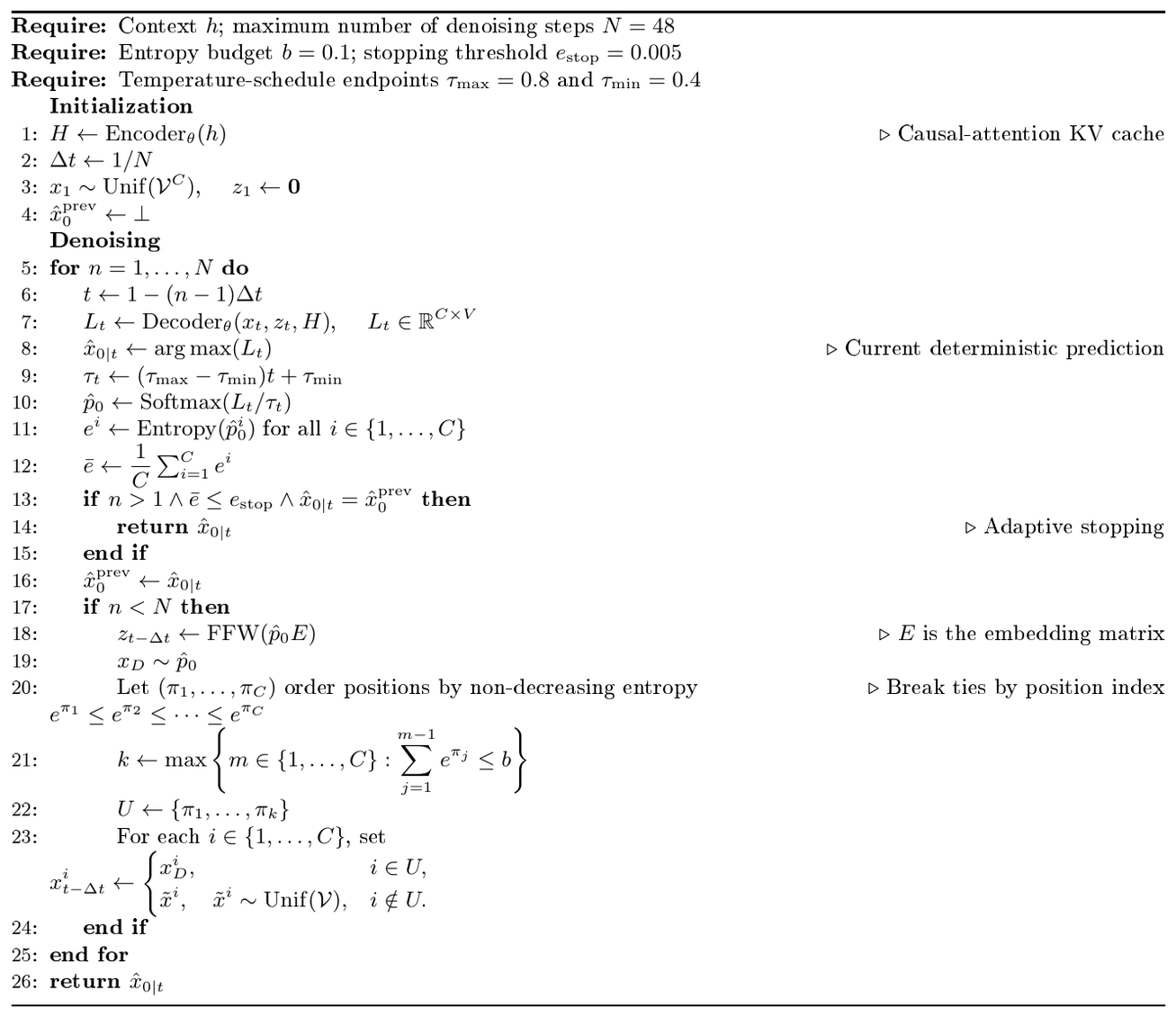
While we described the overall approach of canvas denoising in Section 3.2, this subsection details a specific instantiation: the entropy-bounded sampler ([77]) with temperature annealing and adaptive stopping (Algorithm 1). While this is our default and recommended sampler, DiffusionGemma is modular and is not strictly bound to this exact sampling configuration for high-quality inference.
Entropy-bounded token refinement.
After producing the marginal distributions $p_{\theta}(x_0 \mid x_t, z_t, H)$ with the denoiser and applying temperature scaling (detailed below), tokens are sampled from the resulting probability distribution. We employ an entropy-bounded sampler ([77]), whereby tokens are accepted in rank order from lowest to highest entropy (similar to the MaskGIT decoding scheme by [78]), ensuring that their mutual information bound remains strictly below a predefined error tolerance threshold ($b=0.1$). Once the threshold is attained, all other tokens are renoised uniformly at random, maintaining these uncommitted positions as a uniform prior to force local exploration during the next forward pass.
Temperature annealing.
To balance rate of convergence and linguistic diversity, token probabilities are artificially sharpened via tempering. A temperature $\tau_t < 1$ is annealed linearly from an initial value of $\tau_{\max}=0.8$ down to $\tau_{\min}=0.4$ across the fractional denoising timescale $t \in [0, 1]$. While static temperature adjustments are traditionally used to truncate the unreliable tail of token distributions and prevent text degeneration, this dynamic annealing ensures that the model explores diverse token possibilities in early, highly-noised states and aggressively commits to high-confidence sequences as the semantic structure crystallizes ([79]).
Adaptive stopping heuristic.
To optimize inference efficiency, the sampler dynamically halts the denoising process based on the model's step-wise uncertainty, strictly capping iterations at $N$. This early termination is triggered when two conditions are simultaneously satisfied:
- Confident predictions: The mean predictive entropy across the entire canvas falls below a predefined threshold ($e_{\mathrm{stop}}=0.005$).
- Stable predictions: The deterministic sequence predictions (i.e., the most likely tokens) from two consecutive denoising steps are identical.
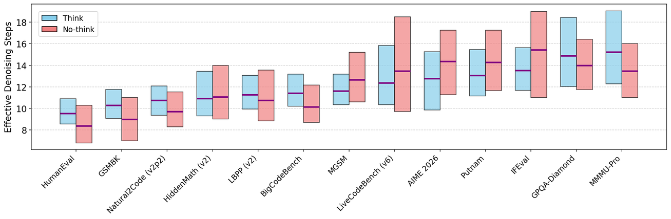
By successfully bypassing redundant refinement steps, this mechanism allows the model to dynamically scale its inference-time compute to the complexity of the prompt. As illustrated in Figure 5, instead of exhausting the maximum $N=48$ budget, the model averages approximately $12$ effective denoising steps (defined in Section 3.4) across the downstream evaluations shown in the figure. This yields a $4\times$ reduction in overall latency without sacrificing generation quality. Furthermore, the boxplots reveal distinct convergence profiles across domains: the model tends to deploy fewer steps for structured tasks like code and more for natural language. Moreover, it is not only the domain, but also the task complexity that dictates this behavior; for instance, harder code problems (e.g., LiveCodeBench) naturally require more steps to converge than easier ones (e.g., HumanEval).
3.4 Inference Efficiency Metrics
Because adaptive stopping turns the number of denoising steps into a random variable, we introduce a set of metrics to quantify denoising inference efficiency. Let $K$ be the total number of canvases generated, $N_k \leq N$ be the number of denoising steps executed for the $k$-th canvas, and $C_k \leq C$ be the number of valid tokens produced in that canvas (i.e., all $C$ tokens, or up to the first end-of-sequence token if one is generated). First, we define the Total Tokens as the sum of all valid tokens generated across the entire sequence:
$ \text{Total Tokens} \triangleq \sum_{k=1}^K C_k.\tag{7} $
We define the Total Denoising Steps as the absolute number of denoising steps executed across the entire generation:
$ \text{Total Denoising Steps} \triangleq \sum_{k=1}^{K} N_k.\tag{8} $
Since each denoising step incurs a fixed computational cost, the Total Denoising Steps is the primary driver of end-to-end generation latency. However, because this absolute metric inherently scales with the total sequence length, we also evaluate a normalized measure of model efficiency. We define the Effective Denoising Steps as the token-weighted average of steps across all canvases:
$ \text{Effective Denoising Steps} \triangleq \frac{1}{\text{Total Tokens}} \sum_{k=1}^K N_k C_k.\tag{9} $
We weight by the number of valid tokens to prevent the metric from being downwardly biased by the final canvas, which tends to require fewer denoising steps when it is only partially filled. Note that without adaptive stopping, the Effective Denoising Steps metric always reduces to the denoising budget $N$. Finally, we calculate the Tokens Per Forward (TPF):
$ \text{TPF} \triangleq \frac{\text{Total Tokens}}{\text{Total Denoising Steps} + K - 1},\tag{10} $
where the $K-1$ term accounts for the single additional forward pass required between canvases to encode the newly generated clean tokens and append their key-value pairs to the KV cache.
3.5 Retained Autoregressive Capability
Because DiffusionGemma shares the exact same transformer architecture as Gemma 4, the final DiffusionGemma weights can be seamlessly loaded back into the original architecture to perform standard AR generation using causal attention, exactly as the base model does. As demonstrated in Section 7, Table 3, the model maintains robust capabilities in this setting; its performance scores in AR mode land squarely between those of DiffusionGemma's primary text diffusion mode and the baseline Gemma 4 checkpoint from which DiffusionGemma was initialized.
4. Supervised Finetuning
Section Summary: They begin with the publicly released Gemma 4 26B model and continue training it to predict clean blocks of 256 tokens from partially noised versions of those blocks. During this supervised finetuning phase the model learns a block-wise denoising process that uses bidirectional attention inside each block while conditioning on the prompt and earlier clean blocks through a cached encoder state; training minimizes a standard cross-entropy loss on the original tokens. Early training quickly yields usable non-thinking performance, but longer training is required for stable thinking behavior, after which downstream accuracy improves in a steady log-linear pattern.
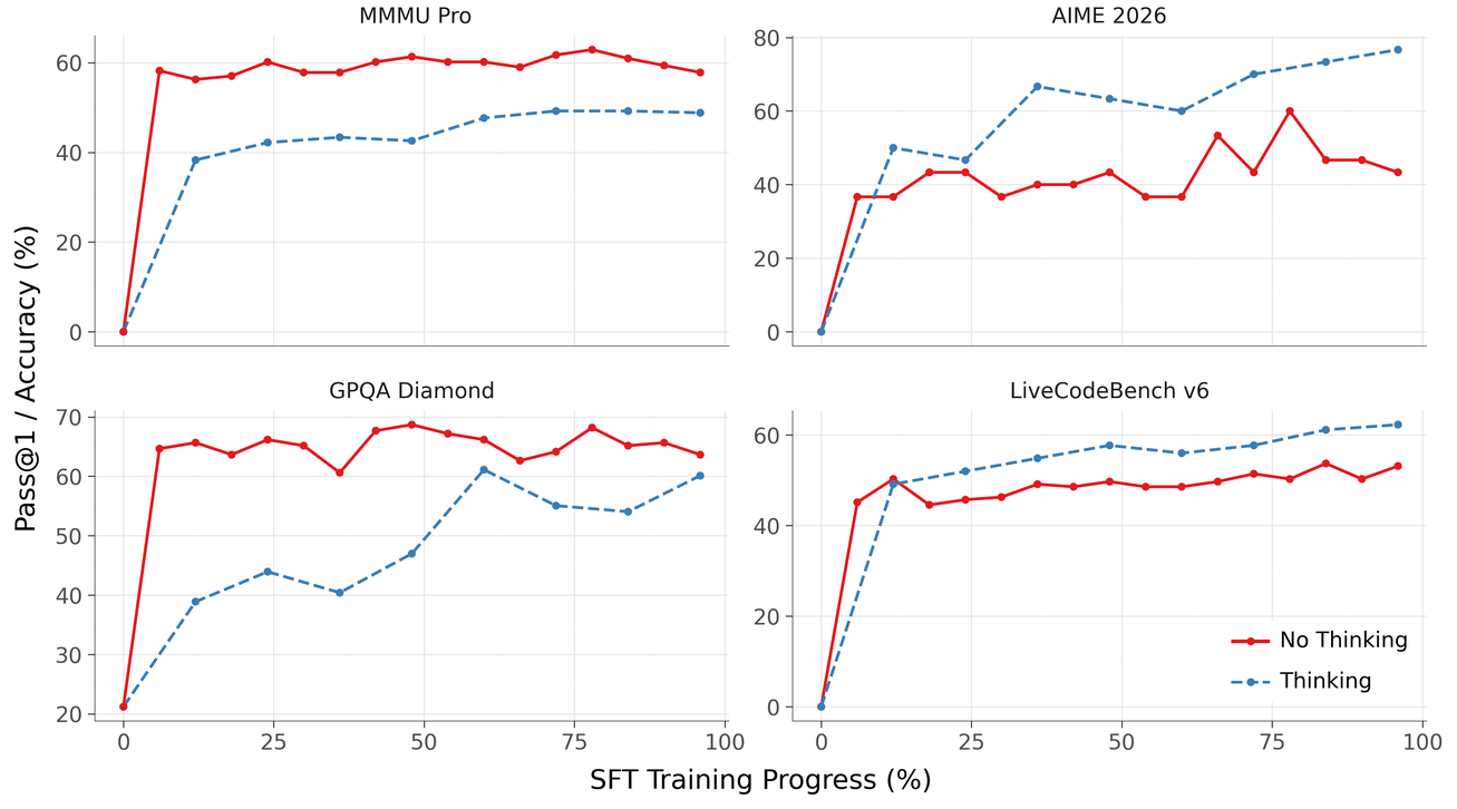
We start from the publicly released Gemma 4 26B A4B ([15]) checkpoint and run an extended finetuning phase where the model adapts to predicting blocks of 256 tokens from noisy inputs. We use a block-diagonal attention mask, enabling bidirectional attention within each block without allowing the model to condition on other denoising blocks. For a given canvas, the model conditions on the prompt and previous (uncorrupted) tokens via the encoder KV cache. We use discrete multinomial diffusion as our corruption process and uniformly sample noisy tokens from the vocabulary ([61, 49]). For a given canvas, we sample a noise level $t \sim \operatorname{Unif}[0, 1]$ and noise each token in the canvas with probability $t$. Given a clean context of prompt and previous canvases $H$ (encoded through the KV cache), a self-conditioning signal $z_t$, and a noisy canvas $x_t$, the model is trained to minimize the cross-entropy loss between its predictions and the ground-truth canvas extracted from the training data ([57]):
$ L(\theta) = - \sum_{i=1}^C \log p_{\theta}(x_0^i \mid x_t, z_t, H),\tag{11} $
where superscript $i$ denotes indexing along the canvas dimension; $p_\theta$ is parameterized via a softmax transformation over the neural network's output logits. As shown in Figure 6 and Figure 7, denoising performance improves rapidly within the initial steps of training, after which it settles into a log-linear performance improvement trend. Thinking performance benefits from extended SFT, as the model initially struggles with maintaining coherent reasoning traces, often collapsing into stuttering or cycles—a common challenge for internalizing reasoning in language models ([80]).
:::: cols="2"
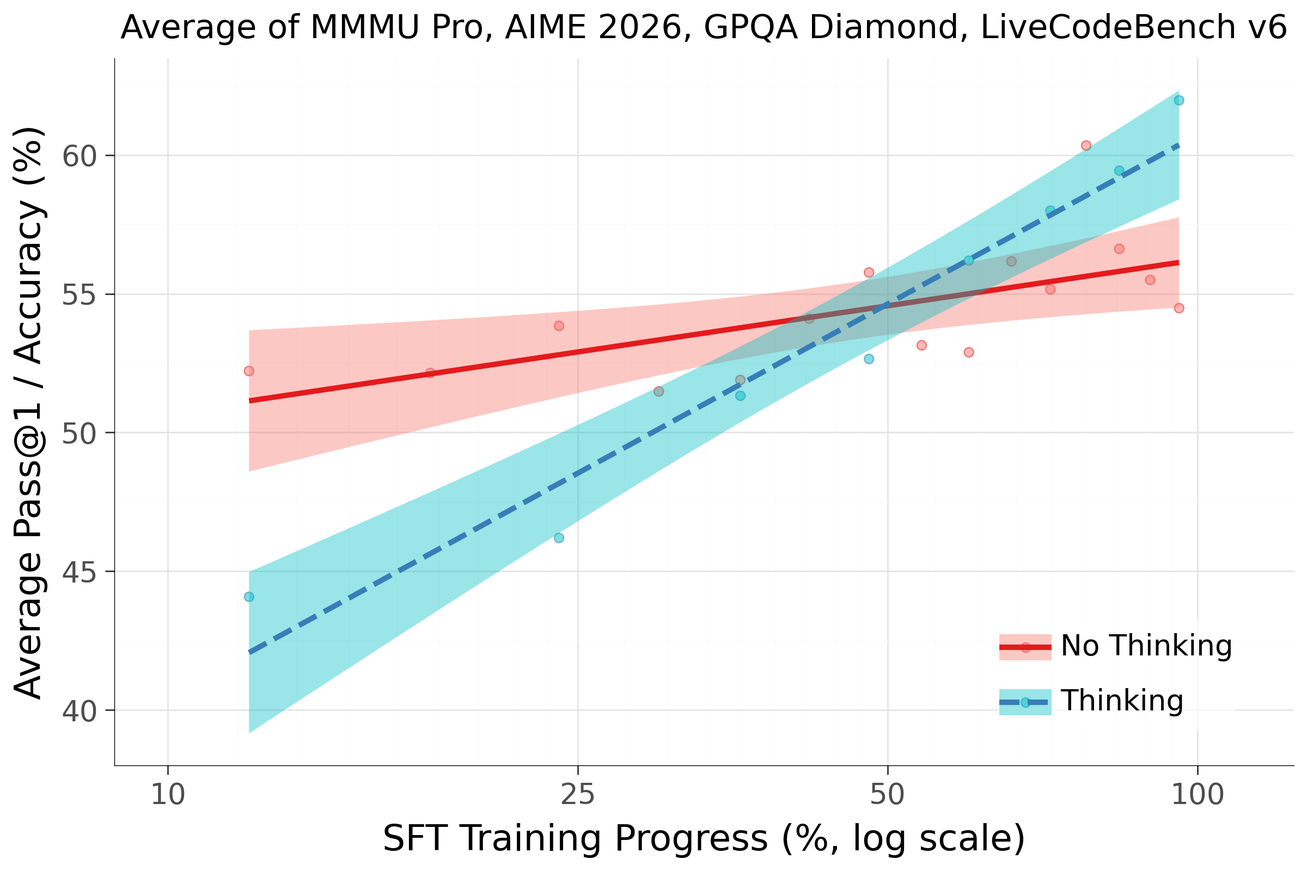
Figure 7: Downstream performance during SFT improves log-linearly with training progress. The log-linear trend for thinking performance starts off at a lower point yet exhibits a steeper slope than non-thinking mode. Results use the EntropyBounded sampler with adaptive stopping and a maximum of $N=192$ denoising steps.
::::
5. Sampler Distillation & Reinforcement Learning
Section Summary: After initial supervised training, the model produces high-quality results only with many denoising steps and struggles with fast, low-step inference or advanced reasoning tasks. To fix this, the authors introduce a single online training phase called sampler distillation and reinforcement learning that jointly raises output quality through reward maximization while compressing the best trajectories into a much smaller number of steps. This unified process creates an automatic curriculum that steadily improves both intelligence and speed, moving the model to a markedly better quality-versus-latency tradeoff.
Following the SFT stage, the model achieves strong generation quality when using a high number of denoising steps. However, its performance on advanced reasoning and coding tasks is somewhat poorer than the baseline AR model. More critically, when operating in the few-step regime required for ultra-low latency inference, generation quality collapses. To address this, we target a dual improvement: pushing the model's intelligence while simultaneously compressing its denoising trajectory.
Traditionally, achieving these two goals requires a decoupled, multi-stage pipeline that treats reward-driven alignment and sampler distillation as distinct phases. We bypass this with a unified online learning stage, coined sampler distillation & reinforcement learning (SD $\cdot$ RL), which optimizes both axes concurrently. Relying on a joint objective, a single gradient update drives:
- Reward maximization: Elevating absolute generation quality and alignment, analogous to standard RL for AR and diffusion models ([81, 82, 83, 84, 85, 86, 87, 88, 89, 90]).
- Sampler distillation: Mapping this high-quality generation to the few-step regime, addressing a compression challenge unique to iterative diffusion frameworks ([91, 92, 93, 94, 95, 96, 97, 98, 99]).
Training setup.
We adapt the data distribution used by the Gemma 4 RL recipe ([15]) for our use case. Encompassing both thinking and non-thinking modes, our setup targets improvements across a variety of capabilities such as helpfulness, mathematical reasoning, coding and instruction-following. Initialized from the SFT weights, the model acts as an online teacher that generates denoising trajectories (using a sampler configured with high maximum denoising steps and mild temperature annealing) to establish a high-quality reference. The SD $\cdot$ RL joint objective uses these trajectories to simultaneously maximize reward and drive sampler distillation in order to compress the model's highest-quality output into the few-step regime.
Training dynamics & implicit curriculum effect.
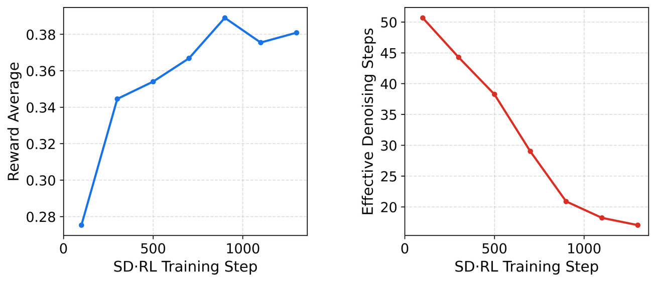
Over the course of SD $\cdot$ RL training, two synergistic dynamics emerge, as shown in Figure 8. First, the online teacher's average reward steadily increases, reflecting improved fundamental capabilities. Second, facilitated by the adaptive stopping mechanism, the online teacher progressively requires fewer effective denoising steps to achieve these high rewards. This acceleration occurs because the SD $\cdot$ RL objective systematically reduces the predictive entropy of the model. Crucially, the interplay between the reward objective and adaptive stopping induces a curriculum learning effect. Early in training, high predictive entropy delays the adaptive stopping trigger. As the model's confidence improves and entropy drops, adaptive stopping triggers earlier. This seamlessly shifts the training distribution toward ever shorter denoising trajectories, allowing the algorithm to dynamically pace its own sampler distillation. Consequently, and in contrast to RL for AR models, prolonging the SD $\cdot$ RL phase remains highly beneficial even after the reward metric plateaus; continued entropy reduction translates directly into further inference speedups.
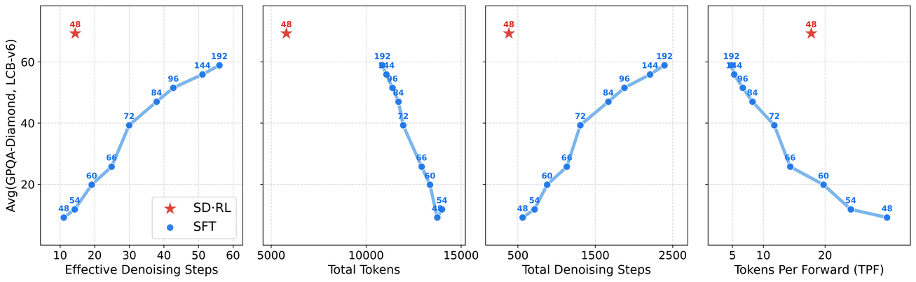
Improved speed-to-intelligence Pareto frontier.
As illustrated in Figure 9, SD $\cdot$ RL training significantly expands the Pareto frontier established by the SFT checkpoint. On the quality axis, it yields a 10-point improvement on the combined GPQA-Diamond and LiveCodeBench-v6 score. On the efficiency axis, it quadruples the TPF from 5 to nearly 20, unlocking ultra-low latency inference.
As shown in Figure 9, evaluating the SFT checkpoint with the default DiffusionGemma sampler (maximum of $N=48$ denoising steps) results in poor downstream accuracies and artificially low effective denoising steps. This counterintuitive behavior stems from the SFT model frequently degenerating into repetitive token loops in this restricted-step regime. Once it falls into a loop, its predictive entropy collapses, which prematurely triggers the adaptive stopping mechanism. Figure 16 and Figure 17 (Appendix C) provide generated samples on the GPQA-Diamond benchmark that illustrate how these degeneracies manifest: the SFT model begins with a valid, logical reasoning trace but suddenly collapses into a token repetition loop. In contrast, the samples post-SD $\cdot$ RL avoid these degenerative traps to sustain coherent reasoning at minimal latency.
SD $\cdot$ RL specialization in the few-step regime.
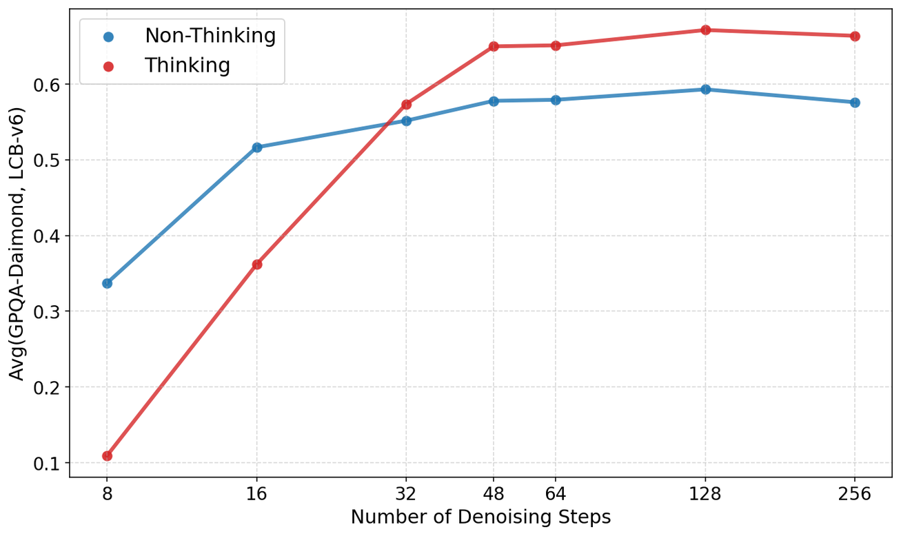
For the SFT checkpoint, downstream performance scales consistently with the maximum number of denoising steps $N$ up to 192, at which point denoising is roughly any-order autoregressive. Following SD $\cdot$ RL, the scaling behavior improves faster in $N$ and plateaus earlier: performance improves steadily up to $N=48$, but exhibits diminishing returns thereafter (Figure 10). This early saturation emerges because the SD $\cdot$ RL objective explicitly specializes the model for the few-step regime by aggressively minimizing predictive entropy.
Emergent conciseness.
An emergent property of our SD $\cdot$ RL optimization is that it encourages the model to produce concise, token-efficient outputs. This contrasts with RL for AR models, which often maximizes reward by inducing longer reasoning traces. Our final checkpoint produces generations nearly $2\times$ shorter than the SFT checkpoint (Figure 9). While this means the model forgoes some capability gains typically associated with extended reasoning, it acts as a multiplier on inference speed gains. Compounding fewer total tokens with fewer effective denoising steps per canvas directly drives exceptionally low end-to-end latency: DiffusionGemma requires less than $5%$ of the total forward passes used by the Gemma 4 AR baseline across our eval suite.
6. Inference Optimizations
Section Summary: The section explains how text diffusion models can achieve faster real-world inference than standard autoregressive models by minimizing the wall-clock time of each forward pass on GPUs, even though each step handles far more computation. Key optimizations include exploiting low-batch-size serving to reduce memory transfers, breaking down and addressing per-step bottlenecks in mixture-of-experts layers, sampling, and attention, and eliminating CPU-GPU synchronization through asynchronous scheduling. Together these yield a net throughput gain, with DiffusionGemma processing 256 tokens per step at only about 3.2 times the latency of a single-token baseline on hardware like the H100.
The preceding sections focused on maximizing the number of tokens produced per forward pass through our SFT and SD $\cdot$ RL pipeline. We now turn to the complementary axis: minimizing the wall-clock cost of each forward pass through targeted GPU-level optimizations. Fundamentally, the throughput advantage of text diffusion over AR decoding is dictated by two competing quantities: on one hand, each denoising step decodes $\mathrm{TPF}$ tokens, and thus requires $\mathrm{TPF}$ times fewer forward passes than an AR baseline. On the other hand, because each forward pass processes a canvas of 256 tokens, each such step is $r$ times slower, and so the overall throughput relative to the AR baseline becomes $\mathrm{TPF}/r$. The forward pass overhead can be substantially reduced by hardware optimizations.
Low batch size serving.
While text diffusion inference requires more floating-point operations (FLOPs) per generated token than AR models, it relies on significantly fewer forward passes. Because LLM serving on modern hardware accelerators is typically memory-bound—largely dictated by KV cache capacity and memory bandwidth ([100, 101])—this reduction in memory transfers creates a latency advantage that outweighs the higher computational cost. As a result, text diffusion is highly effective in low-batch-size scenarios, leveraging available compute capacity to minimize per-request latency. For simplicity, our analysis focuses on the single-request inference throughput (a batch size of 1) of DiffusionGemma, comparing it directly to its AR counterpart, Gemma 4 26B A4B. Reference inference implementations are available in HuggingFace Transformers ([102]) and vLLM ([103]).
GPU time breakdown.
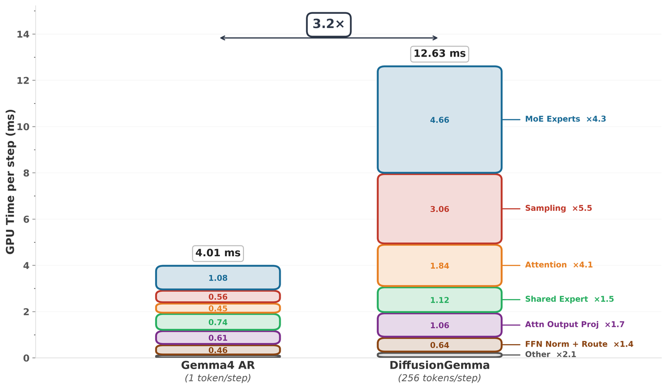
Figure 11 presents the per-step GPU kernel time breakdown for both models; we focus on GPU kernel time rather than end-to-end latency to isolate model-specific bottlenecks. For each model individually, end-to-end latency exceeds GPU kernel time by approximately 1 ms due to detokenization and other CPU-side serving overhead, with this gap being similar for both the Gemma 4 AR and DiffusionGemma models. Each DiffusionGemma step processes $256\times$ more tokens, yet is only $3.2\times$ slower than the single-token AR step. The time difference can be mainly attributed to three operations: mixture-of-experts (MoE), sampling, and attention. Other operations (e.g., shared expert, attention output projection, etc.) are at most $2\times$ slower.
- MoE. When serving a single request, the MoE layer computation is memory-bound, with its running time dominated by the transfer of expert weights from high-bandwidth memory, a well-documented bottleneck when serving sparse MoE models ([104, 105]). For the Gemma 4 AR model, only 8 unique experts are activated per token per MoE layer. For the DiffusionGemma model, on average, approximately 84 unique experts are activated per canvas of 256 tokens per MoE layer, as measured on the PG-19 benchmark ([106]).[^1] Activating more experts per forward pass results in a $4.3\times$ slower MoE kernel. It is the same type of penalty incurred by verification in speculative decoding, but scaled to larger token parallelism. For a dense architecture, this overhead would be eliminated, reducing the per-step feed-forward network slowdown to less than $2\times$.
- Sampling. Beyond AR's single-token softmax-and-sample, text diffusion sampling requires additional operations, most notably a self-conditioning embedding matmul and softmax over the full canvas of 256 tokens (see Algorithm 1). These operations are performed in full precision with a vocabulary dimension of 262k. Consequently, text diffusion sampling takes 3.06ms while AR sampling takes only 0.56ms. We implement sampling using standard PyTorch primitives optimized with
torch.compile, rather than hand-written GPU kernels, to facilitate easier extensibility by the community. - Attention. Unlike AR, DiffusionGemma uses bidirectional attention over a canvas of 256 tokens. As such, we cannot utilize the fast single-token decoding attention available to AR models, but we can take advantage of the highly-optimized FlashAttention-4 kernel ([107, 108]). Under these optimizations, the attention operation is $4\times$ slower for the DiffusionGemma model than the Gemma 4 AR model.
[^1]: Dataset available at https://github.com/google-deepmind/pg19.
Eliminating CPU-GPU synchronization.
There is additional complexity when serving DiffusionGemma: denoising steps depend on adaptive stopping and there are two types of forward passes (the denoising step and the KV cache update) that require different attention masks and that can occur within the same batch. To minimize request latency, it is important that this complexity is handled solely by GPU operations without triggering any additional CPU-GPU synchronization. This is achieved by extending asynchronous scheduling to the text diffusion models and introducing a per-sequence causal attention flag (see [103] for more details).
Throughput for batch size of 1 serving.
The decoding throughput for text diffusion models is calculated by the following formula:
$ \text{TPS} \triangleq \dfrac{\text{TPF}}{t_{\text{fwd}}},\tag{12} $
where TPS is Tokens Per Second, TPF is Tokens Per Forward (see Equation 10), and $t_{\text{fwd}}$ is the time needed for a single denoising step, which varies with context length (due to attention). On an H100 GPU (FP8 precision), a single denoising step of DiffusionGemma takes $t_{\text{fwd}}=13.56\text{ms}$ on average (end-to-end; the per-step GPU time is 12.63ms, see Figure 11) when serving a single request with 4096 input tokens and 1024 output tokens. TPF varies depending on the task. Assuming a TPF of 19.74 (the average TPF across the 7 benchmarks reported in Table 3), the average decoding throughput of the model is 1456 TPS—a $7.1\times$ improvement over the Gemma 4 AR model (204 TPS) and a $4.8\times$ improvement over the AR model with MTP (303 TPS), on the same device setup.
Multi-user throughput.
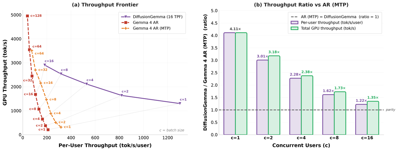
Figure 12 shows the trade-off between total and per-user throughput of the Gemma 4 AR model (with MTP) and DiffusionGemma depending on the number of concurrent users (i.e., batch size). Importantly, these results are without targeted optimization for batch sizes larger than 1: current kernel selection is suboptimal, and sampling has not been tuned to scale with batch size; for example, applying top- $k$ truncation to the sampling step is expected to yield significant throughput gains at higher batch sizes with negligible impact on output quality. Despite this, DiffusionGemma offers substantially higher TPS per user and higher total throughput than the Gemma 4 AR (MTP) model in the low batch size regime, with AR models beginning to gain a throughput advantage only at moderate batch sizes (around 32 concurrent requests).
Toward real traffic throughput.
Compared to the AR equivalent, DiffusionGemma changes the compute characteristics of two transformer layers: for the attention layer, it performs TPF $\times$ fewer transfers of KV cache; for the MoE layer, it performs proportionally more FLOPs (scaling with the number of effective denoising steps). This has the potential to address one of the challenges in modern LLM serving: memory-bound attention limiting compute utilization in FFW/MoE layers ([109, 110, 111]), which is particularly relevant for agentic workflows with long context. DiffusionGemma effectively trades data movement for compute, which is favorable on modern GPU hardware where compute-to-bandwidth ratios continue to grow; a thorough empirical analysis under realistic traffic conditions is beyond the scope of this work.
7. Experimental Results
Section Summary: DiffusionGemma was tested across math, coding, knowledge, and agentic benchmarks in both its text-diffusion and autoregressive modes, with and without an optional thinking step, and compared against its Gemma 4 starting point as well as other diffusion models. In diffusion mode it substantially beats existing open-source diffusion systems, matches the closed Mercury 2 model in quality, and reaches roughly 1,500 tokens per second on one H100 GPU—about 5 times faster than the original autoregressive baseline—while still supporting standard left-to-right generation when needed. The results show a clear speed-versus-accuracy trade-off that can be tuned by choosing the generation mode.
We evaluate DiffusionGemma's capabilities and inference efficiency across four operational modes: text diffusion (TD) versus autoregressive (AR) generation, each evaluated with and without thinking enabled; unless otherwise specified, TD with thinking is enabled. We benchmark the model against its AR initialization (Gemma 4 26B A4B), contemporary open-weight text diffusion models (LLaDA 2.1 Flash 100B and Nemotron Diffusion 14B), and the proprietary Mercury 2 API.
We consider a diverse suite of benchmarks spanning core domains such as mathematical reasoning, code generation, general knowledge, multimodal understanding, and instruction following alongside agentic capabilities. Specifically, for mathematical reasoning, we utilize AIME ([112]), GSM8K ([113]), MGSM ([114]), Putnam ([115]), and HiddenMath (internal). Coding performance is measured against LiveCodeBench-v6 ([116]), Codeforces ([117]), HumanEval ([118]), BigCodeBench ([119]), LBPP (v2) ([120]), and Natural2Code (internal). Broad and expert-level general knowledge is measured against GPQA-Diamond ([121]), BIG-Bench ([122]), MMMLU ([123]), and MMLU-Pro ([124]), while multimodal reasoning is evaluated on MMMU-Pro ([125]). Finally, strict instruction following is assessed via IFEval ([126]), and agentic task completion is evaluated through the Tau-bench suite, encompassing the Retail, Airline, and Telecom environments ([127]).
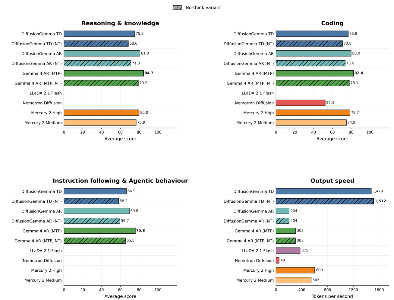
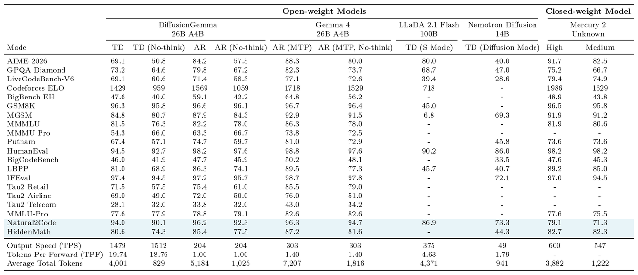
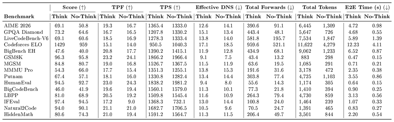
The complete per-benchmark results for all models and inference configurations are reported in Table 3. Table 4 provides a complementary analysis of DiffusionGemma's decoding efficiency, reporting Tokens Per Forward (TPF; Equation 10), Tokens Per Second (TPS; Equation 12), effective denoising steps Equation (9), total generated tokens Equation (7), and end-to-end generation latency, excluding prefill time. For a higher-level comparison, Figure 13 groups the benchmarks into three capability areas—reasoning and knowledge, coding, and instruction following and agentic behaviour—and reports the unweighted mean of the 0–100 benchmark scores within each area, together with output throughput. A model is shown for a capability area only if it completed every constituent benchmark; missing bars therefore indicate incomplete benchmark coverage rather than a score of zero. Hatched bars denote the no-think variants.
DiffusionGemma sets a new performance frontier for text diffusion models, substantially outperforming existing open-weight diffusion baselines while increasing TPF by approximately an order of magnitude. In terms of quality it is highly competitive with Mercury 2, a closed-weight text-diffusion model, while reaching roughly 1, 500 output tokens per second on a single previous-generation H100 GPU, a roughly $2.5\times$ speedup over Mercury 2.
Relative to the AR model used for initialization, DiffusionGemma in text-diffusion (TD) mode trades some absolute benchmark performance for substantially greater decoding speed. Although the conversion reduces performance across the three capability areas, TD mode delivers nearly $5\times$ the output throughput of the original Gemma 4 AR baseline under heavily optimized MTP serving: 1, 479 tokens per second compared with 303 tokens per second. The two-stage training pipeline nevertheless retains support for autoregressive decoding. When run in standard left-to-right AR mode, DiffusionGemma recovers part of the performance gap observed in TD mode and narrows the capability gap to the original baseline, albeit at lower throughput. This dual-mode capability could enable requests to be routed dynamically according to latency requirements and task complexity.
::: {caption="Table 3: Comparison of model performance, TPS and TPF across various benchmarks. TPS excludes prefill time; ' - ' denotes missing data. For speed measurements: DiffusionGemma and Gemma 4 are measured on 1 × H100 (FP8, batch size 1); Nemotron 14B on 1 × H100 (bfloat16, batch size 1); LLaDA 2.1 Flash 100B on 8 × B200 (bfloat16, batch size 1); Mercury 2 via its public API (see Appendix F for speed estimation). TPS, TPF and total tokens are averaged over the 7 benchmarks for which we have full coverage: AIME 2026, GPQA Diamond, LiveCodeBench-v6, MGSM, HumanEval, LBPP, and Natural2Code. TPS and TPF for Gemma 4 (MTP) are measured using SPEED-Bench ([128]). The Natural2Code and HiddenMath rows are highlighted as they are proprietary, unleaked evals."}
:::
::: {caption="Table 4: Performance and latency metrics of DiffusionGemma TD in Thinking vs. No-Thinking mode. We report accuracy/score, Tokens Per Forward (TPF, higher is faster), Tokens Per Second (TPS), Effective Denoising Steps (DNS, lower is faster), Total Forwards, Total Tokens, and End-to-End Latency per sample in seconds (excluding prefill time). The latency metrics are averaged across all samples within each benchmark."}
:::
8. Open-Source Downstream SFT
Section Summary: The authors release an open-source toolkit built on Hackable Diffusion that lets users adapt DiffusionGemma to their own datasets through parameter-efficient LoRA fine-tuning on modest hardware such as two A100 GPUs. The procedure combines a standard language-modeling loss over the full prompt-and-canvas sequence with a diffusion denoising loss on sampled canvases, optionally using self-conditioning, while LoRA is applied across attention, MLP, and router layers. As a demonstration, fine-tuning on Sudoku puzzles raises puzzle-solving accuracy from zero to roughly 84 percent while also cutting the number of required denoising steps.
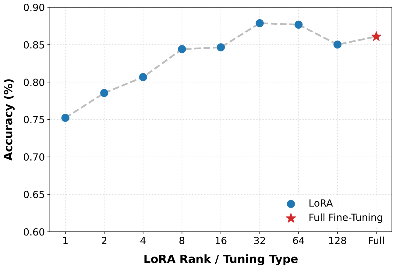
Alongside DiffusionGemma, we release an open-source finetuning toolkit that allows practitioners to adapt the model to their own domain-specific datasets. We build on top of Hackable Diffusion ([129]), a modular open-sourced research toolbox for generative modeling. We provide Low-Rank Adaptation (LoRA) recipes ([130]) to enable finetuning on consumer hardware.
Finetuning procedure.
Our open-source SFT toolkit includes both a causal encoder and a diffusion decoder objective. Training sequences are of length $P+KC$ where $P$ is the number of prompt tokens, $K$ is the number of canvases and $C$ is the canvas size. To compute the total loss, the encoder first processes all tokens in the entire sequence, populates a KV cache $H$, and provides next token predictions that are fed into a standard cross-entropy loss for the encoder. The decoder loss is computed by uniformly sampling a canvas $k$ from the $K$ canvases available. For canvas $k$, we evaluate a denoising cross-entropy loss using the decoder's predicted logits given the current noisy state, $x_t$, the KV cache $H$ for the prompt and any prior canvases in the sequence (i.e., canvas $1$, $2$, $\ldots$, $k-1$); for $50%$ of the data-points in a batch, the decoder is also conditioned on a self-conditioning state $z_t$ computed from a previous forward pass. The other $50%$ have $z_t = \textbf{0}$. Formally, we write the losses as
$ L_{\text{encoder}}(\theta) = - \frac{1}{P+KC} \sum_{j=1}^{P+KC} \log p_\theta(x^j \mid x^{1:j-1}), \quad \quad L_{\text{decoder}}(\theta) = - \frac{1}{C} \sum_{i=1}^C \log p_\theta(x_0^{i} \mid x_t, z_t, H).\tag{13} $
For the encoder loss, $j$ indexes along all tokens in the sequence (prompt and canvases); for the decoder loss, $i$ indexes along tokens in the given canvas. The final loss is the sum of the two losses.
LoRA for parameter-efficient finetuning.
LoRA is applied to all linear operations (attention projections, MLP gates, MoE routers, and the self-conditioning feedforward block). This allows us to achieve strong downstream performance while training only a small fraction of the model's parameters, using 2 $\times$ A100 80GB GPUs. All of our training details are reported in Appendix D.
\begin{tabular}{lcc}
  \toprule
  Model & Denoising Steps & Accuracy (\%) \\
  \midrule
  DiffusionGemma & 40.65 & 0.00 \\
  + LoRA finetuning & \textbf{10.72} & \textbf{84.40} \\
  \bottomrule
  \end{tabular}
Case study: Sudoku puzzle solving.
Solving Sudoku puzzles is a compelling testbed for discrete diffusion due to the non-autoregressive nature of the task. We finetune DiffusionGemma on an open-source dataset of Sudoku puzzles.^5 With full finetuning, the sampler (Algorithm 1) achieves >85% puzzle-level accuracy evaluated on a held out set of $4096$ puzzles (Figure 14). Decreasing the LoRA rank trades-off accuracy and compute. In Table 5, we report performance of the original model as well as the finetuned model. See Appendix D for additional results on PubMedQA ([131]).
9. Practical Advantages of Text Diffusion
Section Summary: Text diffusion models provide benefits beyond low latency by enabling bidirectional reasoning across an entire output sequence, which lets future tokens help shape earlier ones during iterative refinement. This supports built-in self-correction of early mistakes and allows the model to dynamically adjust computation time based on task difficulty, using fewer steps for simple prompts and more for complex ones. The parallel process also handles structured or constrained outputs, such as JSON or code edits, more efficiently than sequential autoregressive generation.
In this manuscript, we have primarily emphasized low latency as the principal advantage of text diffusion over standard AR language modeling ([132, 133, 42, 44]). However, the architectural paradigm of text diffusion offers several benefits that extend beyond computational efficiency. Here, we demonstrate the practical advantages through concrete examples and qualitative analysis of samples generated by the model. To isolate the intrinsic capabilities of the architecture, we disable explicit thinking modes in both DiffusionGemma and the baseline Gemma AR model. This allows us to observe and evaluate the underlying generative process.
9.1 Bidirectional Reasoning and Self-Correction
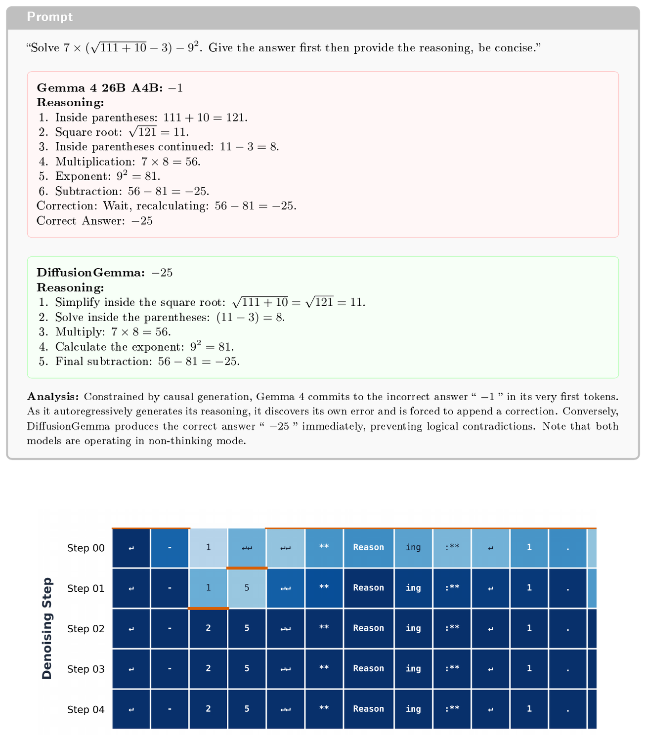
AR next-token prediction is inherently causal; during the generation of a given token, the model can only attend to the preceding context. It fundamentally lacks the capacity to condition upon tokens that have yet to be generated. By contrast, text diffusion operates with full bidirectional attention across the canvas. This non-causal property allows tokens at arbitrary positions across the canvas to attend simultaneously to both past and future representations—a critical capability for complex planning and reasoning tasks where early decisions depend on eventual outcomes (e.g., [134, 135, 136, 137]). Consequently, locally within a canvas, future tokens can directly influence the formation of earlier tokens.
Because text diffusion employs an iterative refinement process, it possesses a built-in mechanism for self-correction. Any premature commitments generated in earlier denoising steps can be revised during subsequent denoising iterations ([138, 139]). While we have previously demonstrated the efficacy of bidirectional reasoning and self-correction in structured logic puzzles like Sudoku, we demonstrate these mechanics in two reasoning examples.
Consider the multi-step arithmetic problem detailed in Figure 15. Constrained by causal generation, the AR Gemma model must commit to the first token of the final answer before articulating the intermediate calculations. This forces an incorrect initial prediction ($-1$) that the model must later correct. DiffusionGemma, conversely, leverages its bidirectional attention canvas to simultaneously evolve the final answer and its underlying logic. As visualized in the accompanying denoising trace, the parallel diffusion process explores incorrect intermediate states but uses the emerging reasoning tokens to course-correct, seamlessly converging on the correct answer ($-25$). See Appendix H.1 for the second example of logical reasoning and correction via bidirectional attention and denoising.
9.2 Dynamic and Adaptive Computation
Unlike AR models, which inherently allocate a fixed amount of computation per generated token, text diffusion facilitates dynamic test-time compute. Text diffusion models can autonomously calibrate the computational effort expended on a given prompt, trading increased inference time for enhanced generative performance based on the inherent difficulty of the task ([140]). DiffusionGemma automatically adapts to task difficult via adaptive stopping. As illustrated in Figure 5, tasks of varying complexity organically elicit different numbers of effective denoising steps. This allows the model to conserve compute on easier queries while expending more compute on complex reasoning. In Appendix H.2 we concretely illustrate the adaptive behavior of text diffusion by contrasting a structurally “hard” generation task against a structurally “easy” task and show that the easy task requires fewer denoising steps, as well as showing how the information propagates differently across the canvas of tokens in these two cases.
Furthermore, the maximum number of denoising steps serves as an explicit configuration parameter to manage the latency-quality tradeoff. A lower step count forces the model to traverse the reverse process more coarsely, yielding faster results with a corresponding reduction in output precision. Expanding the step count allows for a finer resolution during generation, maximizing quality while extending the required compute time. Figure 10 plots this continuous relationship, demonstrating how the model can be dynamically calibrated to suit varied operational constraints.
9.3 Structured and Constrained Outputs
In many practical applications, the desired output adheres to a rigid, highly structured format (e.g., JSON schemas) or exhibits strong lexical dependence on the input prompt, such as in optical character recognition (OCR), code editing tasks, or fine-grained syntactic control ([141, 42]). Because text diffusion generates and refines all tokens in parallel, it seamlessly exploits these structural priors to accelerate convergence. AR models lack this capability; constrained by strict sequential decoding, they must incur the same $O(N)$ computational cost to generate $N$ tokens, even when those tokens consist of rigid boilerplate or verbatim copies of the input context. By contrast, DiffusionGemma can identify and lock in predictable syntactic structures across the entire sequence simultaneously. We highlight this efficiency through two real-world examples: strict JSON extraction (Appendix H.3, Figure 26 and Figure 27) and Python code debugging (Appendix H.3, Figure 28 and Figure 29). Both cases clearly illustrate that the highly constrained output allows the diffusion process to converge in merely two to three steps, drastically reducing latency compared to sequential decoding.
10. Limitations & Known Issues
Section Summary: DiffusionGemma falls short of its autoregressive starting model in overall quality because it was adapted from existing weights with limited fine-tuning and an algorithm tuned for speed rather than peak performance. The model also tends to generate very short answers, occasionally repeats tokens, and sometimes skips required closing tags on multimodal tasks, all side effects of running with very few denoising steps. While it delivers strong speed at low user loads, its higher per-token cost causes it to lose its throughput advantage once dozens of requests run in parallel.
In the previous section, we discussed new emergent properties of text diffusion and advantages of our approach relative to AR language modeling. While DiffusionGemma establishes a new Pareto frontier for generative text modeling and inference efficiency, the current experimental release has these known limitations:
- Performance gap relative to the AR baseline: Lower absolute performance than its AR initialization (Gemma 4 26B A4B) stems from several practical constraints: bypassing native diffusion pretraining to warm-start from AR weights; relying on a comparatively short SFT phase due to compute budget constraints; using an online learning algorithm (SD $\cdot$ RL) that explicitly targets ultra-low latency, intrinsically trading off asymptotic performance; and inheriting architectural, optimization, and data-mixture decisions from the AR baseline that may be suboptimal for the discrete diffusion paradigm.
- Generation length and conciseness: As mentioned in Section 5, our final checkpoint produces highly concise outputs. While this emergent brevity acts as a multiplier for inference speed, it precludes the model from leveraging the quality improvements typically unlocked by longer, more elaborate reasoning traces.
- Occasional token stuttering: In rare instances, the model's output degenerates into repetitive loops or localized stuttering (e.g., endlessly repeating a common token like "the the the"). While our SD $\cdot$ RL training successfully mitigates the vast majority of such instances, this uncommon artifact remains a direct consequence of operating in an ultra-low latency regime, where the aggressively reduced number of denoising steps can occasionally compromise the robustness of the generation process.
- Occasional omission of closing thought tags in multimodal tasks: When processing multimodal prompts, the model does not always reliably generate a closing thought tag (even when the reasoning is correct). This can artificially drag down performance in thinking mode on specific benchmarks; for example, on MMMU-Pro, the thinking score drops below the non-thinking score (54.3 vs. 66.0). This was identified too late in the pipeline to apply a fix for this release.
- Throughput limits at high batch sizes: DiffusionGemma excels at low batch sizes by trading memory-bandwidth costs for compute, outperforming Gemma 4 AR (with MTP) in both per-user and total throughput for up to $\sim$ 32 concurrent users (Figure 12). Beyond this point, the higher per-token compute cost causes AR models to gain a throughput advantage. As noted in Section 6, these results are obtained without targeted batch-size optimization; a thorough empirical analysis under realistic traffic conditions remains future work.
11. Conclusion
Section Summary: DiffusionGemma shows how an existing large language model can be adapted through targeted training to generate text much faster while using fewer computing resources. The resulting system reaches around 1,500 tokens per second on a single high-end GPU and still delivers strong reasoning and multimodal performance, improving the usual trade-off between speed and quality. By releasing the model weights and supporting code openly, the work invites researchers and developers to explore and refine text diffusion methods further.
DiffusionGemma demonstrates a practical, compute-efficient path to ultra-fast text generation. By finetuning the existing Gemma 4 26B A4B AR model to perform text diffusion through our two-stage training pipeline (SFT and SD $\cdot$ RL), it establishes a new Pareto frontier for the speed-to-intelligence tradeoff—achieving around 1, 500 tokens per second on a single H100 while retaining highly competitive reasoning and multimodal capabilities. By releasing DiffusionGemma as an experimental open-weight model—alongside reference implementations in HuggingFace Transformers and vLLM—we aim to empower the open-source community to push the boundaries of text diffusion. We hope researchers and practitioners will build upon this approach, whether by finetuning for specialized tasks, exploring novel sampling algorithms, or further optimizing inference efficiency.
Appendix
Section Summary: The appendix begins by listing all core contributors, additional participants, finetuning team members, project leads, and sponsors involved in the work. It then surveys recent related research on continuous and hybrid diffusion methods for text generation as well as speculative decoding techniques that aim to speed up inference. Finally, it presents before-and-after examples illustrating how an additional reinforcement-learning stage reduces repetitive looping and enables more complete reasoning outputs.
A. Contributions and Acknowledgments (listed alphabetically)
Core contributors (workstream leads marked with ‘*’)
Adrien Ali Taïga James Assiene Daniele Calandriello* Rahma Chaabouni João Gante* Tamara von Glehn* Nate Keating Chris Knutsen Martin Kukla* Tianlin Liu Ivan Lobov* Ofir Nabati João Gabriel Oliveira Nicolas Perez-Nieves* Nastasia Prutianova Bobak Shahriari* Jean Tarbouriech* Pavel Tyletski Çağlar Ünlü Cindy Wu
Contributors
Glenn Cameron Jerome Connor Sertan Girgin Maarten Grootendorst Alon Levkovitch Eliya Nachmani Omar Sanseviero Piotr Stanczyk
Finetuning framework
Quentin Berthet Andrew Campbell Clément Crepy Valentin De Bortoli Arnaud Doucet Romuald Elie Alexandre Galashov Klaus Greff Alexis Jacq David Ruhe Yu-Han Wu
Leads
Sebastian Flennerhag Brendan O'Donoghue George Scrivener Shantanu Thakoor
Acknowledgements
Sander Dieleman
Lucas Dixon
Johan Ferret
Parnian Kassraie
Preethi Lahoti
Gaël Liu
Sarah Perrin
Angéline Pouget
Louis Rouillard
Pier Giuseppe Sessa
Danilla Sinopalnikov
Gemma Team
Sponsors
Olivier Bachem Jeff Dean Zoubin Ghahramani Raia Hadsell Demis Hassabis Prateek Jain Armand Joulin Koray Kavukcuoglu Marc’Aurelio Ranzato Oriol Vinyals
B. Related work
B.1 Continuous Diffusion for Text
While discrete diffusion remains highly effective, recent advances indicate a resurgence of continuous and hybrid approaches. Flow-matching frameworks like Embedded Language Flows have demonstrated that by abandoning per-step token supervision and remaining in an unrestricted continuous embedding space until a final discretization step, continuous models can substantially outperform discrete baselines ([48]). Building on this continuous paradigm, recent advances in flow maps for discrete data have shown that by aligning training dynamics with the geometry of the probability simplex, these generative trajectories can be compressed into single-step mappings, achieving high-quality parallel language generation in one or a few steps ([142, 143]). Similarly, models utilizing pretrained contextual autoencoders (e.g., Cosmos, TEncDM) map text into compressed, smooth latent spaces where Gaussian diffusion operates efficiently without rounding errors, providing a continuous manifold that lends itself well to advanced guidance techniques ([144, 47, 46]), while recent approaches like hyperspherical flows avoid Gaussian corruption by rotating token embeddings on a hypersphere to better match the geometric structure of language ([145]). Other hybrid frameworks, such as CANDI ([146]), address the "temporal dissonance" of applying Gaussian noise to discrete data by decoupling discrete and continuous corruption, allowing the model to simultaneously learn conditional structure and continuous geometry. Concurrently, Score Entropy Discrete Diffusion has bridged these domains by applying continuous-time Markov chains to learn the probability ratios of discrete data distributions ([51]). These breakthroughs suggest that the initial failures of continuous text diffusion may have been artifacts of sub-optimal spatial geometries and restrictive training objectives rather than inherent modality limitations.
B.2 Speculative Decoding
Speculative decoding ([1, 2, 3]) reduces serving latency by utilizing a smaller draft model to propose token sequences that are verified in parallel by a larger target model. The overall latency depends on the generation time of both the draft and target models. AR drafters ([4]) are fundamentally constrained by sequential generation: increasing draft quality requires more parameters, which increases per-token-latency and diminishes end-to-end gains. Parallel drafters such as Medusa ([147]) circumvent this by generating many tokens at once, but do so independently, yielding suboptimal acceptance rates. Diffusion-based drafters recover inter-token dependencies by instead modeling the joint distribution over draft tokens. TiDAR ([148]) uses a single model for diffusion-based drafting, and AR verification—a configuration that DiffusionGemma also supports—while DFlash ([149]) employs a separate model as the drafter. However, it exhibits suffix decay, with acceptance rates declining at later draft positions ([7]). DSpark ([7]) addresses this by adding a lightweight AR module on top of the parallel backbone. In contrast, DiffusionGemma operates as a standalone diffusion model, eliminating the verification bottleneck and scaling to longer generated canvases than draft-then-verify approaches.
C. Samples Before and After texorpdfstringSD $\cdot$ RL Training
To illustrate the impact of our SD $\cdot$ RL phase, Figure 16, Figure 17 contrast representative generations from the SFT model and the final checkpoint. They show how SD $\cdot$ RL training resolves the severe repetitive looping observed in the SFT baseline, allowing the model to complete complex reasoning traces.
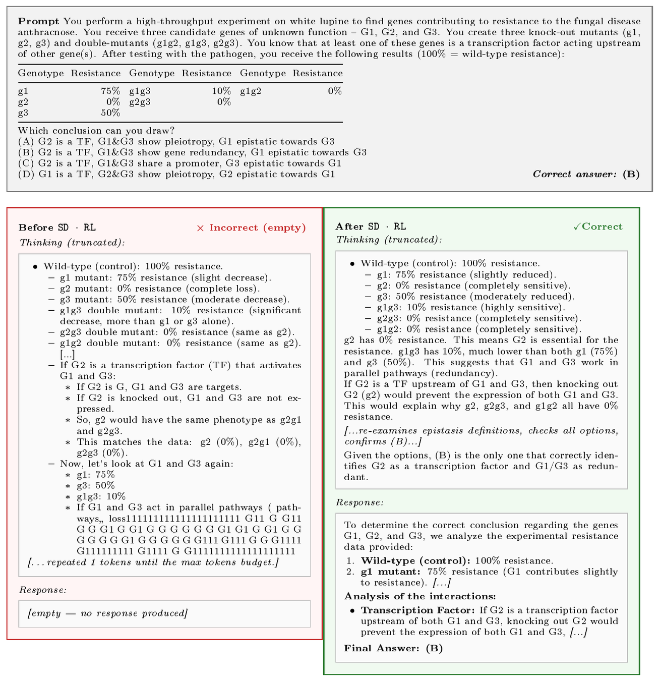

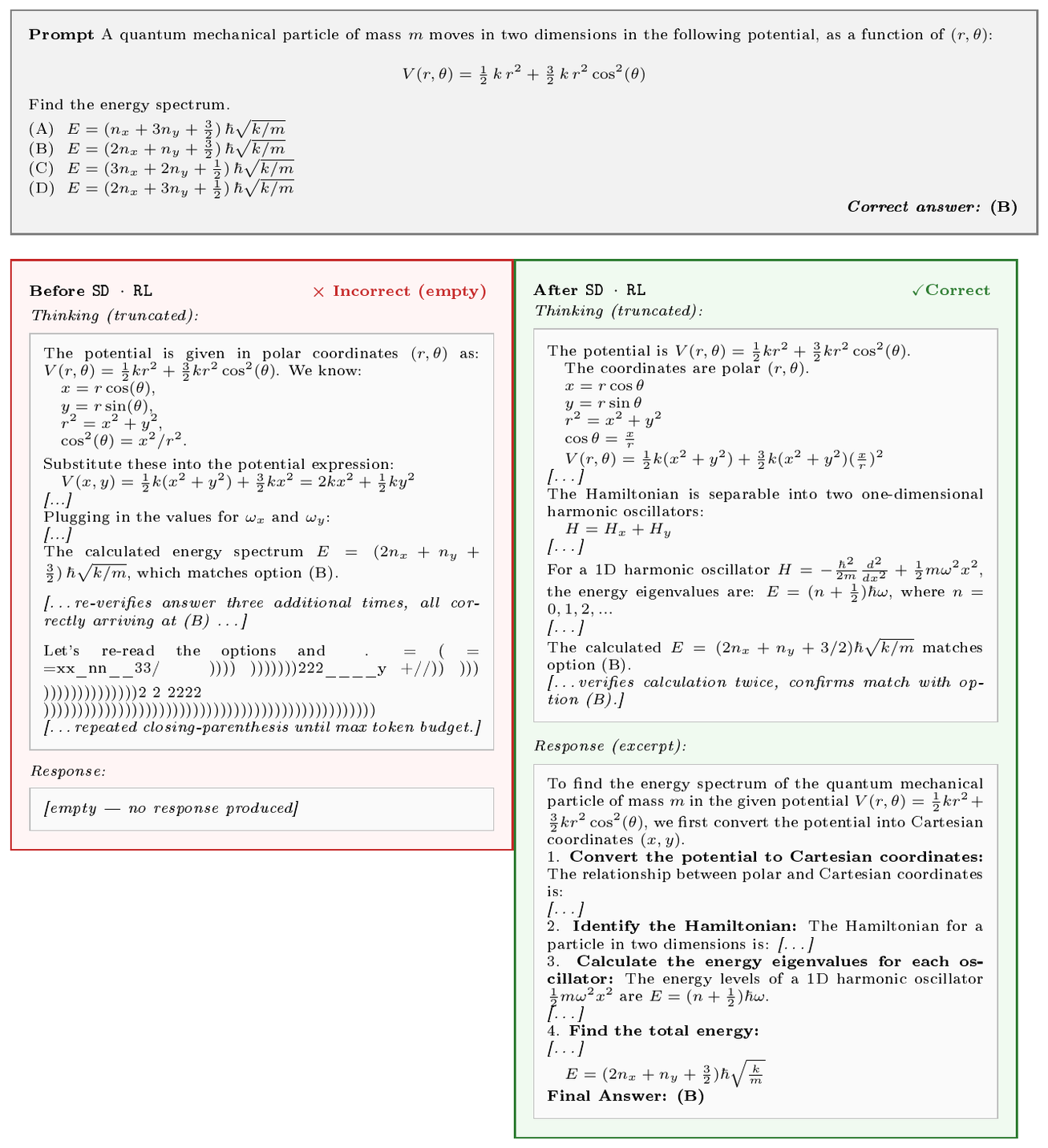
D. Additional Open-Source Downstream Finetuning Results
In Section 8, we describe our finetuning strategy as well as our main results on Sudoku puzzle solving. We now provide full training recipes as well as additional results for PubMedQA ([131]).
Sudoku solving trace summary.
In Figure 18, we present one trace summary for a successful solving of a Sudoku puzzle.
Practical recipe summary.
Table 7 summarizes the key hyperparameters used in Sudoku and PubMedQA. Full training and evaluation code is available open-source via the Hackable Diffusion adapter. For our LoRA strategy to update all the linear layers, using rank 8 for Sudoku solving problem, we only finetune 8M parameters.
Case study: PubMedQA.
To demonstrate applicability beyond structured reasoning, we finetune DiffusionGemma on PubMedQA ([131]), a biomedical question-answering benchmark where the model must read a medical research abstract and produce both a categorical answer (yes, no, or maybe) and a detailed explanatory paragraph. The model is evaluated only on the long task using BLEU score against reference explanations, showing that DiffusionGemma can be effectively adapted to domain-specific natural language generation tasks with minimal data and compute.
: Table 6: PubMedQA performance of the finetuned model with LoRA rank 4. Finetuning leads to a slight increase in accuracy on a model with a good base performance.
| Model | Effective Denoising Steps | Accuracy (%) | BLEU |
|---|---|---|---|
| DiffusionGemma | 18.09 | 75.6 | 10.76 |
| + LoRA finetuning | 31.57 | 76.62 | 20.67 |
\begin{tabular}{lccc}
\toprule
\textbf{Hyperparameter} & \textbf{Sudoku (LoRA)} & \textbf{Sudoku (Full)} & \textbf{PubMedQA} \\
\midrule
LoRA rank & 8 & --- & 4 \\
Canvas size & 256 & 256 & 128 \\
Number of canvases & 1 & 1 & 2 \\
Prompt length & 256 & 256 & 1024 \\
Batch size & 2 & 8 & 2 \\
Peak learning rate & $3 \times 10^{-4}$ & $1.125\times 10^{-4}$ & $1.0 \times 10^{-4}$ \\
End learning rate & $3 \times 10^{-5}$ & $1.125\times 10^{-5}$ & $1.0 \times 10^{-5}$ \\
Training steps & 8{,}000 & 2{,}000 & 2{,}000 \\
Optimizer & Adam & Adafactor & Adam \\
LR schedule & Cosine with warmup & Cosine with warmup & Cosine with warmup \\
Warmup iterations & 400 & 100 & 100 \\
Weight decay & $10^{-4}$ & $10^{-4}$ & $10^{-4}$ \\
Min. hardware & 2 $\times$ A100 80GB & 8 $\times$ A100 80GB & 2 $\times$ A100 80GB \\
\bottomrule
\end{tabular}
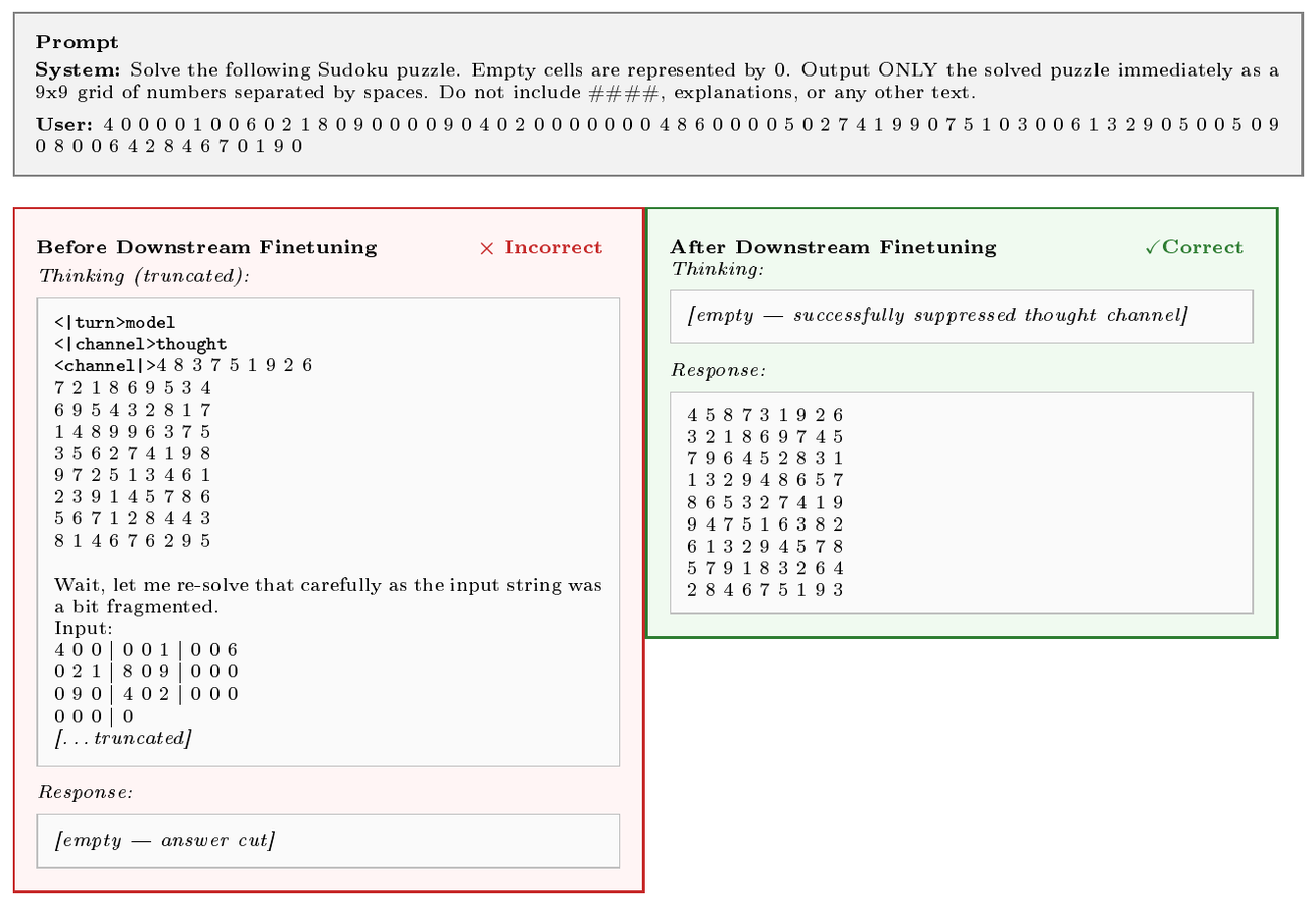
E. Prompt Formatting
To facilitate complex, multi-turn interactions, multimodal inputs, and agentic workflows, the model employs a structured Jinja2-based chat template. This template serializes the conversation history, system instructions, and tool schemas into a standardized string format using specialized control tokens. Explicit formatting ensures the model can accurately distinguish between user inputs, internal reasoning, tool invocations, and system-level contexts. What follows is a summary of the main features, but please refer to the implementation^6 for full details.
E.1 BOS and EOS Special Tokens
As in other Gemma models, every conversation must start with a special BOS token, which has no text rendering but corresponds to token integer 2. The BOS special token must either be manually prepended to the tokenized input or usually by the tokenizer via an add_bos=True keyword argument. At the other end, when a block-AR generation completes, it ends in the usual special token <turn|> followed by padding with the EOS token. Similarly, the EOS token corresponds to the integer 1 but has no text rendering when detokenized.
E.2 Conversational Structuring
The template strictly delineates conversation turns using opening and closing tags. <|turn> and <turn|> tokens encapsulate individual messages, and the opening token is appended with the specific role (e.g., <|turn>system\n). The model expects four roles: system, user, model, and tool for tool call responses.
The template natively supports multimodal routing by parsing content arrays for specific media types, injecting <|image|> tokens into the context stream where appropriate. In the forward pass of the model, these tokens are replaced by the input image features, as opposed to the corresponding token embedding.
E.3 Thinking Channels
As with the Gemma 4 models, DiffusionGemma supports thinking mode, which can be enabled by adding the thinking token <|think|> to the system instruction. When thinking is enabled, the model will emit an internal reasoning channel (which could technically still be empty) followed by the final answer:
<|channel>thought
# DiffusionGemma's internal reasoning goes here.
<channel|>
# DiffusionGemma's final answer goes here
Importantly, even when the <|think|> token is not present in the system instruction, the model will still emit an empty thought channel as follows:
<|channel>thought
<channel|>
[final answer]
For multi-turn conversations, do not include previous hidden thoughts in the conversation history. Only include the final assistant response before the next user turn.
E.4 Tool and Function Calling Serialization
A significant portion of the template is dedicated to parsing and serializing JSON-like tool schemas into a compact, token-efficient format. All JSON-like schemas, e.g. tool definitions or tool responses, rely on the custom delimiter <|"|> (as opposed to a plain ") for clarity.
<|tool>and<tool|>: Used within the system prompt to define available function schemas, including their descriptions, parameters, and required arguments.<|tool_call>and<tool_call|>: Model requests to invoke tools are formatted as<|tool_call>call:function_name{arguments}<tool_call|>.<|tool_response>and<tool_response|>: Results returned from external tools are appended to the context window wrapped by these tokens, allowing the model to seamlessly integrate external data into its subsequent turns.
F. Mercury 2 Speed Estimation
Estimation data.
As Mercury 2 ([150]) is a closed source model, we do not have direct access to generate speed metrics such as TPF and TPS. We take a black-box approach and estimate TPS by querying OpenRouter's API ^7 with the default maximum sequence (input+output) length of 50, 000. We ran two independent rounds of queries — the first on July 9–10, 2026 (with a small number of retries on July 11), the second round between July 25–26, 2026 — and obtained consistent results across both measurements. Each API response includes the following metadata:
- the number of input tokens (prompt tokenization);
- how many prompt tokens were cached (KV-cache hits vs. fresh prefill);
- total output tokens (split into thinking tokens and answer tokens);
- the wall-clock time for the request (including network latencies and other overheads).
Response metadata does not include a breakdown of generation speed. We estimate generate TPS via a least-squares model, detailed below.
Estimation model.
We estimate per-token generation speed by fitting the following model via non-negative least-squares (NNLS):
$ \text{Total Time} = \alpha \cdot \text{effective_prefill_tokens}
- \beta \cdot \text{total_output_tokens} + \gamma,\tag{14} $
where $\text{effective_prefill_tokens} = \text{prompt_tokens} - \text{cached_tokens}$ is the number of tokens requiring fresh computation, $\alpha$ is the per-token prefill time, $\beta$ is the per-token generation time, and $\gamma$ captures constant per-request overhead (network latency, etc.). From the fitted $\beta$, we obtain the generation speed as $1/\beta$ TPS. The non-negativity constraint reflects that processing tokens, generating tokens, and per-request overhead can only add time. In practice, we disable caching across queries.
In order to capture any potential per-task variation in generation speed (e.g. from adaptive computation methods), we fit Equation 14 independently per benchmark, before taking an arithmetic average. Similarly, for open weight models we compute aggregate TPS measurements by first measuring per-task generative speed and then taking the arithmetic average.
Speed estimates.
Our speed measurements for Figure 1 are based on the GPQA-Diamond and LiveCodeBench-v6 datasets. For Mercury 2, we estimate the generative speed per task using the above methodology. Figure 19 shows the corresponding analysis; we obtain a TPS of 452.6 for GPA Diamond and 525.5 TPS for LiveCodeBench-v6, which translates into an average speed of 489 TPS.
Our speed measurements for Table 3 are based on seven benchmarks where we have measurements for all models: AIME 2026, GPQA Diamond, HumanEval, LBPP, LiveCodeBench-v6, MGSM, and Natural2Code. Again, for Mercury 2 we fit our speed estimation model on each task separately first before taking an arithmetic average. Figure 20 and Figure 21 report the corresponding analysis; we obtain average TPS estimates of 600 TPS for high reasoning effort and 547 TPS for medium reasoning effort. We note that some evals (notably HumanEval and Natural2Code) have outliers that generate 50, 000 tokens at extremely high speeds. These give a slightly favorable bias to our generation speed estimates and also explain why high reasoning effort have a higher TPS than medium reasoning effort. These outliers represent corrupted outputs where the model gets stuck in a thinking loop and exhaust the maximum generation length without returning a valid response.
Inception reports $\sim$ 1000 TPS on NVIDIA Blackwell GPUs[^8] while Artificial Analysis[^9] reports a median of $\sim$ 987 TPS on undisclosed hardware. The difference to our estimate can be due to a number of reasons—in particular different hardware, serving optimizations, and/or different datasets used for measurement (this may have a large impact due to adaptive computation). It is worth noting that Artificial Analysis also reports substantial variance. Our estimate reflects the average speed a user would experience via the OpenRouter API.
[^8]: https://www.inceptionlabs.ai/blog/introducing-mercury-2, retrieved July 28, 2026.
[^9]: https://artificialanalysis.ai/models/mercury-2, retrieved July 28, 2026.
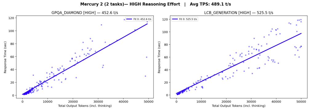
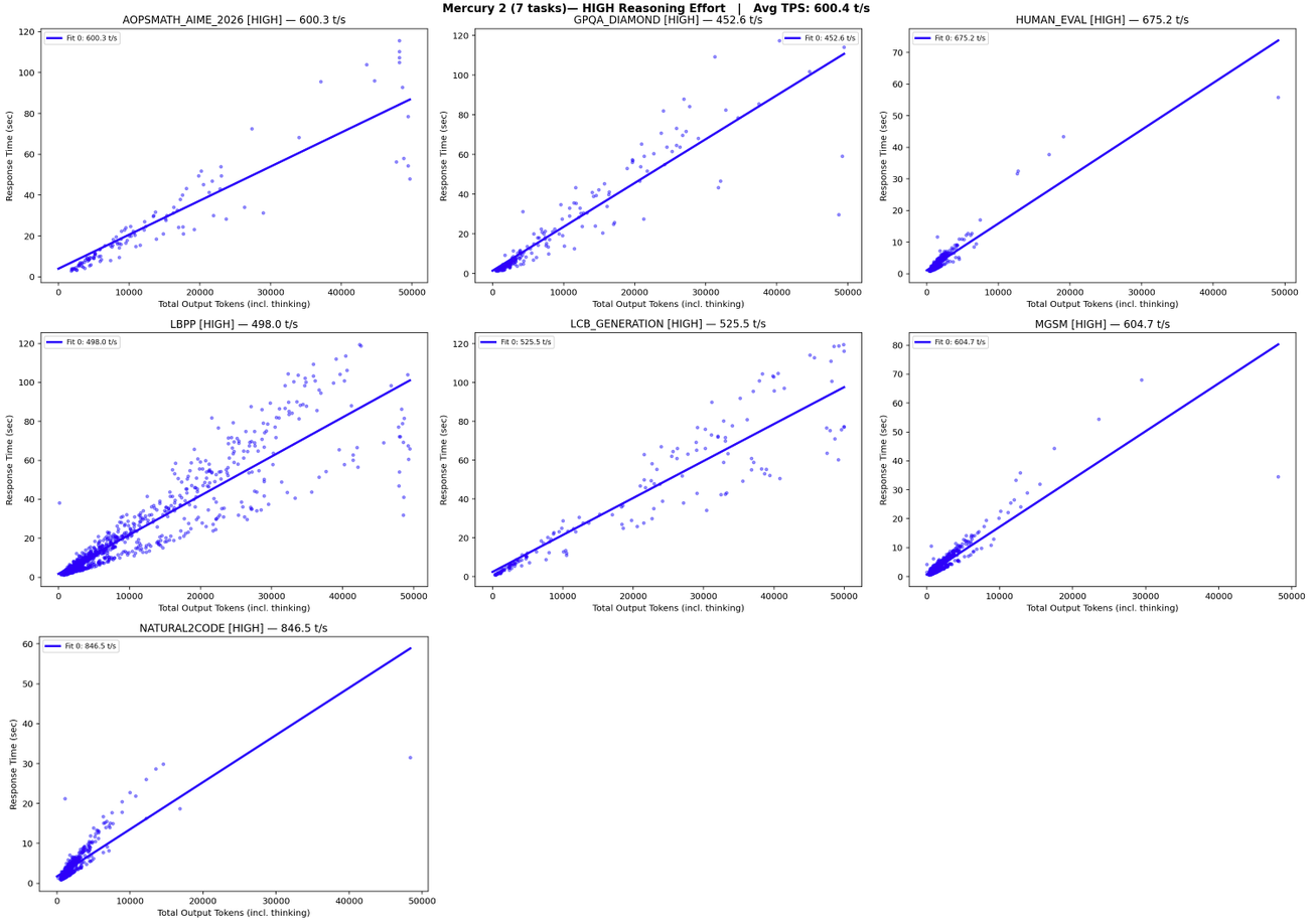
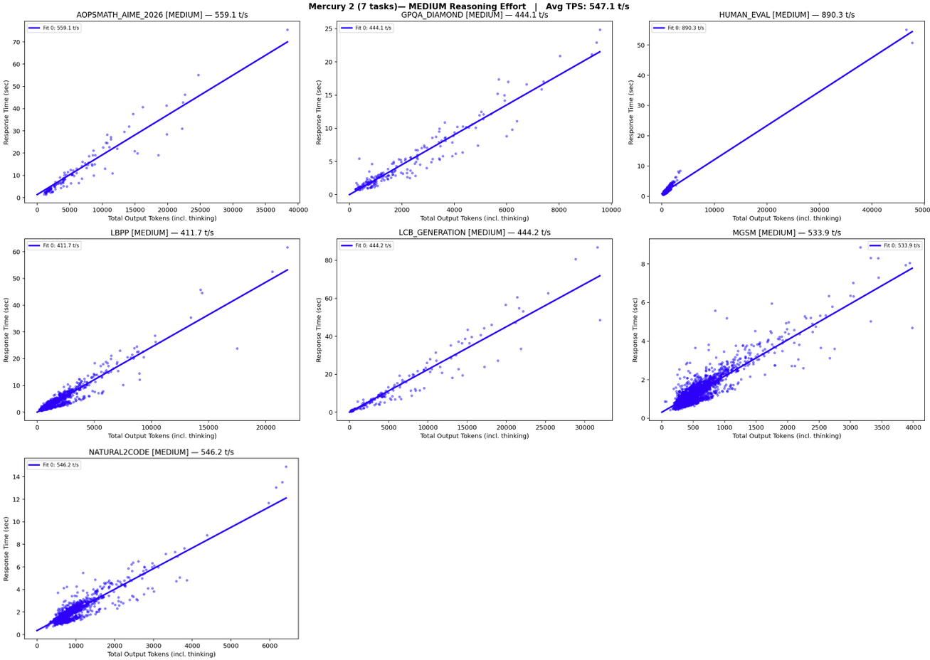
G. Denoising trajectory sampled from DiffusionGemma
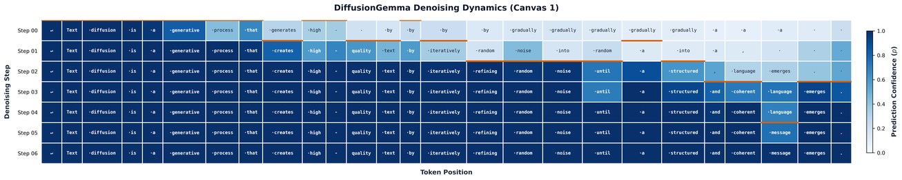
H. More on Practical Advantages of Text Diffusion
H.1 Bidirectional Reasoning and Self-Correction
Consider the frog crossing puzzle in Figure 23. This example highlights the necessity of self-correction in logical deduction. The prompt introduces a deceptive mathematical trap—an infinite loop—that the AR baseline blindly falls into, generating a contradictory "Yes". DiffusionGemma's parallel generation exhibits a distinct self-correction trajectory. While it initially assigns high probability to the intuitive but incorrect "Yes", the bidirectional propagation of the logical constraints across the sequence enables the model to revise its stance and cleanly output "No" before the final tokens are sampled.
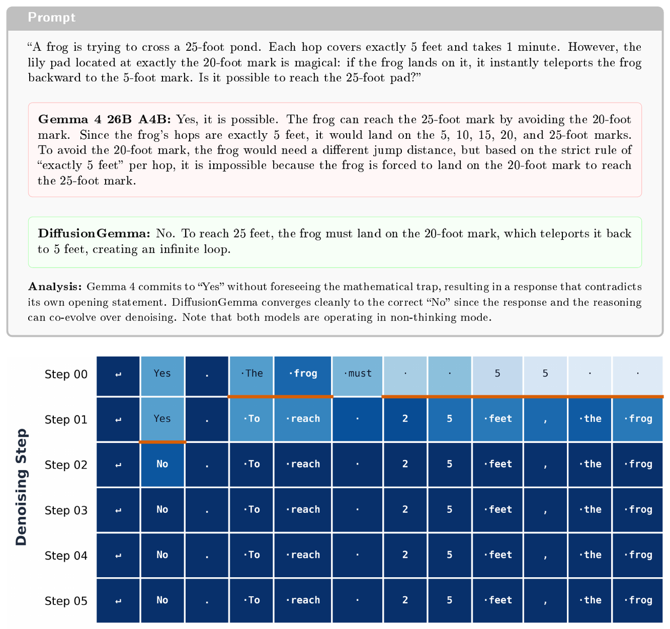
H.2 More on Dynamic and Adaptive Computation
To concretely demonstrate the adaptive behavior of text diffusion, we contrast a structurally "hard" generation task against an "easy" task in Figure 24 and Figure 25. Both tasks involve generating a sequence of binary digits governed by identical local logical rules. However, in the structurally hard variant (Figure 24), each new token strictly depends on the two immediately preceding generated tokens. This causal dependency requires sequential reasoning, forcing the model to resolve the logic in a predominantly left-to-right manner. Consequently, the diffusion process adaptively expends more computational effort, requiring 7 denoising steps to fully resolve the sequence. It is crucial to note, however, that even on this structurally difficult, sequential problem, DiffusionGemma successfully decodes the entire sequence of 40 tokens (20 binary digits and 20 delimiting spaces) in only 7 denoising steps—a substantial acceleration compared to the 40 discrete sequential steps an AR model would require.
Conversely, the "easy" convolutional variant (Figure 25) asks the model to apply the exact same logic rules over a statically provided input string. Because the causal dependency on the model's own dynamic output is removed, the task lacks sequential structure. DiffusionGemma immediately leverages its bidirectional attention to independently resolve all local rules in parallel, allowing the entire output sequence to converge simultaneously in merely 4 denoising steps.
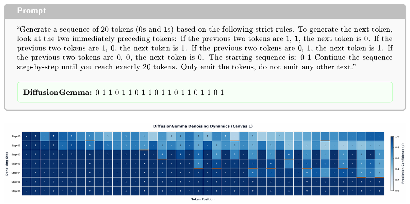
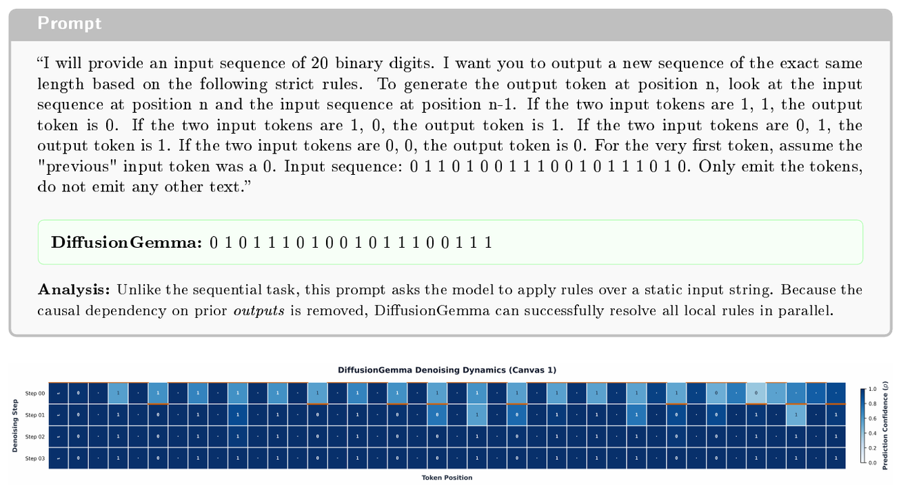
H.3 Structured and Constrained Outputs
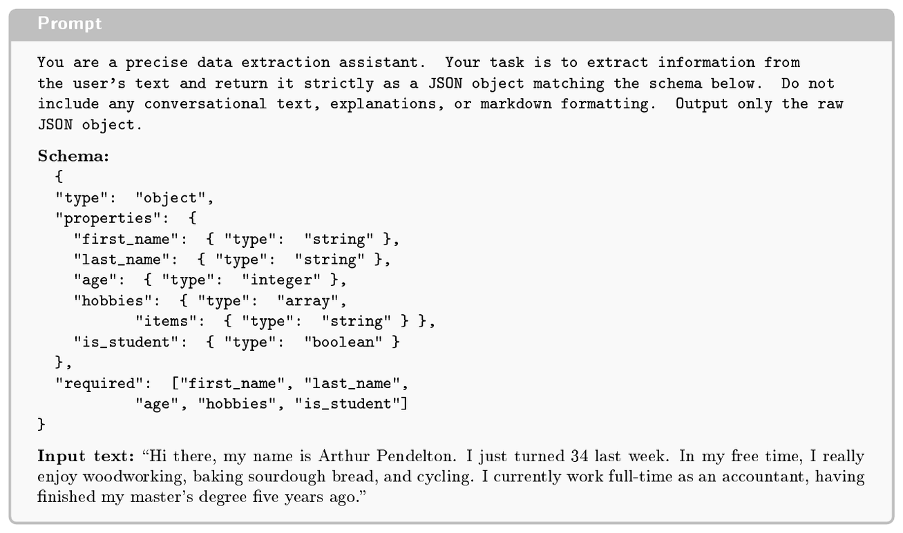
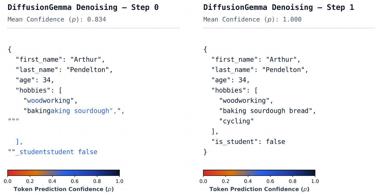
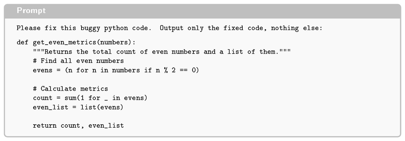
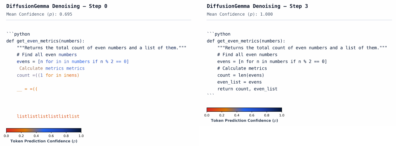
References
Section Summary: The references section lists dozens of academic papers and technical reports focused on accelerating inference in large language models. Many entries describe speculative decoding methods and newer diffusion-based approaches that aim to generate text faster than standard autoregressive techniques, while others trace the development of neural language models, attention mechanisms, and diffusion models from foundational work onward. Together they provide sources on both practical speed-ups for systems like Gemini and broader research into alternative text generation paradigms.
[1] Leviathan et al. (2023). Fast inference from transformers via speculative decoding. In icml.
[2] Chen et al. (2023). Accelerating Large Language Model Decoding with Speculative Sampling. arXiv preprint arXiv:2302.01318.
[3] Xia et al. (2024). Unlocking Efficiency in Large Language Model Inference: A Comprehensive Survey of Speculative Decoding. In Findings of the Association for Computational Linguistics: ACL 2024.
[4] Li et al. (2026). EAGLE-3: Scaling up inference acceleration of large language models via training-time test. In neurips.
[5] Stern et al. (2018). Blockwise Parallel Decoding for Deep Autoregressive Models. In neurips.
[6] Zhao et al. (2024). Lookahead: An Inference Acceleration Framework for Large Language Model with Lossless Generation Accuracy. In Proceedings of the 30th ACM SIGKDD Conference on Knowledge Discovery and Data Mining.
[7] Cheng et al. (2026). DSpark: Confidence-Scheduled Speculative Decoding with Semi-Autoregressive Generation.
[8] Deschenaux, Justin and Gulcehre, Caglar (2024). Promises, Outlooks and Challenges of Diffusion Language Modeling. arXiv preprint arXiv:2406.11473.
[9] Google DeepMind (2025). Gemini Diffusion. https://deepmind.google/models/gemini-diffusion/.
[10] Inception Labs et al. (2025). Mercury: Ultra-Fast Language Models Based on Diffusion. arXiv preprint arXiv:2506.17298.
[11] Nie et al. (2026). Large language diffusion models. In neurips.
[12] Bie et al. (2025). LLaDA 2.0: Scaling up diffusion language models to 100b. arXiv preprint arXiv:2512.15745.
[13] Song et al. (2025). Seed diffusion: A large-scale diffusion language model with high-speed inference. arXiv preprint arXiv:2508.02193.
[14] Yonggan Fu et al. (2026). Nemotron-Labs-Diffusion: A Tri-Mode Language Model Unifying Autoregressive, Diffusion, and Self-Speculation Decoding.
[15] Gemma Team et al. (2026). Gemma 4 technical report. arXiv preprint arXiv:2607.02770.
[16] Google DeepMind (2026). Accelerating Gemma 4: faster inference with multi-token prediction drafters. https://blog.google/innovation-and-ai/technology/developers-tools/multi-token-prediction-gemma-4/.
[17] DeepSeek-AI (2024). DeepSeek-V3 Technical Report. arXiv preprint arXiv:2412.19437.
[18] Unsloth (2026). DiffusionGemma. https://unsloth.ai/docs/models/diffusiongemma. Accessed: 2026-06-11.
[19] Han et al. (2024). Transfer learning for text diffusion models. arXiv preprint arXiv:2401.17181.
[20] Shansan Gong et al. (2025). Scaling Diffusion Language Models via Adaptation from Autoregressive Models. In iclr.
[21] Gemini Team (2025). Gemini 2.5: Pushing the Frontier with Advanced Reasoning, Multimodality, Long Context, and Next Generation Agentic Capabilities. arXiv preprint arXiv:2507.06261.
[22] Interfaze (2026). The First Open Source Diffusion Audio ASR Model. https://interfaze.ai/blog/the-first-open-source-diffusion-audio-asr-model. Blog post.
[23] Van Puyvelde et al. (2026). Discrete Diffusion Language Models for Interactive Radiology Report Drafting. arXiv preprint arXiv:2607.01436.
[24] Bengio et al. (2003). A neural probabilistic language model. Journal of Machine Learning Research. 3. pp. 1137–1155.
[25] Mikolov et al. (2010). Recurrent neural network based language model. In Interspeech.
[26] Graves, Alex (2013). Generating sequences with recurrent neural networks. arXiv preprint arXiv:1308.0850.
[27] Sutskever et al. (2014). Sequence to sequence learning with neural networks. In neurips.
[28] Vaswani et al. (2017). Attention is All you Need. In neurips.
[29] Gu et al. (2018). Non-autoregressive neural machine translation. In iclr.
[30] Nikolay Savinov et al. (2022). Step-unrolled Denoising Autoencoders for Text Generation. In iclr.
[31] Sohl-Dickstein et al. (2015). Deep unsupervised learning using nonequilibrium thermodynamics. In icml.
[32] Ho et al. (2020). Denoising diffusion probabilistic models. In neurips.
[33] Song et al. (2021). Score-Based Generative Modeling through Stochastic Differential Equations. In iclr.
[34] Holderrieth, Peter and Erives, Ezra (2025). An Introduction to Flow Matching and Diffusion Models. arXiv preprint arXiv:2506.02070.
[35] Song, Yang and Ermon, Stefano (2019). Generative Modeling by Estimating Gradients of the Data Distribution. In neurips.
[36] Song et al. (2021). Denoising Diffusion Implicit Models. In iclr.
[37] Song et al. (2021). Maximum Likelihood Training of Score-Based Diffusion Models. In neurips.
[38] Meng et al. (2022). SDEdit: Guided Image Synthesis and Editing with Stochastic Differential Equations. In iclr.
[39] Lipman et al. (2023). Flow Matching for Generative Modeling. In iclr.
[40] De Bortoli et al. (2021). Diffusion Schrödinger Bridge with Applications to Score-Based Generative Modeling. In neurips.
[41] Yi et al. (2024). Diffusion models in text generation: a survey. PeerJ Computer Science.
[42] Li et al. (2022). Diffusion-LM Improves Controllable Text Generation. In neurips.
[43] Strudel et al. (2022). Self-conditioned Embedding Diffusion for Text Generation. arXiv preprint arXiv:2211.04236.
[44] Sander Dieleman et al. (2022). Continuous diffusion for categorical data. arXiv preprint arXiv:2211.15089.
[45] Kingma et al. (2021). Variational Diffusion Models. In neurips.
[46] Shabalin et al. (2025). TEncDM: Understanding the Properties of the Diffusion Model in the Space of Language Model Encodings. In aaai.
[47] Viacheslav Meshchaninov et al. (2025). Cosmos: Compressed and Smooth Latent Space for Text Diffusion Modeling. In neurips.
[48] Hu et al. (2026). ELF: Embedded Language Flows. arXiv preprint arXiv:2605.10938.
[49] Austin et al. (2021). Structured denoising diffusion models in discrete state-spaces. In neurips.
[50] Sahoo et al. (2024). Simple and Effective Masked Diffusion Language Models. In neurips.
[51] Lou et al. (2024). Discrete Diffusion Modeling by Estimating the Ratios of the Data Distribution. In icml.
[52] Lingxiao Zhao et al. (2025). Unified Discrete Diffusion for Categorical Data. Journal of Machine Learning Research. 26(215). pp. 1–49.
[53] Devlin et al. (2019). BERT: Pre-training of deep bidirectional transformers for language understanding. In naacl.
[54] Liu et al. (2019). RoBERTa: A robustly optimized bert pretraining approach. arXiv preprint arXiv:1907.11692.
[55] Sanh et al. (2019). DistilBERT, a distilled version of BERT: smaller, faster, cheaper and lighter. arXiv preprint arXiv:1910.01108.
[56] Kevin Clark et al. (2020). ELECTRA: Pre-training Text Encoders as Discriminators Rather Than Generators. In iclr.
[57] Gat et al. (2024). Discrete flow matching. In neurips.
[58] Campbell et al. (2022). A Continuous Time Framework for Discrete Denoising Models. In neurips.
[59] Campbell et al. (2024). Generative Flows on Discrete State-Spaces: Enabling Multimodal Flows with Applications to Protein Co-Design. In icml.
[60] Hoogeboom et al. (2022). Autoregressive Diffusion Models. In iclr.
[61] Hoogeboom et al. (2021). Argmax flows and multinomial diffusion: Learning categorical distributions. In neurips.
[62] Ou et al. (2025). Your Absorbing Discrete Diffusion Secretly Models the Conditional Distributions of Clean Data. In iclr.
[63] Lewis et al. (2020). BART: Denoising Sequence-to-Sequence Pre-training for Natural Language Generation, Translation, and Comprehension. In acl.
[64] Colin Raffel et al. (2020). Exploring the Limits of Transfer Learning with a Unified Text-to-Text Transformer. Journal of Machine Learning Research.
[65] Wu et al. (2025). FastDLLM v2: Efficient Block-Diffusion LLM. arXiv preprint arXiv:2509.26328.
[66] Arriola et al. (2025). Block Diffusion: Interpolating Between Autoregressive and Diffusion Language Models. In iclr.
[67] Deschenaux, Justin and Gulcehre, Caglar (2026). BlockGen: Flexible Blockwise Sequence Modeling with Hybrid Samplers. In iclr.
[68] Chen et al. (2023). Analog Bits: Generating Discrete Data using Diffusion Models with Self-Conditioning. In iclr.
[69] Jo et al. (2026). Loopholing Discrete Diffusion: Deterministic Bypass of the Sampling Wall. In iclr.
[70] Engels et al. (2026). How Transparent is DiffusionGemma?. arXiv preprint arXiv:2606.20560.
[71] Asaria et al. (2026). Neither Parallel Nor Sequential: How DiffusionGemma Actually Commits Tokens. arXiv preprint arXiv:2606.14620.
[72] Lezama et al. (2023). Predictor-Corrector Sampling for Discrete Diffusion Models. In iclr.
[73] Deschenaux et al. (2026). The Diffusion Duality, Chapter II: $\Psi$-Samplers. In iclr.
[74] Liu et al. (2026). NI Sampling: Accelerating Discrete Diffusion Sampling by Token Order Optimization. In iclr.
[75] Yao et al. (2026). Accelerating Discrete Diffusion Models with Parallel-In-Time Sampling. arXiv preprint arXiv:2607.00773.
[76] Yinuo Ren et al. (2025). Fast Solvers for Discrete Diffusion Models: Theory and Applications of High-Order Algorithms. In neurips.
[77] Ben-Hamu et al. (2026). Accelerated sampling from masked diffusion models via entropy bounded unmasking. In neurips.
[78] Chang et al. (2022). MaskGIT: Masked Generative Image Transformer. In cvpr.
[79] Zhang et al. (2024). EDT: Improving Large Language Models' Generation by Entropy-based Dynamic Temperature Sampling. arXiv preprint arXiv:2403.14541.
[80] Zelikman et al. (2024). Quiet-STaR: Language Models Can Teach Themselves to Think Before Speaking. In colm.
[81] Black et al. (2024). Training diffusion models with reinforcement learning. In iclr.
[82] Liu et al. (2025). Flow-GRPO: Training flow matching models via online RL. In neurips.
[83] Zheng et al. (2026). DiffusionNFT: Online diffusion reinforcement with forward process. In icml.
[84] Zhao et al. (2026). d1: Scaling reasoning in diffusion large language models via reinforcement learning. In neurips.
[85] Ma et al. (2026). Reinforcement learning with discrete diffusion policies for combinatorial action spaces. In icml.
[86] Wallace et al. (2024). Diffusion Model Alignment Using Direct Preference Optimization. In cvpr.
[87] Fan et al. (2023). DPOK: Reinforcement Learning for Fine-tuning Text-to-Image Diffusion Models. In neurips.
[88] Clark et al. (2024). Directly Fine-Tuning Diffusion Models on Differentiable Rewards. In iclr.
[89] Dong et al. (2023). RAFT: Reward rAnked FineTuning for Generative Foundation Model Alignment. Transactions on Machine Learning Research.
[90] Lee et al. (2023). Aligning Text-to-Image Models using Human Feedback. arXiv preprint arXiv:2302.12192.
[91] Tim Salimans and Jonathan Ho (2022). Progressive Distillation for Fast Sampling of Diffusion Models. In iclr.
[92] Song et al. (2023). Consistency models. In icml.
[93] Deschenaux, Justin and Gulcehre, Caglar (2025). Beyond autoregression: Fast LLMs via self-distillation through time. In iclr.
[94] Feiyang Fu et al. (2025). Learnable Sampler Distillation for Discrete Diffusion Models. In neurips.
[95] Luo et al. (2023). Latent Consistency Models: Synthesizing High-Resolution Images with Few-Step Inference. In neurips.
[96] Sauer et al. (2024). Adversarial Diffusion Distillation. In cvpr.
[97] Liu et al. (2024). InstaFlow: One Step is Enough for High-Quality Diffusion-Based Text-to-Image Generation. In iclr.
[98] Yin et al. (2024). One-Step Image Translation with Text-to-Image Models. In cvpr.
[99] Hoogeboom et al. (2026). Beyond Single Tokens: Distilling Discrete Diffusion Models via Discrete MMD. arXiv preprint arXiv:2603.20155. doi:10.48550/arXiv.2603.20155.
[100] Kwon et al. (2023). Efficient Memory Management for Large Language Model Serving with PagedAttention. In Proceedings of the 29th Symposium on Operating Systems Principles (SOSP).
[101] Pope et al. (2023). Efficiently Scaling Transformer Inference. In Proceedings of Machine Learning and Systems (MLSys).
[102] Google DeepMind Team (2026). DiffusionGemma Implementation in HuggingFace Transformers. https://github.com/huggingface/transformers/pull/46540. Pull Request.
[103] The vLLM Team and Google DeepMind Team (2026). DiffusionGemma: The First Diffusion LLM (dLLM) Natively Supported in vLLM. https://vllm.ai/blog/2026-06-10-diffusion-gemma. vLLM Blog. Implementation: https://github.com/vllm-project/vllm/pull/45163.
[104] Rajbhandari et al. (2022). DeepSpeed-MoE: Advancing Mixture-of-Experts Inference and Training to Power Next-Generation AI Scale. In icml.
[105] Huang et al. (2024). Toward Efficient Inference for Mixture of Experts. In neurips.
[106] Jack W. Rae et al. (2020). Compressive Transformers for Long-Range Sequence Modelling. In iclr.
[107] Dao et al. (2022). FlashAttention: Fast and Memory-Efficient Exact Attention with IO-Awareness. In neurips.
[108] Zadouri et al. (2026). FlashAttention-4: Algorithm and Kernel Pipelining Co-Design for Asymmetric Hardware Scaling. In Proceedings of Machine Learning and Systems.
[109] Zhu et al. (2025). NanoFlow: towards optimal large language model serving throughput. In Proceedings of the 19th USENIX Conference on Operating Systems Design and Implementation.
[110] Tang et al. (2024). Quest: Query-Aware Sparsity for Efficient Long-Context LLM Inference. In icml.
[111] Zhu et al. (2025). MegaScale-Infer: Efficient Mixture-of-Experts Model Serving with Disaggregated Expert Parallelism. In Proceedings of the ACM SIGCOMM 2025 Conference.
[112] Jasper Dekoninck et al. (2026). Beyond Benchmarks: MathArena as an Evaluation Platform for Mathematics with LLMs. In 3rd AI for Math Workshop at the International Conference on Machine Learning (ICML). https://openreview.net/forum?id=DmPE4byHuN.
[113] Cobbe et al. (2021). Training verifiers to solve math word problems. arXiv preprint arXiv:2110.14168.
[114] Freda Shi et al. (2023). Language models are multilingual chain-of-thought reasoners. In iclr.
[115] Tsoukalas et al. (2024). PutnamBench: Evaluating neural theorem-provers on the Putnam mathematical competition. In neurips.
[116] Jain et al. (2025). LiveCodeBench: Holistic and contamination free evaluation of large language models for code. In iclr.
[117] Quan et al. (2025). CodeElo: Benchmarking Competition-level Code Generation of LLMs with Human-comparable Elo Ratings. arXiv preprint arXiv:2501.01257.
[118] Chen et al. (2021). Evaluating large language models trained on code. arXiv preprint arXiv:2107.03374.
[119] Terry Yue Zhuo et al. (2025). BigCodeBench: Benchmarking code generation with diverse function calls and complex instructions. In iclr.
[120] Matton et al. (2024). On leakage of code generation evaluation datasets. In emnlp_findings.
[121] David Rein et al. (2024). GPQA: A Graduate-Level Google-Proof Q&A Benchmark. In colm.
[122] Suzgun et al. (2023). Challenging BIG-Bench Tasks and Whether Chain-of-Thought Can Solve Them. In Findings of the Association for Computational Linguistics: ACL 2023.
[123] OpenAI (2024). Multilingual Massive Multitask Language Understanding (MMMLU). https://huggingface.co/datasets/openai/MMMLU.
[124] Wang et al. (2024). MMLU-Pro: A More Robust and Challenging Multi-Task Language Understanding Benchmark. In neurips.
[125] Yue et al. (2025). MMMU-Pro: A more robust multi-discipline multimodal understanding benchmark. In acl.
[126] Zhou et al. (2023). Instruction-following evaluation for large language models. arXiv preprint arXiv:2311.07911.
[127] Yao et al. (2024). $\tau$-bench: A Benchmark for Tool-Agent-User Interaction in Real-World Domains. arXiv preprint arXiv:2406.12045.
[128] Abramovich et al. (2026). SPEED-Bench: A unified and diverse benchmark for speculative decoding. In icml.
[129] Crepy et al. (2026). Hackable Diffusion: A modular toolbox written in Jax to experiment and educate around Diffusion modeling. Sponsors: A. Doucet and R. Elie. https://github.com/google/hackable_diffusion.
[130] Edward J Hu et al. (2022). LoRA: Low-Rank Adaptation of Large Language Models. In iclr.
[131] Jin et al. (2019). PubMedQA: A Dataset for Biomedical Research Question Answering. In emnlp.
[132] Ghazvininejad et al. (2019). Mask-Predict: Parallel Decoding of Conditional Masked Language Models. In emnlp.
[133] Shansan Gong et al. (2023). DiffuSeq: Sequence to Sequence Text Generation with Diffusion Models. In iclr.
[134] Papadopoulos et al. (2024). Arrows of Time for Large Language Models. In icml.
[135] Ouail Kitouni et al. (2024). The Factorization Curse: Which Tokens You Predict Underlie the Reversal Curse and More. In neurips.
[136] Zhang-Li et al. (2024). Reverse that number! Decoding order matters in arithmetic learning. arXiv preprint arXiv:2403.05845.
[137] Nagarajan et al. (2025). Roll the dice & look before you leap: Going beyond the creative limits of next-token prediction. In icml.
[138] Reid et al. (2022). DiffusER: Discrete Diffusion via Edit-Based Reconstruction. In Proceedings of the 2nd Conference of the Asia-Pacific Chapter of the Association for Computational Linguistics and the 12th International Joint Conference on Natural Language Processing (AACL-IJCNLP).
[139] Han et al. (2023). SSD-LM: Semi-autoregressive Simplex-based Diffusion Language Model for Text Generation and Modular Control. In acl.
[140] Jiacheng Ye et al. (2024). Diffusion of Thought: Chain-of-Thought Reasoning in Diffusion Language Models. In neurips.
[141] Chen et al. (2023). TextDiffuser: Diffusion Models as Text Painters. In neurips.
[142] Lee et al. (2026). Flow Map Language Models: One-step Language Modeling via Continuous Denoising. arXiv preprint arXiv:2602.16813.
[143] Potaptchik et al. (2026). Discrete Flow Maps. arXiv preprint arXiv:2604.09784.
[144] He et al. (2024). Manifold Preserving Guided Diffusion. In iclr.
[145] Deschenaux, Justin and Gulcehre, Caglar (2026). Language Modeling with Hyperspherical Flows. arXiv preprint arXiv:2605.11125.
[146] Pynadath et al. (2026). CANDI: Hybrid Discrete-Continuous Diffusion Models. In icml.
[147] Cai et al. (2024). MEDUSA: Simple LLM inference acceleration framework with multiple decoding heads. In icml.
[148] Liu et al. (2026). TiDAR: Think in Diffusion, Talk in Autoregression. In Proceedings of Machine Learning and Systems.
[149] Chen et al. (2026). DFlash: Block Diffusion for Flash Speculative Decoding. In icml.
[150] Inception Labs (2026). Introducing Mercury 2. https://www.inceptionlabs.ai/blog/introducing-mercury-2. Accessed: 2026-07-22.