Correlated initialization of deep residual networks

Felix Benning

Ivan Nourdin

Giovanni Peccati

Abstract

We study the large-depth behavior of residual networks whose weights are correlated across layers at initialization. Our results confirm and extend a conjecture of Marion et al. [2025], according to which correlated initializations should interpolate continuously between the Brownian stochastic differential equation arising from independent initialization and the ordinary differential equation arising from perfectly correlated initialization.

When the initialization is obtained from the application of a feature function to a stationary Gaussian sequence with regularly varying correlation, we prove that there exists a unique critical scaling such that the infinite-depth limit is the solution of a Young differential equation driven by a Hermite process. Hermite processes reduce to the fractional Brownian motion if the feature function generating the initialization has Hermite rank one, which is the case for the identity function, for example. We show that the critical scaling and asymptotic limit are uniquely determined by the decay of correlations together with the Hermite rank of the feature function. Consequently, the correlation structure and Hermite rank of the initialization represent meaningful hyperparameters in the asymptotic regime. By contrast, under finite-variance iid initialization, the asymptotic driver is universally Brownian up to normalization regardless of the choice of distribution.

Our proofs rely on a collection of novel results establishing a robust stability theory for Young differential equations in Banach spaces.

Keywords: Residual networks, correlated initialization, large-depth limit, Young differential equations, Hermite processes, fractional Brownian motion, long-range dependence, functional limit theorems

AMS Classification: 60G18, 60G22, 60H10, 60L20, 60L90, 60F17, 68T07.

Executive Summary: The paper examines the large-depth behavior of residual networks at initialization when weights are correlated across layers. Residual connections made very deep networks trainable, yet the appropriate scaling of residual updates and the resulting dynamics depend strongly on how parameters vary with depth. Independent initialization produces a Brownian-driven stochastic differential equation limit under scaling (L^{-1/2}), while perfectly correlated (smooth) initialization yields an ordinary differential equation limit under scaling (L^{-1}). The work resolves and generalizes the conjecture that intermediate correlations should produce a continuous family of limits between these extremes.

The analysis considers residual networks whose driving increments are obtained by applying a centered feature function of Hermite rank (q) to a stationary Gaussian sequence whose correlations decay regularly with index (\alpha \in (0,1/q)). Under the critical scaling (\lambda_L \asymp L^{-H}/\ell(L)^{q/2}) with (H=1-\alpha q/2), the piecewise-linear interpolations of the hidden states converge in Hölder topology to the unique solution of a Young differential equation driven by a Hermite process of rank (q) and self-similarity parameter (H). When (q=1) the driver reduces to fractional Brownian motion; higher ranks produce non-Gaussian limits such as the Rosenblatt process. The same scaling and limit are obtained for a broad class of nonlinear feature functions, whereas finite-variance i.i.d. initialization always yields a Brownian limit after normalization.

These results rest on new stability and approximation theorems for parameter-dependent Young differential equations in Banach spaces, which establish existence, uniqueness, local Lipschitz continuity with respect to the driver, parameters and initial condition, and convergence of Euler schemes in Hölder topology. The theorems apply directly once the partial-sum process of the correlated increments is shown to converge to the Hermite process.

The findings imply that both the decay rate of correlations and the Hermite rank of the feature function become genuine initialization hyperparameters that determine the infinite-depth dynamics and the required scaling. In contrast to the universal Brownian regime, details of the one-layer distribution now matter asymptotically. This supplies a theoretical basis for designing normalization-free architectures whose large-depth behavior can be tuned continuously between deterministic and stochastic regimes.

Sub-critical scalings produce the identity map at initialization. Super-critical scalings are conjectured to cause explosion, though a rigorous proof remains open. Experiments on MNIST with depth-1000 networks initialized from Cauchy-correlated sequences confirm that accuracy collapses below the predicted critical curve for both Hermite ranks one and two, while performance remains good above it; however, the experiments do not yet identify whether the critical initialization scaling or the maximal-local-update scaling (L^{-1}) is preferable for training.

The analysis applies strictly at initialization and assumes bounded, locally Lipschitz activations together with regularly varying Gaussian correlations. Extension to trained networks and to more general correlation structures requires further work. The mathematical results are unconditional once the stated regularity conditions hold.

1. Introduction

Section Summary: Residual connections enable training of extremely deep neural networks by adding small, shortcut updates to hidden states at each layer, an idea central to modern architectures like Transformers. This paper analyzes how the size of those updates must scale with depth depending on how strongly the layer parameters are correlated: smooth correlations yield ordinary differential equation limits, independent parameters produce stochastic differential equations driven by Brownian motion, and intermediate long-range correlations produce fractional Brownian motion. The authors prove that a broad family of Gaussian correlated initializations converges, under the right scaling, to a Young differential equation limit, confirming and generalizing earlier experimental conjectures.

Residual connections are one of the principal architectural ideas that made very deep neural networks trainable. They have become a standard component of modern architectures, including the Transformer architecture ([1]), which underpins modern large language models. Early work introduced general shortcut paths between successive layers ([2]). [3] popularized the idea of residual networks by showing that simple identity shortcuts enable the training of networks with hundreds or even thousands of layers. They further found that the identity map performed best among several shortcut transformations ([4]). The resulting structure—an identity map perturbed by the residual output—motivated the interpretation of the residual output as the rate of change of the hidden state and the network itself as the numerical approximation of a differential equation ([5, 6, 7]).

In this paper, we consider residual networks (ResNets) of depth $L\in \mathbb{N}$, whose hidden states $h_l$ evolve according to

$ h_{l+1} = h_l + \lambda_L \sigma(w_l, h_l) v_l, \qquad l=0, \dots, L-1.\tag{1} $

Here, $\sigma(w_l, h_l) v_l$ is the residual update produced by the $l$ -th layer with parameters $w_l$ and $v_l$ . The scaling factor $\lambda_L>0$ controls the magnitude of this update and therefore how strongly each layer contributes to the overall transformation of the input.

It is worth noting that the explicit depth-dependent scaling factor $\lambda_L$ was not part of the original ResNet formulation. The residual blocks of [3, 4] instead incorporated batch normalization ([8]) to control the scale of activations and gradients throughout the network. Although batch normalization has proved highly effective, it introduces both theoretical and practical complications: its behavior depends on batch statistics and therefore on the batch size, it treats training and inference differently, and it incurs additional memory and communication costs ([9]). These limitations have motivated normalization-free architectures in which the magnitude of the residual updates is controlled directly through depth-dependent scaling or through an appropriate choice of initialization.

While depth-dependent scaling of order $\lambda_L\asymp L^{-1/2}$ repeatedly appears in this literature (e.g. [10, 11, 12, 13]), it is important to highlight that the appropriate choice of the scaling factor does not only depend on the depth of the network, but also on the dependence structure of the parameters across layers.

At one endpoint, [7] studied ResNets whose parameters at initialization are discretizations of paths that vary smoothly with the layer index, with weight-tied initialization providing the simplest perfectly correlated example. Under the scaling $\lambda_L\asymp L^{-1}$, such networks are Euler discretizations of ordinary differential equations (ODEs). Moreover, [7] show that the smooth dependence of the parameters on the layer index is preserved during training, so that the trained networks also admit an ODE limit.

Building on findings by [13, 14, 15], the work by [16] characterizes the other endpoint of parameters initialized independently across layers. They identified $\lambda_L\asymp L^{-1/2}$ as the critical scaling leading to non-trivial large-depth dynamics and proved that the limiting hidden state is the solution of an Itô stochastic differential equation driven by Brownian motion,

$ d \mathscr{h}_s

\sigma(\mathscr{w}_s, \mathscr{h}_s), d B_s. $

More precisely, scalings larger than $L^{-1/2}$ lead to explosion, whereas scalings smaller than $L^{-1/2}$ suppress the random fluctuations and cause the network to converge to the identity map.

The sharp contrast between the ODE regime, obtained when the weights vary smoothly with the layer index, and the Brownian SDE regime, obtained with independent weights, naturally raises the question of whether intermediate correlation structures can interpolate between these two limits. [16] formulated this conjecture and tested it experimentally by initializing the weights with increments of fractional Brownian motion with Hurst parameter $H\in(\frac12, 1)$ . Their experiments suggested that the transition between explosion and identity occurs at the critical scaling

$ \lambda_L\asymp L^{-H}. $

As explained in the next section, the principal aim of this paper is to provide a rigorous and substantially more general answer to this conjecture, extending it beyond the fractional Brownian setting.

Our contributions

1. Large-depth limits under correlated initialization. Our first contribution (see and below) is a rigorous and more general resolution of the conjecture formulated by [16]. Consider first the Gaussian setting. For each coordinate $i$, suppose that $(v_l^i)_{l\geq 0}$ (where $v_l = (v^1_l, ..., v^p_l)$ is given in Equation 1) is a centered stationary Gaussian sequence with regularly varying covariance

$ \mathsf{E}[v^i_0 v^i_k]=: \rho(k)

k^{-\alpha}\ell(k), \qquad \alpha\in(0, 1), $

where $\ell$ is slowly varying. Setting

$ H

1-\tfrac{\alpha}{2} \in \bigl(\tfrac12, 1\bigr), $

we prove that, under the scaling

$ \lambda_L

\tfrac{L^{-H}}{\ell(L)^{1/2}}, $

the interpolated hidden states converge, as the depth tends to infinity, to the solution of the Young differential equation

$ d \mathscr{h}_s

\sigma(\mathscr{w}_s, \mathscr{h}_s), d B_s^H, $

where $B^H$ is a fractional Brownian motion with Hurst parameter $H$ . Thus, fractional Brownian motion need not be built directly into the initialization through its increments, as in the experiments of [16]: it arises naturally as the scaling limit of a broad class of long-range correlated Gaussian initializations.

Our main theorem actually covers the more general case in which each coordinate of $v_l$ is obtained by applying a centered nonlinear function of Hermite rank $q$ (see Equation 4 and the subsequent discussion) to the underlying Gaussian sequence. Provided $\alpha q<1$, the self-similarity parameter and the corresponding scaling become

$ H

1-\tfrac{\alpha q}{2}, \qquad \lambda_L

\tfrac{L^{-H}}{\ell(L)^{q/2}}. $

Under this scaling, the piecewise-linear interpolation of the hidden layers converges in distribution, in Hölder topology, to the unique solution of the Young differential equation

$ d \mathscr{h}_s

\sigma(\mathscr{w}_s, \mathscr{h}_s), d \mathscr{z}^{q, H}_s, \qquad \mathscr{h}_0=Ax, $

where $\mathscr{z}^{q, H}$ is a Hermite process of rank $q$ and self-similarity parameter $H$ ; see Definition 7. Fractional Brownian motion is recovered when $q=1$, while the case $q=2$ corresponds to the so-called Rosenblatt process, as discussed, e.g., by [17, 18] and [19]. We observe that Hermite ranks one and two are especially relevant in applications: the identity map and many transformations used to generate the initialization have Hermite rank one, whereas symmetry may force the first Hermite coefficient to vanish and lead to Hermite rank two ([20]); in general, it is not difficult to construct functions with arbitrarily high Hermite rank. the theorem and therefore identifies a whole family of large-depth limits and shows that both the appropriate scaling and the limiting dynamics are determined jointly by the decay of correlations and the Hermite rank of the initialization.

Our limiting theory contributes towards an asymptotic theory for selecting initialization hyperparameters, namely the one-layer distribution of the weights, their dependence structure across layers, and the depth-dependent scaling factor. Consistently with the central limit theorem, [16] show that independent initialization exhibits a strong universality phenomenon: after centering and normalization, a broad class of finite-variance distributions leads to the same Brownian-driven SDE in the large-depth limit, under the scaling $\lambda_L\asymp L^{-1/2}$. In this regime, many details of the one-layer distribution are therefore asymptotically immaterial. Our main result, the theorem and, shows that the picture changes in the presence of long-range dependence: the decay of correlations and the Hermite rank of the transformation used to generate the weights jointly determine both the appropriate depth scaling and the nature of the limiting driver. Thus, once correlations across layers are introduced, not only their strength and decay, but also the way in which the one-dimensional weight distribution is generated, become relevant initialization hyperparameters. Our results do not provide a complete selection procedure, but they identify which features of the initialization can genuinely alter the infinite-depth dynamics.

Our results also substantially extend the work of [21], who introduced fractional-Brownian-driven neural differential equations to model long-range dependence in a time-series setting: whereas fractional Brownian motion is postulated there as the driving noise, in our setting it arises naturally as a large-depth limit of correlated ResNet initialization, and is further replaced by general Hermite processes for nonlinear transformations of the underlying Gaussian sequence. 2. Stability and approximation of Young differential equations. To prove the ResNet convergence result, we develop a general stability and approximation theory for parameter-dependent Young differential equations in Banach spaces of the form

$ dx_t=\sigma(t, w_t, x_t), dg_t, $

where both the driving signal $g$ and the parameter path $w$ are Hölder continuous with Hölder exponents strictly larger than $1/2$. We establish existence and uniqueness, local Lipschitz continuity of the solution with respect to the initial condition, the driving signal, and the parameter path, as well as convergence of Euler approximations in Hölder topology. The ResNet convergence theorem (the theorem and) then follows as a direct application of these continuity and approximation results, developed in Section 4. This theory is of independent interest beyond the neural-network application.

########## {caption="Remark: Related work on Young differential equations"}

Differential equations driven by paths of finite $p$-variation, with $p<2$, go back to the foundational work of [22] and [23].

Existence, uniqueness, continuity, flow properties, and Euler approximation for autonomous Young differential equations have been studied in several works; see, in particular, ([24, 25]). Time-dependent Young differential equations, including equations driven by fractional Brownian motion, were considered in ([26, 27]). More broadly, Young differential equations fit within the rough-path framework; see, for instance, ([28, 29]) and the systematic presentation in ([30], Chapter 8). Our results extend this literature by treating Banach-space-valued equations with a separate Hölder parameter path and by providing stability and Euler convergence directly in Hölder topology, complementing the classical approximation results for Young and rough differential equations ([31, 32, 25]).

2. Depth Limit with correlated weights at initialization

Section Summary: This section examines the behavior of very deep residual networks when initial weights are correlated across layers instead of chosen independently. It introduces a generalized ResNet formulation and a correlation model based on stationary Gaussian sequences passed through a feature function, showing that the accumulated residual updates converge to a fractional Brownian motion or, more generally, a Hermite process. Under standard assumptions on the activation, the network's internal states then converge to the solution of a differential equation driven by this random process.

In this section, we characterize the large-depth limit of ResNets whose weights are correlated across layers at initialization. After introducing a generalized ResNet architecture, we specify a class of correlated initializations for which the partial sums of residual updates converge to a Hermite process. We then show that, under suitable regularity assumptions on the activation function and the remaining weights, the interpolated hidden states converge to the solution of a Young differential equation driven by this process. The proof combines a functional limit theorem for correlated random walks ([33]) with stability of Young differential equations and convergence of their Euler discretizations (Section 4).

########## {caption="Definition 1: General ResNet"}

A generalized residual network $F= F_{A, B, (v_l){l=0}^{L-1}, (w_l){l=0}^{L-1}}$ with parameters $(A, B, (v_l){l=0}^{L-1}, (w_l){l=0}^{L-1})$ maps an input $x\in \mathbb{R}^{{d_in}}$ through a series of hidden layers

$ \begin{aligned} h_0 &\coloneq A x \ h_{l +1} &\coloneq h_l + \lambda_L \sigma(w_l, h_l) v_l && l \in { 0, \dots, L -1} \end{aligned} $

to an output $F(x) \coloneq B h_{L} \in \mathbb{R}^{{d_out}}$, with

• $\lambda_L\in [0, \infty)$, a scaling factor that depends on the depth $L$ of the ResNet,
• input and output processing matrices $A\in \mathbb{R}^{d\times {d_in}}$ and $B\in \mathbb{R}^{{d_out}\times d}$,
• parameters $w_l\in\mathcal{W}$, where $\mathcal{W}$ is a fixed Banach space, and $v_l\in \mathbb{R}^r$, which determine the residual update through the continuous map

$ \sigma\colon \mathcal{W}\times \mathbb{R}^d \longrightarrow \mathbb{R}^{d\times r}. $

########## {caption="Example: Classic ResNet"}

Classically, a ResNet is of the form

$ h_{l+1} = h_l + \lambda_L V_l \varphi(W_l h_l + b_l), $

with activation function $\varphi\colon \mathbb{R}\to \mathbb{R}$ applied component-wise and parameter matrices $W_l\in \mathbb{R}^{m \times d}$ and $V_l\in \mathbb{R}^{d \times m}$ and a bias vector $b_l$ . This is a special case of the general ResNet (Definition 1) with

$ V_l \varphi(W_l h_l + b_l) = \underbrace{(\varphi(W_l h_l + b_l)^T \otimes \mathbb{I}{d})}{ \displaystyle\eqcolon \sigma(\underbrace{(W_l, b_l)}{\eqcolon w_l}, h_l) } \underbrace{\mathrm{vec}(V_l)}{\displaystyle\eqcolon v_l \mathrlap{\in \mathbb{R}^{m d}}} = \sigma(w_l, h_l) v_l, $

where $vec(A)$ stacks the columns of the matrix $A$ into a vector and $\otimes$ is the Kronecker product (see e.g. [34] Prop. 2).

We now specify the model for correlations between the parameters $v_l$ across layers. For each coordinate, we obtain $v_l$ by applying a feature function to a stationary Gaussian sequence with regularly varying covariance. The construction is most transparent for the identity feature function, in which case $v_l$ is itself a stationary Gaussian sequence. Allowing more general feature functions can yield examples of ResNets whose scaling limits are solutions of stochastic differential equations driven by Hermite processes instead of the fractional Brownian motion.

########## {caption="Definition 2: Correlated initialization"}

For a feature function $\phi \colon \mathbb{R} \to \mathbb{R}$ we define

$ v_l^i \coloneq \phi(\xi_l^i), \qquad i\in { 1, \dots, r}, l \in { 0, \dots, L -1}, $

where $(\xi_l^{i})_{l \in \mathbb{N}_0}$ are stationary Gaussian sequences in $\mathbb{R}$, independent over $i$, with zero mean $\mathsf{E}[\xi_k^i] = 0$, unit variance $\operatorname{Var}(\xi_k^i) = 1$ and regularly-varying correlation of index $\alpha \in (0, 1)$

$ \rho(k) \coloneq \mathsf{E}[\xi_l^i \xi_{l+k}^i] = k^{-\alpha}\ell(k), \quad k\geq 1, l\geq 0, $

where $\ell$ is a slowly varying function.

########## {caption="Remark 3"}

The centering condition

$ \mathsf{E}[v_l^i] = \mathsf{E}[\phi(\xi_l^{i})] = 0\tag{2} $

is essential to obtain an intermediate scaling. If the mean were nonzero, its contribution would accumulate over the $L$ layers and require the scaling $L^{-1}$ . This scaling would average out the random fluctuations and the deterministic mean would dominate the limit. Observe that, for the identity feature function $\phi(x)=x$, the centering condition Equation 2 follows directly from the assumption $\mathsf{E}[\xi_l^i] = 0$ .

Let us first retain the assumption $\phi(x)=x$ . The linearly interpolated partial sums of the correlated initializations then form the interpolated correlated Gaussian random walk

$ \overline{z}s^L \coloneq \lambda_L \Bigl(\sum{l=0}^{\lfloor L s\rfloor -1} v_l + \underbrace{ (L s-\lfloor L s\rfloor)v_{\lfloor L s\rfloor } }_{\text{linear interpolation}} \Bigr), \qquad s\in [0, 1].\tag{3} $

For

$ H=1-\tfrac{\alpha}{2}, \qquad \lambda_L

\tfrac{L^{-H}}{\ell(L)^{1/2}}, $

this process converges in Hölder topology to a fractional Brownian motion with Hurst parameter $H$ ([33]). Thus, the identity case,

$ \phi(x)=x \qquad\text{leads to}\qquad \overline{z}^L\overset{d}\to B^H, $

where $\overset{d}\to$ indicates convergence in distribution in an appropriate topology. This is the correlated analogue of the independent Gaussian setting, where the initialization variables can be viewed as increments of a Brownian motion, which then drives the infinite-depth limit.

To determine what replaces fractional Brownian motion for more general feature functions, we use the Hermite rank of $\phi$ . If $\phi(\xi_l^i)=v_l^i\in L^2(\Omega)$, then $\phi$ admits an expansion in the Hermite polynomials $(H_k)_{k\geq 0}$ (see e.g. ([35], Chapter 1)),

$ \phi(x)

\sum_{k= q}^{\infty}c_kH_k(x), \qquad c_{q}\neq0, \qquad \sum_{k= q}^\infty k! c_k^2<\infty.\tag{4} $

The Hermite rank $q$ of $\phi$ is therefore the smallest index corresponding to a non-zero coefficient in this expansion. Note that the centering assumption $\mathsf{E}[\phi(\xi_l^i)]=0$ in Equation 2 is equivalent to $q\geq1$ . Since $H_1(x)=x$, the identity feature has Hermite rank one, as do many commonly occurring functions ([20]).

For a feature function of generic Hermite rank $q$, provided $\alpha q<1$, the correlated random walk requires a different normalization and has, in general, a non-Gaussian limit. More precisely, setting

$ H

1-\tfrac{\alpha q}{2}, \qquad \lambda_L

\tfrac{L^{-H}} {\ell(L)^{q/2}}, $

the process $\overline{z}^L$ converges in Hölder topology to a Hermite process $(\mathscr{z}^{q, H}s){s\in[0, 1]}$ of rank $q$ and self-similarity parameter $H$ (see Definition 7, as well as ([17], Chapter 3), ([18], Chapter 2) and ([33])). In other words,

$ \text{Hermite rank of } \phi= q \qquad\text{leads to}\qquad \overline{z}^L\overset{d}\to \mathscr{z}^{q, H}. $

The Hermite process of rank $q=1$ is the fractional Brownian motion.

The significance of this functional limit for the ResNet is that $\overline{z}^L$ plays the role of the cumulative driving signal in the residual recursion. Once the remaining parameters $w_l$ are shown to approximate a sufficiently regular path $\mathscr{w}$, the stability results developed below will allow us to pass to the limit in this recursion and prove that the interpolated hidden states converge to the solution of a Young-type differential equation (see Remark 9 for details)

$ d \mathscr{h}_s

\sigma(\mathscr{w}_s, \mathscr{h}_s), d \mathscr{z}^{q, H}_s, \qquad \mathscr{h}_0=Ax. $

We therefore consider the piecewise-linear interpolation of the remaining parameters,

$ \overline{w}_s^L

w_{\lfloor L s\rfloor } + \underbrace{ (L s-\lfloor L s\rfloor) \bigl(w_{\lfloor L s\rfloor +1}

w_{\lfloor L s\rfloor } \bigr) }_{\text{linear interpolation}} $

and assume that $\overline{w}^L$ converges in distribution, in Hölder topology, to some $\mathscr{w}$ as $L\to\infty$ . The overall mechanism can therefore be summarized as

$ \overline{z}^L\overset{d}\to \mathscr{z}^{q, H}, \qquad \overline{w}^L\overset{d}\to \mathscr{w} \qquad\text{implies}\qquad \overline{h}^L\overset{d}\to \mathscr{h}, $

where the written implication follows from the stability of the Young differential equation. We observe that two families of parameters play distinct roles: the variables $v_l$ represent increments of the limiting driver $\mathscr{z}^{q, H}$, whereas the parameters $w_l$ approximate the values $\mathscr{w}_{l/L}$ of the limiting parameter path.

Next we state the required regularity assumptions about the activation function $\sigma$ for our main result. See Remark 18 for a discussion of the technical role played by the boundedness of $\sigma$ in our proofs.

########## {caption="Assumption 4: Regularity of the activation function"}

The function $\sigma\colon \mathcal{W} \times \mathbb{R}^d \to \mathbb{R}^{d \times r}$ is bounded, $| \sigma| _\infty < \infty$, and locally Lipschitz continuous with locally Lipschitz continuous derivatives in the second variable. That is, there exists a continuous function $c\colon \mathbb{R}^2 \to [0, \infty)$ such that

$ \begin{aligned} |\sigma(w, h) - \sigma(\tilde{w}, \tilde{h})| &\le c(|w|, |\tilde{w}|)\Bigl(|h-\tilde{h}| + (1+|h|+|\tilde{h}|)|w-\tilde{w}|\Bigr) \ |\nabla_h \sigma(w, h) - \nabla_h \sigma(\tilde{w}, \tilde{h})| &\le \underbrace{c(|w|, |\tilde{w}|)}{\text{locally bounded}}\underbrace{\Bigl(|h-\tilde{h}| + (1+|h|+|\tilde{h}|)|w-\tilde{w}|\Bigr)}{\text{local Lipschitz control}} \end{aligned} $

The assumption above is sufficient if $w_{\lfloor L s\rfloor } = \mathscr{w}s$ for a fixed Hölder continuous process $\mathscr{w}$ . If we want $w{\lfloor L s\rfloor } = \overline{w}^L_s$ with $\overline{w}^L \overset{d}\to \mathscr{w}$ in Hölder space, then we need the following additional regularity assumption.

########## {caption="Assumption 5: Additional regularity"}

The activation function is differentiable in the first variable, with a gradient that is also locally Lipschitz. More precisely, there exists a continuous function $\tilde{c} \colon \mathbb{R}^4 \to [0, \infty)$ such that

$ |\nabla_w \sigma(w, x) - \nabla_w \sigma(\tilde{w}, \tilde{x})| \le \tilde{c}(|w|, |\tilde{w}|, |x|, |\tilde{x}|)\bigl(|x-\tilde{x}| + |w-\tilde{w}|\bigr). $

########## {caption="Example 6: Sufficiently nice activation function"}

If $\psi \colon \mathbb{R} \to \mathbb{R}$ is a continuously differentiable activation function such that $\psi$ and $\psi'$ are bounded and $\psi'$ is Lipschitz continuous (e.g. $\psi''$ is bounded), then the generalized activation function

$ \sigma(w, x) \coloneq \psi(Wx + b)^T \otimes \mathbb{I}_d \qquad w=(W, b) \in \mathbb{R}^{m\times d} \times \mathbb{R}^m, x\in \mathbb{R}^d $

satisfies Assumption 4 and Assumption 5. Examples for such an activation function $\psi$ are sigmoid functions such as

$ \psi(x) \in \bigl{ \tanh(x), \arctan(x), \tfrac1{1+e^{-x}}, \mathrm{erf}(x) \bigr} . $

Before stating our main result, the theorem and, we formally introduce Hermite processes in Definition 7 and Remark 8, and briefly recall the notion of a Young differential equation in Remark 9.

########## {caption="Definition 7: Hermite process; see e.g. ([17], Def. 3.1)"}

The rank $q$ Hermite process with Hurst index $H \in (\frac12, 1)$ is defined as

$ Z^{q, H}t \coloneq A{q, H} \int_{\mathbb{R}^q}' \int_0^t \prod_{j=1}^q (s-x_j)_+^{-(\frac12 + \frac{1-H}{q})} ds, W(dx_1)\cdots W(dx_q), \quad t\geq 0, $

where $W$ is the Wiener Gaussian white noise measure and $\int'{\mathbb{R}^q} (...) W(dx_1)\cdots W(dx_q)$ indicates a multiple Wiener-Itô integral of order $q$ (see ([35], Section 2.7)). The normalizing constant $A{q, H}$ is selected so that $\mathsf{E}[(Z^{q, H}_1)^2] = 1$ and is known explicitly ([17], Proposition 3.1). Equivalent representations are given e.g. in ([17], Section 3.1.2) and ([19], Cor. 4.2.11).

########## {caption="Remark 8"}

The following facts are well-known (see e.g. ([17], Section 3.1.1)):

• (i) for every $H\in (\frac12, 1)$ and $q\geq 1$, the process $Z^{q, H}$ is $H$-self-similar, that is: for every $c>0$, $(Z_{ct}^{q, H}){t\geq 0}$ and $(c^HZ_t^{q, H}){t\geq 0}$ have the same law;
• (ii) For every $q\geq 1$, $Z^{q, H}$ is centered, has stationary increments and its covariance is given by

$ \mathsf{E}[Z_t^{q, H}Z_s^{q, H}] = \frac12\left{ t^{2H}+s^{2H}- |t-s|^{2H}\right}, \quad s, t\geq 0;\tag{5} $

• (iii) For every $\gamma\in (0, H)$, the process $Z^{q, H}$ admits a modification whose sample paths are locally $\gamma$-Hölder continuous with probability one.

It can be shown that if $q=1$ then, $Z^{1, H}= B^H$ is a standard fractional Brownian motion with Hurst index $H$ (that is, $Z^{1, H}$ is a centered Gaussian process with covariance Equation 5). The Hermite process with rank $q=2$ corresponds to the so-called Rosenblatt process (see e.g. ([17], Section 3.2) or ([18], Section 2.3.2)).

########## {caption="Remark 9: Young Differential Equations"}

In this paper, an equation of the form

$ d h_s= \sigma(w_s, h_s), d z_s, \qquad h_0=a, $

where $z$ is typically a Hermite process, is understood pathwise in the Young sense. More precisely, a stochastic process $h$ is a solution if, for almost every realization of $(w, z)$,

$ h_t

a+\int_0^t \sigma(w_s, h_s), d z_s, \qquad t\in[0, 1]. $

Here, the integral is the Young integral: if $z$ is $\beta$ -Hölder continuous and $s\mapsto \sigma(w_s, h_s)$ is $\eta$ -Hölder continuous, with $\eta, \beta\in (0, 1]$ and $\eta+\beta>1$, then

$ \int_0^t \sigma(w_s, h_s), d z_s

\lim_{\lvert\pi\rvert\to0} \sum_{[u, v]\in\pi} \sigma(w_u, h_u)\bigl(z_v-z_u\bigr), $

where $\pi$ ranges over partitions of $[0, t]$ and $\lvert\pi\rvert$ denotes their mesh. In particular, the integral and the resulting differential equation are defined pathwise, rather than in the Itô sense. Since a Hermite process with self-similarity parameter $H>\frac12$ has sample paths that are $\gamma$ -Hölder continuous for every $\gamma<H$ (see Remark 8), the limiting drivers considered below fall within the Young framework. We refer to [30], Chapter 8 for further details.

The (standard) functional spaces appearing in the following theorem are formally introduced in Definition 13.

########## {caption="Theorem 10: Large depth limit of ResNets with correlated weights at initialization"}

Let $F = F_{A, B, (v_l){l=0}^{L-1}, (w_l){l=0}^{L-1}}$ be a ResNet as in Definition 1 with an activation function $\sigma$ that satisfies Assumption 4 and correlated initialization of $v_l$ as in Definition 2. Let $(w_l){l=0}^{L-1}$ be initialized, independently of $(v_l){l=0}^{L-1}$, with either

Assume that $v_l^i \in L^p(\Omega)$ for some $p > \frac{2}{1-\alpha q}$ and $\alpha \in (0, \frac1 q)$, where $q\ge 1$ is the Hermite rank of the feature function $\phi$ that produces $v_l^i$ .

Then for the scaling

$ \lambda_L = \tfrac{L^{-H}}{\ell(L)^{\frac{q}2}}, $

we have for all $\beta \in (0, \min{ H - \frac1p, \beta_w})$ with $H = 1 - \frac{\alpha q}{2}\in(\frac12, 1)$ that

$ \overline{z}^L \overset{d}\to \mathscr{z}^{q, H}, \text{ in } C^\beta([0, 1], \mathbb{R}^r), \quad\text{and}\quad \overline{h}^L \overset{d}\to \mathscr{h}, \quad \text{in } C^\beta([0, 1], \mathbb{R}^d), \quad \text{as} \quad L \to \infty, $

where

• $\overline{z}^L$ is the interpolated sum process of the parameters $v_l$ defined in Equation 3,
• $\mathscr{z}^{q, H}=\gamma (Z^{q, H, 1}, \ldots, Z^{q, H, r})$ are independent Hermite processes (Def. Definition 7) $Z^{q, H, i}$ of rank $q$ and self-similarity parameter $H$ scaled by $\gamma^2 = c_q^2 q!/(H(2 H-1))$ with $c_q$ from Equation 4,
• $\overline{h}^L$ is the piecewise linear interpolation of the hidden layers $h_l$, that is

$ \overline{h}s^L \coloneq h{\lfloor L s\rfloor } + \underbrace{(L s - \lfloor L s\rfloor)(h_{\lfloor L s\rfloor +1} - h_{\lfloor L s\rfloor })}_{ \text{linear interpolation} } $

• $\mathscr{h}$ is the unique solution of the differential equation

$ d \mathscr{h}_s = \sigma(\mathscr{w}_s, \mathscr{h}_s) d \mathscr{z}^{q, H}_s \quad \text{with} \quad \mathscr{h}_0 = Ax, $

which is a.s. contained in $C^{\beta}([0, 1], \mathbb{R}^d)$ .

Sketch of the proof: The convergence of $\overline{z}^L$ to $\mathscr{z}^{q, H}$ in Hölder space follows from a functional limit theorem for correlated random walks ([33]). To get convergence of $\overline{h}^L$ to $\mathscr{h}$ we essentially apply a triangle inequality in the following way: We define $\hat{h}^L$ as the solution of the differential equation

$ d \hat{h}^L_s = \sigma(w^L_s, \hat{h}^L_s) d \overline{z}^L_s \quad \text{with} \quad \hat{h}^L_0 = Ax,\tag{6} $

with $w^L \in { \mathscr{w}, \overline{w}^L} $ depending on the initialization assumption. With $L \to \infty$ the parameters of this Wong-Zakai approximation of the limiting Young differential equation (see ([30], Section 9.2)) converge to the parameters of the original differential equation that define $\mathscr{h}$ . So we get convergence of $\hat{h}^L$ to $\mathscr{h}$ by stability results about Young differential equations (Theorem 15 and Corollary 16). With $\hat{h}^L \to \mathscr{h}$ established we then essentially show that the difference between $\hat{h}^L$ and $\overline{h}^L$ vanishes asymptotically. Since $\overline{h}^L$ is simply the Euler discretization of the Wong-Zakai differential equation, the difference between $\hat{h}^L$ and $\overline{h}^L$ is controlled by our general result about the convergence of the Euler method for Young differential equations (Theorem 17).

The proof of and consequently relies on general stability results about Young differential equations. These results of independent interest are the content of Section 4.

Before moving on we highlight the natural conjecture that the scaling

$ \lambda_L \asymp \frac{L^{-H}}{\ell(L)^{\frac{q}2}}\tag{7} $

is necessary for a non-trivial limit of the ResNet at initialization. Larger, super-critical scaling should lead to a blow-up of the hidden states, while smaller sub-critical scaling should lead to a trivial limit. The following corollary shows the latter.

########## {caption="Corollary 11: Sub-critical scaling"}

Assume the setting of and. In particular, let $\lambda_L \coloneq \frac{L^{-H}}{\ell(L)^{q/2}}$ be the standard scaling. Let $\overline{h}^{L, \dagger}_s$ be the interpolated hidden states of the ResNet with a different scaling $\lambda_L^\dagger$ with initial condition $h_0=Ax$ . Then for all $\beta \in (0, \min{ H - \frac1p, \beta_w})$

$ \begin{alignedat}{3} \lim_{L \to \infty}\frac{\lambda_L^\dagger}{\lambda_L} = 0 &\qquad\implies\qquad & \overline{h}^{L, \dagger} \overset{p}\to (s\mapsto h_0), \qquad \text{in } C^\beta([0, 1], \mathbb{R}^d). \tag{Identity limit} \end{alignedat} $

Proof: First, we will show that instead of replacing the standard scaling $\lambda_L$ by $\lambda_L^\dagger$ we can equivalently replace drivers $v_l$ by $v_l^\dagger = \frac{\lambda_L^\dagger}{\lambda_L} v_l$ and keep the standard scaling $\lambda_L$ to obtain the hidden states $\overline{h}^{L, \dagger}_s$ . This is a simple consequence of linearity:

$ h_{l+1}^\dagger = h_l + \lambda_L^\dagger \sigma(w_l, h_l^\dagger) v_l = h_l + \lambda_L \sigma(w_l, h_l^\dagger) v_l^\dagger. $

In turn, we have that the interpolated sum process of the new drivers $v_l^\dagger$ converges to zero in distribution in Hölder space:

$ \overline{z}^{L, \dagger}s = \sum{l=0}^{\lfloor L s\rfloor -1} \lambda_L v_l^\dagger + (L s - \lfloor L s\rfloor) \lambda_L v_{\lfloor L s\rfloor }^\dagger = \frac{\lambda_L^\dagger}{\lambda_L} \overline{z}^L_s \overset{d}\to 0 \eqcolon \mathscr{z}_s^\dagger, $

The convergence follows from the convergence of $\overline{z}^L$ to $\mathscr{z}^{q, H}$ in and combined with Slutsky's theorem (e.g. [36] Thm. 13.18) to get the joint convergence of $(\overline{z}^L, \frac{\lambda_L^\dagger}{\lambda_L})$ to $(\mathscr{z}^{q, H}, 0)$ in distribution and an application of the continuous mapping theorem (e.g. [36] Thm. 13.25). Since we only use convergence of $\overline{z}^L$ against a limiting process $\mathscr{z}^{q, H}$ in the proof of and (proven in Section 5.1), the remaining steps of the proof yield convergence of $\overline{h}^{L, \dagger}$ to the solution of the differential equation

$ d \mathscr{h}_s = \sigma(\mathscr{w}_s, \mathscr{h}_s) d\mathscr{z}_s^\dagger, \quad \mathscr{h}_0 = Ax, $

with $\mathscr{z}_s^\dagger = 0$ for all $s\in [0, 1]$ . However the solution to this differential equation is simply $\mathscr{h}_s = Ax$ for all $s\in [0, 1]$ . Since convergence in distribution against a constant implies convergence in probability, we also have $\overline{h}^{L, \dagger}_s \overset{p}\to Ax$ in Hölder space.

########## {caption="Remark 12: Super-critical scaling"}

The conjectured blow-up for super-critical scaling is more difficult to prove. However, the same argument as in the proof above may be used to show that the driver of the limiting differential equation is multiplied by a diverging factor $\lambda_L^\dagger/\lambda_L$ . This alone does not imply blow-up of the hidden states however, because the diffusion term $\sigma(\mathscr{w}_s, \mathscr{h}s)$ may suppress this amplification. A trivial example is $\sigma=0$ . A more sophisticated one is $\sigma(h) = (1-| h| ^2)+^2$, which prevents $| h| $ from exceeding $1$ . A proof of the conjectured blow-up for super-critical scaling therefore requires appropriate lower bounds on the activation function $\sigma$ and is left for future work. For independent initializations, [16] introduce their Assumption $A_2$ for this purpose.

3. Discussion and experiments

Section Summary: This section examines how ResNet networks behave when scaled to very large depths, both at random initialization and during training, while resolving an earlier conjecture on the topic. It reviews complementary work by Chizat showing that independent layer initializations can produce different training regimes—such as a “lazy” regime where parameters barely move and the model stays approximately linear—depending on how aggressively residuals are scaled with depth. The authors then outline a conjectural phase diagram for their own correlated-initialization setting and note that experiments provide partial confirmation of the predicted boundary between regimes.

Our analysis concerns the large-depth behavior of ResNets at initialization and rigorously resolves a conjecture of [16]. During the preparation of this work, [37] developed a complementary analysis of the large-depth behavior of trained ResNets under i.i.d. initialization. His results show, in particular, that a scaling which is critical at initialization need not coincide with the scaling leading to maximal local parameter updates during training.

In this section, we briefly review the main mechanism underlying Chizat's analysis and formulate a conjectural extension of this analysis in the correlated setting considered in the present paper. We emphasize that Chizat's results do not directly apply to our model, since our initialization is correlated across layers. Nevertheless, they suggest a natural training phase diagram in which our critical initialization regime appears as the boundary of a locally linearized regime. This interpretation is partially supported by the experiments described in Section 3.2.

3.1 Critical initialization versus trainability

3.1.1 Overview of Chizat [2026]

A non-trivial random output at initialization is not necessarily the right criterion for choosing the scaling of a trainable model. The main object of interest is the output after training. This distinction is emphasized by [37], who organizes the large-depth behavior of trained ResNets in a phase diagram depending on the scaling $\lambda_L$ (his Figure 4). In this subsection, we restrict ourselves to the setting considered by Chizat, in which the trainable parameters are initialized independently across layers. In this framework, Chizat shows that residual scalings less aggressive than $L^{-1}$, while remaining below the stochastic critical scale $L^{-1/2}$, lead to what he calls the "lazy-ODE" regime: the displacement of each layer's parameters vanishes and each residual layer becomes asymptotically linear in its parameters. At the boundary scaling $L^{-1/2}$, [16] prove that the random fluctuations at initialization remain of order one and give rise to a Brownian-driven SDE in the large-depth limit, while Chizat expects the locally linearized training mechanism to persist at this boundary, although with a stochastic limiting dynamics different from the lazy-ODE regime. To understand the mechanism behind this phenomenon, define

$ f(h_l, z_l)\coloneq \sigma(w_l, h_l)v_l, \qquad z_l\coloneq(w_l, v_l), $

where $z_l$ denotes the trainable parameters at initialization. For centered i.i.d. parameters across layers, at the critical stochastic scaling $\lambda_L= L^{-1/2}$ we have

$ h_L

h_0 + \sum_{l=0}^{L-1} \underbrace{ L^{-1/2}f(h_l, z_l) }_{= \mathcal{O}(L^{-1/2})}

\mathcal{O}(1). $

Thus, the $L$ increments of order $L^{-1/2}$ sum to a quantity of order one by a stochastic averaging effect. Without such an averaging effect, increments would need to be of order $L^{-1}$ in order to accumulate to a quantity of order one.

The situation is different for the changes in the parameters induced by training. Since the training of the parameter $z_l$ causes a highly structured change $\Delta z_l$ to the parameters $z_l$, these changes should not be expected to benefit from the same averaging effect. Using $h_l(t)$ for the hidden layer at training time $t$, we thus heuristically obtain, by Taylor expansion of $f(h_l(t), z_l(t))$ around the initial parameters $z_l$,

$ h_L(t)

h_0 + \underbrace{ \sum_{l=0}^{L-1} L^{-1/2}f(h_l(t), z_l) }{\mathcal{O}(1)} + \sum{l=0}^{L-1} L^{-1/2} \partial_z f(h_l(t), z_l)\Delta z_l(t) + \sum_{l=0}^{L-1} \mathcal{O}!\left(L^{-1/2}|\Delta z_l(t)|^2 \right).\tag{8} $

Since the increments

$ \Delta z_l(t)=z_l(t)-z_l $

are highly structured across layers, the second term is of order one when $L^{-1/2}\Delta z_l(t)$ is of order $L^{-1}$ . This requires

$ \Delta z_l(t)\in \mathcal{O}(L^{-1/2}).\tag{9} $

Consequently, the trained displacement $\Delta z_l(t)$ vanishes as $L\to\infty$, while its accumulated first-order effect across the network remains of order one. The same scaling also implies that the quadratic remainder in Equation 8 is of order $\mathcal{O}(L^{-1/2})$, and therefore vanishes asymptotically. The first-order Taylor expansion thus suggests a locally linearized description of the training dynamics.

This mechanism is closely related to what [37] calls the lazy-ODE regime, for which he rigorously proves the vanishing of the parameter displacements and a locally linearized limiting dynamics. As already observed, at the critical stochastic scaling $\lambda_L= L^{-1/2}$, the random fluctuations at initialization do not vanish, so that the limiting dynamics is different from the lazy-ODE limit; nevertheless, the same scaling argument suggests vanishing parameter displacements also at this boundary. However, while the displacement of each layer's parameters vanishes, the accumulated first-order effect across depth may still induce an order-one change of the hidden representations. Thus, unlike in the usual Neural Tangent Kernel regime, the features need not remain asymptotically frozen during training. We therefore use the term locally linearized, rather than lazy, for this behavior.

We observe that the empirical evidence as to whether ResNets with independent initialization benefit more from the scaling $L^{-1/2}$ or from $L^{-1}$ does not yet appear fully conclusive. Earlier studies observed slightly better performance for the $L^{-1/2}$ scaling ([12], Table 1), whereas the study motivating Chizat's work suggests that the $L^{-1}$ scaling may be more beneficial ([38]).

3.1.2 A conjectural phase diagram

We now put ourselves in the framework of and. Fix $\alpha\in(0, 1/q)$ and Hermite rank $q$, and set

$ H=1-\frac{\alpha q}{2}\in(1/2, 1). $

Thus, $H$ is the critical exponent associated with the correlation structure by our theorem. To distinguish this critical exponent from the scaling actually used in the network, we write

$ \lambda_L= L^{-\gamma}. $

Motivated by the phase diagram of [37], Fig. 4 and by the discussion in the previous subsection, we conjecture that our results fit into the broader phase diagram represented in Figure 1. We emphasize that the behavior of the ResNet after training and the Blow-up regime are conjectures based on [37]'s analysis of the independent initialization setting and Remark 12.

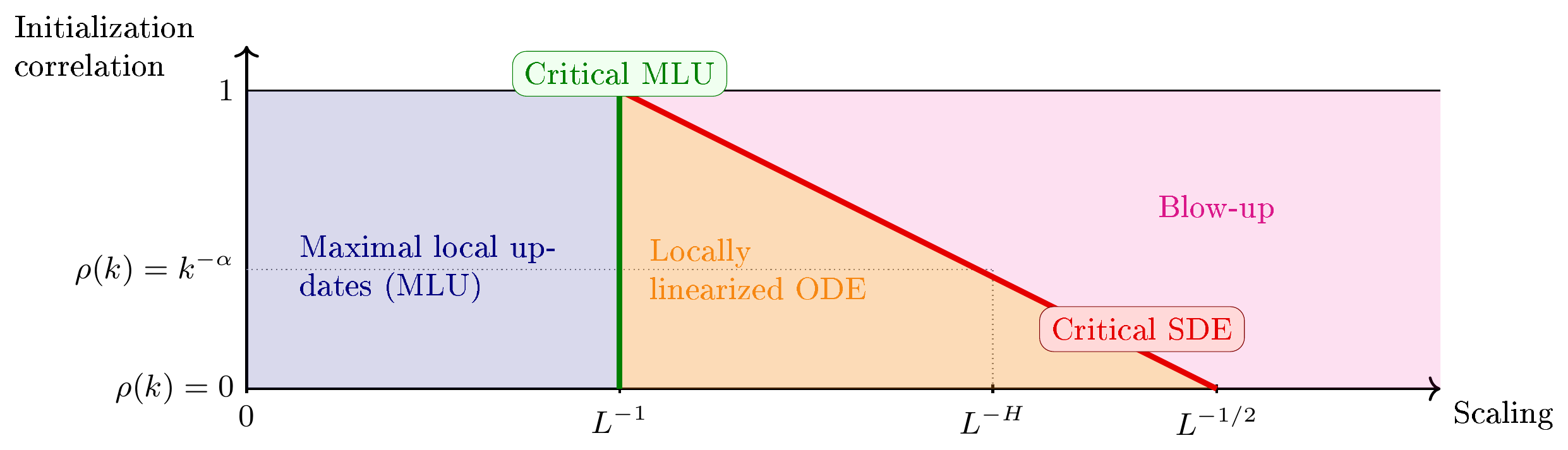
• Blow up.[^1] If $\gamma< H$, the scaling is larger than the critical scale associated with the prescribed correlation structure, and we expect the ResNet to blow up at initialization subject to suitable non-degeneracy assumptions about $\sigma$ (Rem. Remark 12). This agrees with the independent case, where the corresponding threshold is $1/2$ .
• Critical SDE (Non-trivial initialization).[^2] If #fn_ training is conjecture

[^1]: Conjecture, see Rem. Remark 12

[^2]: The behavior after training is conjecture based on Chizat's analysis for independent initialization.

$ \gamma= H=1-\frac{\alpha q}{2}, $

then and proves that the ResNet converges at initialization to the non-trivial limiting differential equation driven by the corresponding Hermite process. Based on Chizat's analysis of the training we conjecture that the parameter changes should be of order $L^{H-1}$, and hence vanish, while their accumulated first-order effect remains of order one. We therefore expect the training dynamics to be locally linearized. This would extend the "Lazy SDE" regime of [37], Fig. 4 to the correlated setting.

• Locally linearized ODE.$^{\text{Section 3.1.2}}$ If $H<\gamma<1$, the residual scaling is smaller than the critical initialization scale, and we prove that the ResNet converges to the identity at initialization (Corollary 11). At the same time, extrapolating Chizat's argument suggests parameter changes of order $L^{\gamma-1}$, which vanish as the depth diverges. To see this, combine the scaling $\lambda_L= L^{-\gamma}$ with the Taylor expansion Equation 8. We therefore conjecture a locally linearized ODE regime, analogous to the "Lazy ODE" regime of [37], Fig. 4, Thm. 2.
• Critical maximal local updates.$^{\text{Section 3.1.2}}$ At $\gamma=1$, the preceding scaling argument predicts parameter changes of order one. This corresponds to the "Maximum local update" regime of [37], Thm. 1. Here, maximal local updates means that the local features generated by an individual residual block may change by order one during training while the overall dynamics remains stable. We conjecture that an analogous regime persists under our correlated initialization. The ResNet is generally scaled to be the identity function at initialization.
• Maximal local updates (Subcritical ODE).$^{\text{Section 3.1.2}}$ For $\gamma>1$, the residual scaling is even smaller. In Chizat's setting, the corresponding subcritical MLU regime asymptotically coincides with the behavior of a network initialized with zero output weights ([37], Remark 4.2). By analogy, we conjecture a similar subcritical ODE behavior in our setting.

In summary, at initialization and and Corollary 11 rigorously characterize the critical SDE curve

$ \gamma= H=1-\frac{\alpha q}{2} $

and its subcritical side in Figure 1. The blow up-region, and the subdivision of the sub-critical region into the Locally linearized ODE, Critical MLU and MLU regimes represent a conjectural extension of Chizat's training phase diagram to correlated initialization. The resulting picture suggests, in particular, that criticality at initialization need not coincide with maximal local updates during training.

3.2 Experiments

To connect our main results to a training setting, we modify the experiments of [16], Fig. 9 and reproduce their experiment on trained ResNets with correlated initialization.[^3] We keep the same architecture of a ResNet of width $d=30$ and depth $L=1000$ with ReLU activation function and without inner weights $w_l$ trained on the MNIST dataset. While they initialized the inner weights $v_l$ directly with increments of a fractional Brownian motion, we use the Cauchy correlation function

[^3]: Our fork of their code is available at https://github.com/FelixBenning/scaling-resnets.

$ \rho(k)=(1+k)^{-\alpha}, $

which has the regularly varying behavior considered in our theoretical framework. Besides the identity feature function $\phi(x)=x$, of Hermite rank $1$, we also use the second Hermite polynomial $\phi(x)=x^2-1$, of Hermite rank $2$ . The results are shown in Figure 2.

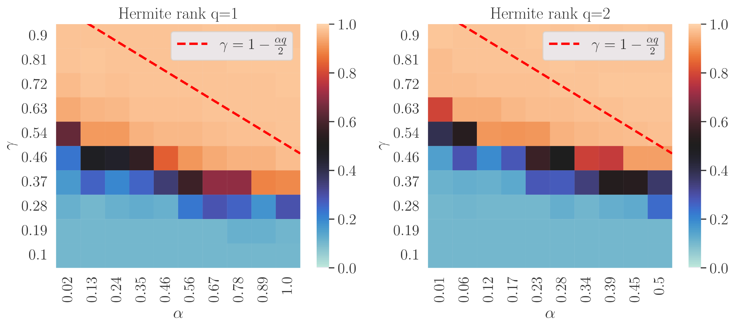
For both Hermite rank one and Hermite rank two, the low-accuracy region in blue lies predominantly below the critical curve

$ \gamma=1-\frac{\alpha q}{2} $

identified by and. This region below the curve represents the conjectured blow-up region. Larger exponents resulting in sub-critical scaling often still yield good performance. Curiously, the slope of the transition between poor and successful training neither matches the slope of the critical curve for non-trivial initialization, nor is it horizontal. A horizontal border may be expected if maximal local updates fully determined training behavior. In that case the outcome should improve as the scaling approaches $L^{-1}$ . Our experiments therefore cannot establish whether the critical initialization scaling or the maximal-local-update scaling $\lambda_L= L^{-1}$ is the more favorable choice for training.

4. Young integral equation solution theory

Section Summary: The section develops a solution theory for differential equations driven by Hölder-continuous signals that lack the smoothness needed for classical ODE methods, relying instead on Young integration to establish existence and uniqueness of solutions. It extends standard results for equations with Lipschitz coefficients to a non-homogeneous setting where the coefficient function depends on time and an auxiliary path, while also proving continuous dependence on the driving signals and initial conditions. The resulting framework is motivated by and applied to the analysis of infinite-depth residual neural networks.

The goal of this section is to develop a general solution theory for differential equations of the form

$ dx_t = \sigma(t, w_t, x_t) , dg_t \quad\text{with initial condition}\quad x_{\underline{\text{t}}} = a \in \mathcal{X}, $

where $g_t$ and $w_t$ are $\beta$ and $\alpha$ -Hölder continuous functions with exponent $\beta\in (\frac12, 1]$ and $\alpha\in (\frac12, \beta)$ . This means that classical ODE theory does not apply as the driving signal $g$ is not necessarily differentiable or of bounded variation. However it is still smooth enough for Young integration theory to be applicable. For $\beta \le \frac12$ it would become necessary to use rough path theory instead of Young integration (see e.g. [30, 32]). Differential equations of the form

$ dx_t = \sigma(x_t), dg_t $

with Lipschitz continuous $\sigma$ are already well understood both in the Young regime as well as in the rough path regime (e.g. [30] Chapter 8). Our contribution is to extend this theory to non-homogeneous $\sigma$ and prove stability results with respect to $g$, $w$ and initial conditions $a$ . An application of this theory is the infinite depth limit of residual neural networks as described in Section 2.

To distinguish between functional norms and norms on vectors, we use $|\cdot|$ as notation for the norm of vectors and reserve $| \cdot| $ for functional norms. Of course a vector in a general Banach space may be a function. Since we will however not use its properties as a function this distinction still helps make the concepts clearer. Moreover we typically write $f_s$ for function evaluation at $s$ to reserve $f(x)$ for functions that map a function $x$ to another function.

########## {caption="Definition"}

Let $(\mathcal{E}, |\cdot|)$ be a Banach space, and let $\alpha\in (0, 1]$. For a function $f\colon [\underline{\text{t}}, \overline{t}] \to \mathcal{E}$ with $\underline{\text{t}}, \overline{t} \in \mathbb{R}$ and $\underline{\text{s}}, \overline{s} \in [\underline{\text{t}}, \overline{t}]$ we define the Hölder seminorm

$ [f] {\alpha, [\underline{\text{s}}, \overline{s}]} \coloneq \sup{s\neq t \in [\underline{\text{s}}, \overline{s}]} \frac{|f_t - f_s|}{|t-s|^\alpha} \qquad\text{and}\qquad [f] _{\alpha} \coloneq [f] _{\alpha, [\underline{\text{t}}, \overline{t}]}. $

We further define the Hölder norm

$ | f| _{\alpha, [\underline{\text{s}}, \overline{s}]} \coloneq | f| _{\infty, [\underline{\text{s}}, \overline{s}]} + [f] _{\alpha, [\underline{\text{s}}, \overline{s}]} \qquad\text{and}\qquad | f| _\alpha \coloneq | f| _{\alpha, [\underline{\text{t}}, \overline{t}]} $

where $| f| {\infty, [\underline{\text{s}}, \overline{s}]} = \sup{s \in [\underline{\text{s}}, \overline{s}]} |f_s|$ is the supremum norm of $f$ on $[\underline{\text{s}}, \overline{s}]$ .

########## {caption="Definition 13: Functional spaces"}

Let $\mathcal{W}$ be a Banach space, let $T = [\underline{\text{t}}, \overline{t}]\subseteq [0, \infty)$ be a compact interval, and let $\beta\in(0, 1]$ . We denote by

$ C^\beta(T, \mathcal{W}) \coloneq \left{ w\colon T\to\mathcal{W} , :, | w| _{\beta}<\infty \right} $

the space of $\beta$ -Hölder continuous functions from $T$ to $\mathcal{W}$, equipped with the Hölder norm $| \cdot| _{\beta}$ defined above.

For the differential equation $dx_t = \sigma(t, w_t, x_t) , dg_t$ to have a unique solution, we require the following assumption, that is a generalization of Assumption 4 and Assumption 5 to the non-homogeneous case.

########## {caption="Assumption 14: Sufficiently nice function"}

Let $\mathcal{W}$, $\mathcal{V}$ and $\mathcal{X}$ be Banach spaces and let $\alpha\in (0, 1]$ . Then, the mapping

$ \sigma\colon \mathbb{R} \times \mathcal{W} \times \mathcal{X} \to \mathcal{L}(\mathcal{V}, \mathcal{X}) $

is an $\alpha$ -nice function if the following properties are verified:

• (a) $\sigma$ is bounded, that is $| \sigma| \infty < \infty$ . #it (nice function) bounded
• (b) Local Lipschitz continuity: #it_ (nice function) locally Lipschitz $\sigma(t, w, x)$ and the Fréchet derivative

$ D_x \sigma(t, w, x) \in \mathcal{L}(\mathcal{X}, \mathcal{L}(\mathcal{V}, \mathcal{X})) $

are locally Lipschitz continuous in $w$ and $x$, with local Lipschitz coefficients controlled by a continuous function $c\colon \mathbb{R}^3 \to [0, \infty)$ :

$ \begin{aligned} |\sigma(t, w, x) - \sigma(t, \tilde{w}, \tilde{x})| &\le c(t, |w|, |\tilde{w}|) \Bigl(|x-\tilde{x}|

• (1+|x|+|\tilde{x}|)|w-\tilde{w}| \Bigr) \ |D_x \sigma(t, w, x)

• D_x \sigma(t, \tilde{w}, \tilde{x})| &\le \underbrace{ c(t, |w|, |\tilde{w}|) }_{\text{locally bounded}} \underbrace{ \Bigl(|x-\tilde{x}|

• (1+|x|+|\tilde{x}|)|w-\tilde{w}| \Bigr) }_{\text{local Lipschitz control}} . \end{aligned} $

• (c) Hölder continuity in $t$ : #it_ (nice function) locally Hölder continuous $\sigma(\cdot, w, x)$ and $D_x \sigma(\cdot, w, x)$ are locally $\alpha$ -Hölder continuous in $t$, with local Hölder coefficients controlled by a continuous function $\mathsf c\colon \mathbb{R} \to [0, \infty)$ :

$ \begin{aligned} |\sigma(t, w, x) - \sigma(s, w, x)| &\le \mathsf{c}(|w|)(1+|x|)|t-s|^{\alpha} \ |D_x \sigma(t, w, x)

• D_x \sigma(s, w, x)| &\le \underbrace{ \mathsf{c}(|w|)(1+|x|) }_{\text{locally bounded}} |t-s|^{\alpha}. \end{aligned} $

Finally, an optional assumption on the Fréchet derivative of $\sigma$ with respect to $w$ instead of $x$ is given by

• (a) Differentiability in $w$ : #it_ extra assumption there exists a continuous function $\tilde{c} \colon \mathbb{R}^5 \to [0, \infty)$ and $\tilde{\mathsf c} \colon \mathbb{R}^2 \to [0, \infty)$ such that the Fréchet derivative

$ D_w \sigma(t, w, x) \in \mathcal{L}(\mathcal{W}, \mathcal{L}(\mathcal{V}, \mathcal{X})) $

is locally Lipschitz continuous in the sense

$ \begin{aligned} |D_w \sigma(t, w, x)

• D_w \sigma(t, \tilde{w}, \tilde{x})| &\le \tilde{c}(t, |w|, |\tilde{w}|, |x|, |\tilde{x}|) \Bigl(|x-\tilde{x}| + |w-\tilde{w}| \Bigr) \ |D_w \sigma(t, w, x)
• D_w \sigma(s, w, x)| &\le \tilde{\mathsf c}(|w|, |x|) |t-s|^\alpha . \end{aligned} $

########## {caption="Remark: Merging $t$ into $w$ "}

While we assume local Lipschitz continuity in $w$, we only assume local Hölder continuity in $t$ . For this reason, it is not trivial to merge $t$ into $w$ . If one were to embed $t$ into the function space $L^p([0, T], \mathbb{R})$ with $p=\frac1\alpha$ via $t\mapsto \mathbf{1}{[0, t]}$, then Lipschitz continuity translates to $\alpha$ -Hölder continuity in $t$ as $| \mathbf{1}{[0, t]}-\mathbf{1}_{[0, s]}| {L^p} = |t-s|^\alpha$, such that in place of $(t, w)$ one may consider the parameter $\tilde{w} = (\mathbf{1}{[0, t]}, w)$ . This may allow for an alternative proof where $t$ is merged into $w$, but the translation is a bit awkward and we choose the more direct approach in the following.

Theorem 15 below is one of the main theoretical contributions of the paper.

########## {caption="Remark"}

For the reader's convenience, we formally clarify the meaning of the differential equation 10 below; see e.g. [32, 30] for further details. A path $x\in C^\alpha([\underline{\text{t}}, \overline{t}], \mathcal{X})$ is a solution of Equation 10 if

$ x_t

a+\int_{\underline{\text{t}}}^t \sigma(s, w_s, x_s), dg_s, \qquad t\in[\underline{\text{t}}, \overline{t}], $

where the integral is understood in the Young sense. More precisely,

$ \int_{\underline{\text{t}}}^t \sigma(s, w_s, x_s), dg_s \coloneq \lim_{|\pi|\to0} \sum_{[u, v]\in\pi} \sigma(u, w_u, x_u)(g_v-g_u), $

where $\pi$ ranges over partitions of $[\underline{\text{t}}, t]$ and $|\pi|$ denotes the mesh of the partition. Under the assumptions of Theorem 15, the map $s\mapsto \sigma(s, w_s, x_s)$ is $\alpha$ -Hölder continuous, while $g$ is $\beta$ -Hölder continuous, and $\alpha+\beta>1$ ; hence the Young integral above is well defined. Whenever Equation 10 admits a unique solution for every initial condition, one defines the solution flow

$ \psi(, \cdot, ; s, t)\colon \mathcal{X}\to\mathcal{X}, \qquad 0\le s\le t\le T, $

by $\psi(a; s, t) \coloneq x_t^{s, a}$, where $x^{s, a}$ denotes the unique solution of Equation 10 starting from $a\in\mathcal{X}$ at time $s$, that is,

$ x_r^{s, a}

a+\int_s^r \sigma(u, w_u, x_u^{s, a}), dg_u, \qquad r\in[s, T]. $

By uniqueness the flow satisfies

$ \psi(a; s, s) = a, \qquad \psi(, \cdot, ; s, t) = \psi(, \cdot, ; u, t) \circ \psi(, \cdot, ; s, u), \qquad 0\le s\le u\le t\le T. $

########## {caption="Theorem 15: Differential equation solution"}

For $\beta\in (\frac12, 1]$, let $\alpha \in (\frac12, \beta)$ and assume $g\in C^\beta([0, T], \mathcal{V})$, $w \in C^\alpha([0, T], \mathcal{W})$ and let $\sigma\colon \mathbb{R} \times \mathcal{W} \times \mathcal{X} \to \mathcal{L}(\mathcal{V}, \mathcal{X})$ be an $\alpha$ -nice function (Assumption 14).

Then, for any $0\le \underline{\text{t}}<\overline{t}\le T$ the differential equation

$ dx_t = \sigma(t, w_t, x_t) , dg_t \quad\text{with initial condition}\quad x_{\underline{\text{t}}} = a \in \mathcal{X}\tag{10} $

• (i) has a unique solution #it_ existence and uniqueness $x$ with $x \in C^\alpha([\underline{\text{t}}, \overline{t}], \mathcal{X})$ .

For any $R>0$ there exist constants

$ C_{\text{flow}}^R, C_{\text{flow, loc}}^R, C_{\text{init}}^R, C_{\text{driver}}^R, C_{\text{param}}^R $

0

$ such that for all initial conditions a, b \in B(0, R), all driving signals g, \tilde{g} \in C^\beta([0, T], \mathcal{V}) with [g] _\beta, [\tilde{g}] _\beta \le R, all w, \tilde{w}\in C^\alpha([0, T], \mathcal{W}) with | w| _\alpha, | \tilde{w}| _\alpha \le R and all 0\le \underline{\text{t}}< \overline{t} \le T we have

• (i) Local flow bound: {#it_ flow bound} Let \psi be the flow starting at a\in \mathcal{X} in time \underline{\text{t}} (the solution path), then we have $

beginaligned | psi(a; underlinet, $\cdot$)| _alpha &<= C_flow^R \ _alpha, [underlinet, overlinet] &<= C_flow, loc^R |overlinet - underlinet|^beta - alpha &forall a in B(0, R), 0 <= underlinet< overlinet <= T. endalignedtag11

$

• (ii) Local Lipschitz continuity in the initial condition: Let x be the {#it_ lipschitz in initial condition} solution to the differential equation 10 with initial condition a, and y be the solution to 10 with initial condition b and the same driving signal g with [g] _\beta < R, then $

| x-y| $\alpha, [$underlinet, $\overline{t}]$ <= $C{\text{init}}^R |a-b|$ $\forall a$, b $\in B(0$, R), 0 <= underlinet< $\overline{t} \le T$.tag12

$

• (iii) Local Lipschitz continuity in the driving signal: Let x be the solution {#it_ lipschitz in driving signal} to the differential equation 10 with driving signal g, and y be the solution to 10 with driving signal \tilde{g} \in C^\beta([0, T], \mathcal{V}) and the same initial condition a\in B(0, R), then $

| x-y| $\alpha, [$underlinet, $\overline{t}]$ <= $C{\text{driver}}^{R} [g-\tilde{g}] _\beta$ $\forall g, \tilde{g} \in C^\beta([0$, T], $\mathcal{V}): [g] _\beta, [\tilde{g}] _\beta \le R$.

$ And with the optional Assumption 14 the theorem

• (i) Local Lipschitz continuity in the parameters: {#it_ lipschitz in parameters} Let x be the solution to the differential equation 10 with parameters w, and y be the solution to 10 with parameters \tilde{w} and the same initial condition a\in B(0, R) and the same driving signal g with [g] _\beta < R, then $

| x-y| $\alpha, [$underlinet, $\overline{t}]$ <= $C{\text{param}}^R$ | w-$\tilde{w}$| _$\alpha$ $\forall w, \tilde{w} \in C^\alpha([0$, T], $\mathcal{W})$: | w| _$\alpha$, | $\tilde{w}$| _$\alpha \le R$.

$ A direct consequence of the previous statement is that the solution of the differential equation is locally Lipschitz continuous in all input arguments. $

########## {caption="Corollary 16: Solution is locally Lipschitz in inputs"}

Assume that Assumption 14, including the optional condition, holds.

For $\beta\in (\frac12, 1]$ and $\alpha \in (\frac12, \beta)$ let

$ \Psi_\alpha \colon \begin{cases} C^\beta([0, T], \mathcal{V}) \times C^\alpha([0, T], \mathcal{W}) \times \mathcal{X} &\to C^\alpha([0, T], \mathcal{X}) \ (g, w, a) &\mapsto \Psi_\alpha(g, w, a) \end{cases} $

be the map that maps the driving signal $g$, the parameters $w$ and the initial condition $a$ to the unique solution $\Psi_\alpha(g, w, a)$ of the differential equation 10.

Then $\Psi_\alpha$ is locally Lipschitz continuous, where the space $C^\beta([0, T], \mathcal{V}) \times C^\alpha([0, T], \mathcal{W}) \times \mathcal{X}$ is equipped with the norm

$ | (g, w, a)| = | g| _\beta + | w| _\alpha + |a|. $

Without the optional assumption local Lipschitz continuity in $g$ and $a$ remains.

Proof of Corollary 16: Let $\theta = (g, w, a)$ and define $R \coloneq \max{ 2| \theta|, 1} $ . Then for all $\tilde{\theta} = (\tilde{g}, \tilde{w}, \tilde{a})$ with $| \tilde\theta - \theta| < \frac{R}2$ we have

$ [\tilde{g}] _\beta \le | \tilde{g}| _\beta \le | \tilde{g} - g| _\beta + | g| _\beta \le \tfrac{R}2 + | g| _\beta \le R $

and similarly, $| \tilde{w}| _\alpha \le R$ and $|\tilde{a}| \le R$ . Thus, we can apply Theorem 15 to obtain

$ \begin{aligned} | \Psi_\alpha(\tilde{\theta}) - \Psi_\alpha(\theta)| \alpha &\overset{\Delta}{\le} | \Psi\alpha(\tilde{g}, \tilde{w}, \tilde{a}) - \Psi_\alpha(\tilde{g}, \tilde{w}, a)| _\alpha

• \ldots
• | \Psi_\alpha(\tilde{g}, w, a) - \Psi_\alpha(g, w, a)| \alpha \ &\overset{\text{Theorem 15}}{\le} C{\text{init}}^R |a-\tilde{a}| + C_{\text{driver}}^R [g-\tilde{g}] \beta + C{\text{param}}^R | w-\tilde{w}| \alpha \ &\le \underbrace{(C{\text{init}}^R + C_{\text{driver}}^R + C_{\text{param}}^R)}_{\text{loc. Lipschitz constant}} | \tilde\theta - \theta| \end{aligned} $

The arguments for local Lipschitz continuity in $g$ and $a$ without the optional condition in Assumption 14 are analogous.

Having established existence, uniqueness, and stability of the solution, we now turn to its approximation by finite discretizations. The following result shows that the piecewise-linear interpolation of the Euler scheme converges to the solution in Hölder topology, and in particular in the supremum norm. This approximation result is a key ingredient in the proof of the large-depth convergence of ResNets in Section 2.

########## {caption="Theorem 17: Euler method convergence"}

For $\beta \in (\frac12, 1]$ let $\alpha \in (\frac12, \beta)$, $g\in C^\beta([0, T], \mathcal{V})$, $w\in C^\alpha([0, T], \mathcal{W})$ and assume $\sigma(t, w, x)$ is an $\alpha$ -nice function (see Assumption 14). Let $x$ be the unique solution of the differential equation

$ dx_t = \sigma(t, w_t, x_t) , dg_t \qquad \text{with initial condition}\quad x_0 = a. $

Let $\pi = { t_0, \dots, t_n} $ be a discretization of $[0, T]$ with $0=t_0 < \dots < t_n = T$, yielding the Euler discretization of $x$ given by

$ x^\pi_{k+1} = x^\pi_k + \sigma(t_k, w_{t_k}, x^\pi_k) (g_{t_{k+1}} - g_{t_k}) \qquad \text{with initial condition}\quad x^\pi_0 = a. $

Define $|\pi|\coloneq \max_{k} |t_{k+1} - t_k|$ .

Then for any $\alpha' \in (0, \alpha)$ we have

$ \lim_{|\pi| \to 0} | \bar{x}^\pi - x| {\alpha'} = 0 \qquad\text{with}\qquad \bar{x}^\pi_t \coloneq x^\pi_k + \underbrace{\tfrac{t-t_k}{t{k+1}-t_k}(x^\pi_{k+1} - x^\pi_k)}{\text{linear interpolation}} \text{ for } t\in [t_k, t{k+1})\tag{13} $

and $\bar{x}^\pi_T \coloneq x^\pi_n$ .

Specifically, for any $\alpha \in (\frac12, \beta)$ as above, and any $R>0$, there exist $C_{Euler}^{R, \alpha} > 0$ and $\tau = \tau(R, \alpha) > 0$ such that for all $\alpha'\in (0, \alpha)$, all initial conditions $a$ with $|a|\le R$, all drivers $g$ with $[g] _\beta \le R$ and all parameters $w$ with $| w| _\alpha \le R$ we have for all discretizations $\pi$ with maximal gap $|\pi| \le \tau$

$ | \bar{x}^\pi - x| {\alpha'} \le C{\mathrm{Euler}}^{R, \alpha} |\pi|^{(1-\frac{\alpha'}{\alpha})(\alpha+\beta - 1)}. $

########## {caption="Remark: Sup-norm"}

Observe that the case $\alpha'=0$ may be viewed as corresponding to the supremum norm, for which the estimate becomes

$ | \bar{x}^\pi-x| {\infty} \le \liminf{\alpha'\to 0} | \bar{x}^\pi-x| {\alpha'} \le \limsup{\alpha'\to 0} | \bar{x}^\pi-x| {\alpha'} \le C{\mathrm{Euler}}^{R, \alpha} |\pi|^{\alpha+\beta-1}. $

In fact, the proof proceeds by first establishing this sup-norm estimate and then using it to deduce convergence in Hölder topology.

########## {caption="Remark: Discrete convergence"}

If one is not interested in the interpolation $\bar{x}$ of $x$, one can use the fact that, at the discretization points, the interpolation coincides with $x_k$, in such a way that

$ \sup_{k} |x_k^\pi - x_{t_k}| = \sup_{k} |\bar{x}{t_k}^\pi - x{t_k}| \le | \bar{x}^\pi - x| _\infty. $

Analogously, a discrete Hölder bound holds.

5. Proofs

Section Summary: The section establishes weak convergence of a sequence of interpolated, randomly initialized neural network paths to a limiting Gaussian process in a suitable Hölder space. The argument proceeds by first obtaining joint convergence of the driving noise and auxiliary weight processes via known functional limit theorems, then applying the continuous mapping theorem to the associated rough differential equation, and finally controlling the discretization error of the Euler scheme while using tightness to remove conditioning on bounded events. A short verification for a concrete neural-network example confirms that the required regularity and boundedness assumptions on the vector field hold.

5.1 Proof of and

Choose a target exponent $\beta \in (\tfrac12, \min{ H-\frac1p, \beta_w})$ and the auxiliary exponents $\gamma_1, \gamma_2$ such that

$ \tfrac12 < \beta < \gamma_2 < \min{ \gamma_1, \beta_w}, \qquad \text{with} \qquad \gamma_1 < H - \tfrac1p.\tag{14} $

Note that we may choose $\beta > \frac12$ without loss of generality, even though we only assume $\beta>0$ in the theorem statement, due to the embedding of Hölder spaces and $\min{ H-\frac1p, \beta_w} > \frac12$ by assumption.

1. $\overline{z}^L \overset{d}\to \mathscr{z}^{q, H}$ in $\gamma_1$ -Hölder space: This follows directly from the functional limit theorems for correlated random walks ([33]). More specifically, Theorem 2.4 from [33] implies component-wise convergence of $\overline{z}^L$ in Hölder space #step_ driver convergence

$ (\overline{z}^L)^i \overset{d}\to (\mathscr{z}^{q, H})^i. $

Since these processes are independent in $i$ we obtain convergence of the entire processes $\overline{z}^L$ in the product Hölder space ([39], Thm. 2.8). Note that by independence of $\overline{z}^L$ and $\overline{w}^L$ we also have joint convergence $(\overline{z}^L, \overline{w}^L) \overset{d}\to (\mathscr{z}^{q, H}, \mathscr{w})$ in $C^{\gamma_1} \times C^{\gamma_2}$ using $\gamma_2 < \beta_w$ . 2. Convergence of Wong-Zakai approximation: For $w^L \in { \overline{w}^L, \mathscr{w}} $, depending on the initialization assumption on $w_l$, we have, by the continuous mapping Theorem (e.g. [36] Thm. 13.25),

$ \hat{h}^L \coloneq \Psi_{\beta}(\overline{z}^L, w^L, Ax) \overset{d}\to \Psi_{\beta}(\mathscr{z}^{q, H}, \mathscr{w}, Ax) = \mathscr{h}, \quad \text{in} \quad C^{\beta}([0, 1], \mathbb{R}^d),\tag{15} $

where $\Psi_{\beta}(z, w, a)$ is the continuous solution map of the differential equation

$ dh_t = \sigma(w_t, h_t) dz_t \quad \text{with} \quad h_0 = a. $

The continuity of the solution map follows directly from Corollary 16 using Assumption 4 to get continuity in $(z, a)$ and the additional regularity Assumption 5 for continuity in $(z, w, a)$ . 3. Convergence of Euler discretization: Since $h^L$ is the Euler discretization of the differential equation

$ d \hat{h}^L_s = \sigma(w^L_s, \hat{h}^L_s) d \overline{z}^L_s \quad \text{with} \quad \hat{h}^L_0 = Ax\tag{16} $

and $\overline{h}^L$ is the piecewise linear interpolation of the Euler discretization, the convergence proof of the Euler method (Theorem 17) will allow us to finish the proof. Observe that for this result to be applicable we need $w^L$ and $\overline{z}^L$ to be bounded by some $R > \max{ |Ax|, 0} $ . As a consequence, we condition on this event to get for all bounded, Lipschitz continuous functions $f\colon (C^\beta([0, 1], \mathbb{R}^d), | \cdot| _{\beta}) \to \mathbb{R}$

$ \begin{aligned} \mathsf{E}\Bigl[\bigl|f(\overline{h}^L) - f(\hat{h}^L)\bigr| \mathbf{1}_{| \overline{z}^L| _{\gamma_1} \le R, | w^L| _{\gamma_2} \le R} \Bigr] &\le \mathrm{Lip}(f)\mathsf{E}[| \overline{h}^L - \hat{h}^L| \beta \mathbf{1}{| \overline{z}^L| _{\gamma_1} \le R, | w^L| {\gamma_2} \le R}] \ &\overset{\text{Theorem 17}}{\le} \mathrm{Lip}(f)C{\text{Euler}}^{R, \gamma_2} |\tfrac1 L|^{\bigl(1-\frac{\beta}{\gamma_2}\bigr)(\gamma_2 + \gamma_1 -1)} \to 0 \quad (L \to \infty), \end{aligned}\tag{17} $

since $\frac1 L$ is the size of the discretization intervals, and the exponent is positive by the choice of auxiliary exponents in Equation 14. 4. Conclusion. For all bounded, Lipschitz continuous functions $f \colon (C^\beta([0, 1], \mathbb{R}^d), | \cdot| _{\beta}) \to \mathbb{R}$ we have for all $R > \max{ |Ax|, 0} $

$ \begin{aligned} \bigl| \mathsf{E}[f(\mathscr{h})] - \mathsf{E}[f(\overline{h}^L)]\bigr| &\le \begin{aligned}[t] \underbrace{\bigl| \mathsf{E}[f(\mathscr{h})] - \mathsf{E}[f(\hat{h}^L)]\bigr|}{\to 0 \quad \text{contin.\ solution }\mathrlap{\text{map Equation 15}}} &+ \underbrace{\mathsf{E}\bigl[\bigl|f(\hat{h}^L) - f(\overline{h}^L)\bigr| \mathbf{1}{| \overline{z}^L| _{\gamma_1} \le R, | w^L| {\gamma_2} \le R} \bigr]}{\to 0 \quad \text{Euler method conv. Equation 17}}\&+ 2| f| _\infty \mathsf{P}\bigl{ { | \overline{z}^L| _{\gamma_1} > R} \cup { | w^L| _{\gamma_2} > R} \bigr} .\end{aligned} \end{aligned} $

Consequently, we have

$ \begin{aligned} \limsup_{L \to \infty} \bigl| \mathsf{E}[f(\mathscr{h})] - \mathsf{E}[f(\overline{h}^L)]\bigr| &\le \limsup_{L \to \infty}2| f| _\infty \bigl(\mathsf{P}\bigl{ | \overline{z}^L| _{\gamma_1} > R\bigr} + \mathsf{P}\bigl{ | w^L| _{\gamma_2} > R\bigr} \bigr) \ &\to 0 \qquad (R \to \infty). \end{aligned}\tag{18} $

The convergence follows from tightness. Indeed, since $\overline{z}^L \overset{d}\to \mathscr{z}^{q, H}$ in $\gamma_1$ -Hölder space (Section 5.1), we have that (by the continuous mapping Theorem) $| \overline{z}^L| _{\gamma_1} \overset{d}\to | \mathscr{z}^{q, H}| _{\gamma_1}$ . This sequence is consequently tight in $\mathbb{R}$ by Prokhorov's theorem (e.g. [36] Thm. 13.29), which implies that

$ \lim_{R \to \infty} \sup_{L \in \mathbb{N}} \mathsf{P}{ | \overline{z}^L| _{\gamma_1} > R} = 0. $

The proof for $| w^L| _{\gamma_2}$ is analogous and follows from the definition of $w^L$ due to $\gamma_2 < \beta_w$ .

5.2 Proof of Example 6

The boundedness of $\sigma$ follows from the boundedness of $\psi$ . Since $\sigma(w, x) = \psi(Wx + b)^T \otimes \mathbb{I}_d$ we have

$ |\sigma(w, x) - \sigma(\tilde{w}, \tilde{x})| \precsim \bigl|\psi(Wx + b) - \psi(\tilde{W} \tilde{x} + \tilde{b})\bigr|, $

where $\precsim$ means that the left-hand side is upper bounded by a constant multiple of the right-hand side. This constant multiple depends on the choice of matrix norm, but always exists since all norms in finite dimension are equivalent. Let $W_i$ be the $i$ -th row vector of $W$, then, since any vector norm is equivalent to the $1$ -norm up to a constant, we have

$ \bigl|\psi(Wx + b) - \psi(\tilde{W} \tilde{x} + \tilde{b})\bigr| \precsim \sum_{i=1}^m\bigl|\psi(\langle W_i, x\rangle + b_i) - \psi(\langle \tilde{W}_i, \tilde{x}\rangle + \tilde{b}_i)\bigr|. $

For every $i$ we have

$ \begin{aligned} |\psi(\langle W_i, x\rangle + b_i) - \psi(\langle \tilde{W}_i, \tilde{x}\rangle + \tilde{b}_i)| &\le \begin{aligned}[t] &|\psi(\langle W_i, x\rangle + b_i) - \psi(\langle W_i, \tilde{x}\rangle + b_i)|\&+ |\psi(\langle W_i, \tilde{x}\rangle + b_i) - \psi(\langle \tilde{W}_i, \tilde{x}\rangle + b_i)|\&+ |\psi(\langle \tilde{W}_i, \tilde{x}\rangle + b_i) - \psi(\langle \tilde{W}_i, \tilde{x}\rangle + \tilde{b}_i)|.\end{aligned} \ &\overset{\text{Cauchy-Schwarz}}{\precsim} \mathrm{Lip}(\psi)(|W_i||x-\tilde{x}| + |\tilde{x}||W_i - \tilde{W}_i| + |b_i - \tilde{b}_i|) \ &\le c^0(|W_i|)\Bigl(|x-\tilde{x}| + (1+|x|+|\tilde{x}|)\underbrace{\bigl(|W_i - \tilde{W}_i| + |b_i - \tilde{b}i|\bigr)}{\precsim |w-\tilde{w}|}\Bigr) \end{aligned} $

with $c^0(|W_i|) \coloneq Lip(\psi)(1+|W_i|)$ . Collecting the absolute constants from the conversion of norms we have shown that there exists a continuous function $c^1(|w|)$ in $|w|$ such that

$ |\sigma(w, x) - \sigma(\tilde{w}, \tilde{x})| \le c^1(|w|)\bigl(|x-\tilde{x}| + (1+|x|+|\tilde{x}|)|w-\tilde{w}|\bigr). $

For the Fréchet derivative we proceed similarly:

$ \begin{aligned} |D_x \sigma(w, x) - D_x \sigma(\tilde{w}, \tilde{x})| &\precsim \bigl|\psi'(Wx + b)W - \psi'(\tilde{W} \tilde{x} + \tilde{b})\tilde{W}\bigr| \ &\precsim \sum_{i=1}^m\bigl|\psi'(\langle W_i, x\rangle + b_i)W_i - \psi'(\langle \tilde{W}_i, \tilde{x}\rangle + \tilde{b}_i)\tilde{W}_i\bigr|. \end{aligned} $

This additional $W_i$ factor does not pose a problem, as we can reduce it to the previous case with $\psi'$ instead of $\psi$ using the triangle inequality

$ \begin{aligned} &\bigl|\psi'(\langle W_i, x\rangle + b_i)W_i - \psi'(\langle \tilde{W}_i, \tilde{x}\rangle + \tilde{b}_i)\tilde{W}_i\bigr| \ &\le \underbrace{\bigl|\psi'(\langle W_i, x\rangle + b_i) - \psi'(\langle \tilde{W}_i, \tilde{x}\rangle + \tilde{b}i)\bigr|}{ \precsim \mathrm{Lip}(\psi')(|W_i||x-\tilde{x}| + |\tilde{x}||W_i - \tilde{W}_i| + |b_i - \tilde{b}_i|) }|W_i|

• \underbrace{\bigl|\psi'(\langle \tilde{W}_i, \tilde{x}\rangle + \tilde{b}i)\bigr|}{\le \mathrm{Lip}(\psi)}|W_i - \tilde{W}_i|. \end{aligned} $

This yields for some constant $c^2(|w|)$ that depends continuously on $|w|$ that

$ |D_x \sigma(w, x) - D_x \sigma(\tilde{w}, \tilde{x})| \le c^2(|w|)\bigl(|x-\tilde{x}| + (1+|x|+|\tilde{x}|)|w-\tilde{w}|\bigr). $

Putting everything together, we infer that Assumption 4 is satisfied, with the function $c(|w|) \coloneq \max{ c^1(|w|), c^2(|w|)}$ . The proof of the additional regularity Assumption 5 is analogous and left to the reader.

5.3 Proof of

Theorem 15

For existence and uniqueness of the solution we will use the Banach fixed point theorem. Specifically, we will construct time intervals $[t_k, t_{k+1}]$ on which we show that the operator $F_k$ with

$ F_k(x)t = a_k + \int{t_k}^t f(x)_s , dg_s \qquad \text{where} \qquad f(x)_s \coloneq \sigma(s, w_s, x_s) $

has a unique fixed point. Key ingredients for this are the continuity properties of the Young integral, which are summarized in Lemma 19 and the continuity properties of $f$ summarized in Lemma 20. Using these results we prove that $F_k$ maps a suitable ball to itself (the theorem) and is a contraction on this ball (the theorem). The last step to prove existence and uniqueness will then be to glue the solutions on the small intervals together and prove Hölder continuity. The key ingredient for this is.

########## {caption="Remark 18"}

Interestingly, the boundedness of $\sigma$ is used only to show that $F_k$ maps a suitable ball into itself. More precisely, it enters the proof only through the four estimates Equation 19c, Equation 20, Equation 25, and 30a. By contrast, the contraction property of $F_k$ does not rely on the boundedness of $\sigma$ .

The proofs of the stability properties are relatively short, reusing some of the machinery developed for existence and uniqueness.

5.3.1 Proof of: Existence and uniqueness

We prove that $x_t$ is the unique solution on finitely many small intervals. Define

$ \tau_k\coloneq \frac{\tau_0}{k+1}, \qquad K \coloneq \min\bigl{ n\in \mathbb{N}: \sum_{k=0}^{n-1}\tau_k\ge \overline{t}-\underline{\text{t}}\bigr}, $

where $\tau_0>0$ is to be chosen later. The number $K$ is finite since $\sum_{k=0}^\infty\tau_k=\infty$ . We set

$ t_k\coloneq \underline{\text{t}}+\sum_{l=0}^{k-1}\tau_l \quad\text{for }0\le k<K, \qquad t_K\coloneq \overline{t}. $

Thus $t_0=\underline{\text{t}}$, $t_K=\overline{t}$, and $t_{k+1}-t_k\le\tau_k$ for every $0\le k<K$ ; only the final interval may be shorter than $\tau_{K-1}$ . We set $a_0=a$ and, once the fixed point on $[t_k, t_{k+1}]$ has been constructed, use its end point as the next initial condition, $a_{k+1}\coloneq x_{t_{k+1}}$ . Using the Banach fixed point theorem we will construct $\alpha$ -Hölder continuous solutions on each interval. These are then glued together to obtain a solution on $[\underline{\text{t}}, \overline{t}]$ and we show uniqueness and Hölder continuity of the solution on the entire interval $[\underline{\text{t}}, \overline{t}]$ .

1. The Banach fixed point theorem on small intervals. #step_ banach fixed point

On each interval $[t_k, t_{k+1}]$ we want to show that the operator $F_k$ with

$ F_k(x)t = a_k + \int{t_k}^t f(x)_s , dg_s \qquad \text{where} \qquad f(x)_s = \sigma(s, w_s, x_s) $

has a unique fixed point.

Define $| \cdot| _{\infty, k} \coloneq | \cdot| {\infty, [t_k, t{k+1}]}$ and $[\cdot] _{\alpha, k} \coloneq [\cdot] {\alpha, [t_k, t{k+1}]}$, and the helper function

$ h\colon \begin{cases} \mathbb{N} \to \mathbb{R} \ n \mapsto n^{1-\alpha}\log(n)^\alpha. \end{cases} $

Then

$ n^{-\alpha}(1+h(n)) = \Bigl(n^{-\alpha}+\frac{\log(n)^\alpha}{n^{2\alpha -1}}\Bigr) \to 0 \implies K_h \coloneq \sup_{n\in \mathbb{N}}n^{-\alpha}(1+h(n)) < \infty. $

With the constant above and the constant $C_{\alpha, \beta}$ from Lemma 19 we may now choose the initial interval size $\tau_0$

$ \tau_0 = \min\Bigl{ 1, \bigl(\frac{\eta}{(| \sigma| \infty + C{\alpha, \beta} {c_{1}} K_h T^\alpha)R}\bigr)^{\frac1{\beta-\alpha}}, (2 K_h {c_{2}})^{-\frac1\beta} \Bigr}, $

where $\eta$ and $c_{1}$ are defined in below and $c_{2}$ is defined in below.

This choice of $\tau_0$ ensures that the and are in force.

########## {caption="Remark: Constants"}

The constants are chosen so that they do not depend on the initial point $a$, the driving signal $g$ or the parameters $w$ as long as they are bounded by $R$ .

Finally, $\eta$ is only a variable for the uniqueness argument in Section 5.3.1.

After it is established that the solution is unique we can choose $\eta=1$ without loss of generality to obtain constants independent of $\eta$ .

########## {caption="Lemma: $F_k$ maps the ball to itself"}

For all $\eta > 0$ selected independently of $k$

$ x\in B_k \coloneq B_k(\eta) \coloneq \bigl{ x\colon [t_k, t_{k+1}]\to \mathcal{X} \mid x_{t_k} = a_k, [x] _{\alpha, k} \le \eta\bigr} $

we have for all starting points with $|a| \le R$ and all $g$ with $[g] _\beta \le R$

$ \begin{aligned} \quad\text{(a)} |a_{k+1}| \le | x| {\infty, k} &\le {c{0}}(1+h(k+1)) & {c_{0}} &\coloneq R + \eta\bigl(1+\tfrac1{\log(2)}\bigr)^\alpha \ \quad\text{(b)} [f(x)] {\alpha, k} &\le {c{1}}(1+h(k+1)) & {c_{1}} & \coloneq {c_{12}}(1+\eta +{c_{0}}) \ \quad\text{(c)} {| f(x)| _{\infty, k}} &{\le | \sigma| _\infty}. \end{aligned}\tag{19} $

As a consequence, for any $\tau_0 \le \min{ 1, \bigl(\frac{\eta}{(| \sigma| \infty + C{\alpha, \beta} {c_{1}} K_h T^\alpha)R}\bigr)^{\frac1{\beta-\alpha}}} $ we have

$ [F_k(x)] _{\alpha, k} \le \eta \qquad\text{and thereby}\qquad F_k(B_k) \subseteq B_k. $

Proof: For the first claim 19a a, observe that by $\tau_0 \le 1$

$ \sum_{l=0}^{k-1} \tau_l^\alpha \le k\Bigl(\frac1k\sum_{l=0}^{k-1} \tau_l^\alpha\Bigr) \overset{\text{Jensen}}\le k\Bigl(\frac1k\sum_{l=0}^{k-1} \tau_l\Bigr)^\alpha \le k^{1-\alpha} \Bigl(\sum_{l=0}^{k-1} \frac{\tau_0}{l+1}\Bigr)^\alpha \overset{\tau_0 \le 1}\le k^{1-\alpha} \Bigl(1+\log(k)\Bigr)^\alpha. $

Consequently, for all $k\ge 1$ and $x \in B_{k-1}$ we have,

$ \begin{aligned} | x| {\infty, k-1} = \sup{t\in[t_{k-1}, t_{k}]} |x_t| &\le |a_{k-1}| + [x] {\alpha, k-1} (t{k} - t_{k-1})^\alpha \le |a_{k-1}| + \eta\tau_{k-1}^\alpha \ &\overset{\text{induction}}{\le} |a_0| + \eta\sum_{l=0}^{k-1} \tau_l^\alpha \le R + \eta k^{1-\alpha} \Bigl(1+\log(k)\Bigr)^\alpha \le {c_{0}} (1+ h(k)). \end{aligned} $

The last inequality follows from $R + \eta\le {c_{0}}$ for $k=1$ and for $k\ge 2$ we use

$ k^{1-\alpha} \Bigl(1+\log(k)\Bigr)^\alpha \le \bigl(1+\tfrac1{\log(2)}\bigr)^\alpha \underbrace{k^{1-\alpha}\log(k)^\alpha}_{=h(k)}. $

For the second claim 19a b we use local boundedness of $f$ from Lemma 20, specifically,

$ [f(x)] {\alpha, k} \overset{\text{Lemma 20}}\le {c{12}}(1+| x| {\alpha, k}) = {c{12}}(1+ \underbrace{[x] {\alpha, k}}{\le \eta} + \underbrace{| x| {\infty, k}}{ \le {c_{0}}(1+ h(k)) }) \le {c_{1}}(1+h(k)) $

with ${c_{1}} = {c_{12}}(1+\eta +{c_{0}})$ .

The third claim 19a c follows immediately from the boundedness of $\sigma$ : by the definition of $f$

$ |f(x)_s| = |\sigma(s, w_s, x_s)| \le | \sigma| _\infty. $

This bound finally implies that for any $x\in B_k$ and $s, t \in [t_k, t_{k+1}]$ using the continuity of Young integrals from Lemma 19

$ \begin{aligned} \frac{|F_k(x)_t - F_k(x)_s|}{|t-s|^\alpha} = \frac{\Bigl|\int_s^t f(x)_u , dg_u\Bigr|}{|t-s|^\alpha} &\overset{\text{Lemma 19}}{\le} (\underbrace{|f(x)s|}{\le {| \sigma| _{\infty}}}

• C_{\alpha, \beta} \underbrace{[f(x)] {\alpha, k} |t-s|^\alpha}{\le {c_{1}}(1+h(k+1)) \tau_k^\alpha}) [g] \beta \underbrace{|t-s|^{\beta-\alpha}}{\le \tau_k^{\beta-\alpha}} \ &\overset{\tau_k=\frac{\tau_0}{k+1}}{\le} (| \sigma| \infty + C{\alpha, \beta} {c_{1}} K_h \tau_0^\alpha)[g] _\beta \bigl(\tfrac{\tau_0}{k+1}\bigr)^{\beta-\alpha} \ &\le \eta. \end{aligned}\tag{20} $

For the last equation we use $[g] \beta \le R$ and the choice $\tau_0 \le \min{ 1, \bigl(\frac{\eta}{(| \sigma| \infty + C{\alpha, \beta} {c{1}} K_h T^\alpha)R}\bigr)^{\frac1{\beta-\alpha}}} $ .

This proves $[F_k(x)] _{\alpha, k} \le \eta$ and thus $F_k(x) \in B_k$, that is: $F_k$ maps $B_k$ to itself.

########## {caption="Lemma: $F_k$ is a contraction"}

Assume $[g] \beta \le R$ and let $\tau_0 \le \min{ 1, (2 K_h {c{2}})^{-\frac1\beta}}$ with

$ {c_{2}} \coloneq 2{c_{11}}(1 + \eta + {c_{0}})(1+ C_{\alpha, \beta})R. $

Let $x, y \in B_k(\eta)$ with $B_k$ as in, then $F_k$ is a contraction on $B_k$, that is

$ [F_k(y) - F_k(x)] _{\alpha, k} \le \tfrac12 [y-x] _{\alpha, k}. $

Proof: Let $x, y \in B_k$ .

Since $x_{t_k} = y_{t_k}$ we also have $f(x){t_k} = f(y){t_k}$ and therefore for all $s\in [t_k, t_{k+1}]$

$ \begin{aligned}|f(y)_s - f(x)_s| = |f(y)s - f(x)s - f(y){t_k} + f(x){t_k}| &\le [f(y) - f(x)] _{\alpha, k} |s-t_k|^\alpha\&\le [f(y) - f(x)] _{\alpha, k}\tau_k^\alpha.\end{aligned}\tag{21} $

Thus for any $s, t \in [t_k, t_{k+1}]$ we have by the continuity of Young integrals (Lemma 19)

$ \begin{aligned} &|F_k(y)_t - F_k(y)_s - F_k(x)_t + F_k(x)_s| = \Bigl|\int_s^t f(y)_u - f(x)_u , dg_u\Bigr| \ &\overset{\text{Lemma 19}}{\le} (|f(y)_s - f(x)s| + C{\alpha, \beta}[f(y) - f(x)] _{\alpha, k}|t-s|^\alpha) [g] \beta |t-s|^{\beta} \ &\overset{Equation 21}{\le} (1 + C{\alpha, \beta})[f(y) - f(x)] _{\alpha, k} [g] _\beta \tau_k^\alpha |t-s|^{\beta} \end{aligned} $

Dividing both sides by $|t-s|^\alpha$ we observe that $|t-s|^{\beta-\alpha} \le \tau_k^{\beta-\alpha}$, where we use $t_{k+1}-t_k\le \tau_k$, and therefore

$ \begin{aligned} [F_k(y)-F_k(x)] {\alpha, k} &= \sup{s\neq t \in[t_k, t_{k+1}]}\frac{|F_k(y)_t - F_k(y)_s - F_k(x)_t + F_k(x)_s|}{|t-s|^\alpha} \ &\le [f(y) - f(x)] {\alpha, k}(1 + C{\alpha, \beta}) [g] _\beta \tau_k^{\beta}. \end{aligned} $

Using $x_{t_k} = y_{t_k}$ again in Lemma 20 we get a bound on $[f(y) - f(x)] _{\alpha, k}$ of the form

$ [f(y) - f(x)] {\alpha, k} \le {c{11}} (1+ | x| _{\alpha, k} + | y| _{\alpha, k}) [y-x] _{\alpha, k}. $

Recall that by we have for $x \in B_k$

$ | x| _{\alpha, k} = [x] _{\alpha, k} + | x| {\infty, k} \le \eta + {c{0}}(1+h(k+1)) $

and therefore the same for $y\in B_k$ .

Using the constant

$ {c_{2}} = 2{c_{11}}(1 + \eta + {c_{0}})(1+ C_{\alpha, \beta})R $

and $[g] _\beta \le R$ we thus have

$ [F_k(y)-F_k(x)] _{\alpha, k} \le [y-x] {\alpha, k} {c{2}} (1+h(k+1)) \Bigl(\frac{\tau_0}{k+1}\Bigr)^{\beta} \le \tfrac12 [y-x] _{\alpha, k}. $

In the last inequality, we used $(1+h(k+1))(k+1)^{-\beta} \le K_h$ (due to $\alpha < \beta$) and the choice of $\tau_0 \le (2K_h{c_{2}})^{-\frac1\beta}$ .

Consequently $F_k$ is a contraction on $B_k$ .

2. Gluing the solutions together, uniqueness and Hölder continuity. #step_ gluing solutions together

Now we simply apply and to obtain by the Banach fixed point theorem that $F_k$ has a unique fixed point $x$ in $B_k = B_k(\eta)$ for every $k\in{ 0, \dots, K-1} $ . By concatenating the solutions on the intervals $[t_k, t_{k+1}]$ we obtain a solution on $[\underline{\text{t}}, \overline{t}]$ . So far we only know that this solution is $\alpha$ -Hölder continuous on each interval $[t_k, t_{k+1}]$ with constant $\eta$ .

########## {caption="Lemma: Hölder glue"}

Let $0\le\underline{\text{t}}<\overline{t}\le T$ and $\pi = { t_0, \dots, t_K} $ be a discretization of $[\underline{\text{t}}, \overline{t}]$, so that $t_0=\underline{\text{t}}$ and $t_K=\overline{t}$ .

Let $x\colon [\underline{\text{t}}, \overline{t}] \to \mathcal{X}$ be a function such that for all $k\in { 0, \dots, K-1} $ we have

$ [x] {\alpha, [t_k, t{k+1}]} \le \eta $

for some $\eta > 0$ . Then $x$ is $\alpha$ -Hölder continuous on $[\underline{\text{t}}, \overline{t}]$, specifically

$ [x] _{\alpha, [\underline{\text{t}}, \overline{t}]} \le \eta K^{1-\alpha}. $

Proof: To get $\alpha$ -Hölder continuity on $[\underline{\text{t}}, \overline{t}]$, let $t, s\in[\underline{\text{t}}, \overline{t}]$ (without loss of generality $t > s$). Then there exist $k, m \in { 0, \dots, K-1} $ such that $t \in [t_k, t_{k+1}]$ and $s \in [t_m, t_{m+1}]$ . The case $k=m$ is trivial so we assume $m<k$ without loss of generality. Then we have

$ \begin{aligned} |x_t - x_s| &\le |x_t - x_{t_k}| + \sum_{l=m+1}^{k-1} |x_{t_{l+1}} - x_{t_l}| + |x_{t_{m+1}} - x_s| \ &\le \eta (t-t_k)^\alpha + \sum_{l=m+1}^{k-1} \eta (t_{l+1}-t_l)^\alpha + \eta (t_{m+1}-s)^\alpha & ([x] {\alpha, [t_l, t{l+1}]} \le \eta) \ &\le \eta(k-m + 1)^{1-\alpha} (t-s)^\alpha & \Bigl(n\sum_{i=1}^n \tfrac1ny_i^\alpha \overset{\text{concave}}\le n \Bigl(\frac1n\sum_{i=1}^n y_i\Bigr)^\alpha\Bigr) \ &\le \eta K^{1-\alpha}|t-s|^\alpha \end{aligned} $

and consequently $x$ is $\alpha$ -Hölder continuous on $[\underline{\text{t}}, \overline{t}]$ with constant $\eta K^{1-\alpha}$ .

Since $\overline{t}-\underline{\text{t}}\le T$, the number $K$ of intervals in our construction is bounded by the constant

$ K\le K_T\coloneq \min\Bigl{ n\in \mathbb{N}:\sum_{k=0}^{n-1}\tau_k\ge T\Bigr} .\tag{22} $

The sequence $(\tau_k)_k$ is independent of $\underline{\text{t}}$, and so is $K_T$ . Applying therefore gives the uniform bound

$ [x] {\alpha, [\underline{\text{t}}, \overline{t}]} \le {c{3}} \coloneq \eta(K_T+1)^{1-\alpha}. $

Uniqueness of the solution follows from the Banach fixed point theorem on the ball $B_k$ . For the general case, pick two $\alpha$ -Hölder continuous solutions $x$ and $y$ of the differential equation and select $\eta = \max{ [x] _\alpha, [y] _\alpha} $ . Then by induction over $k$ we have $x, y \in B_k(\eta)$ for all $k$ and thus $x=y$ as argued above. This finishes the proof of.

5.3.2 Proof of: Local flow bound

First observe that none of the constants depend on the exact initial condition (cf. the theorem). We only used $|a| \le R$ in to define the constant ${c_{0}}$ and thereby the following constants that use it. In particular, for any initial condition $a\in B(0, R)$ we obtain uniform bounds on the solution $x$

$ \begin{alignedat}{2} | x| \alpha &= | x| \infty &&+ [x] \alpha \ &\le {c{0}}(1+h(K_T +1)) &&+ {c{3}} \eqcolon C{\text{flow}}^R \end{alignedat}\tag{23} $

where $c_{3}$ and $K_T$ are defined in Equation 22 and are independent of $\underline{\text{t}}$ by the discussion preceding. Since this constant is independent of the initial condition $a\in B(0, R)$ and the initial time $\underline{\text{t}}$ we moreover have these uniform bounds on the flow $\psi(a; \underline{\text{t}}, \cdot)$ for all $a\in B(0, R)$ and $\underline{\text{t}} \in [0, T]$, that is

$ | \psi(a; \underline{\text{t}}, \cdot)| \alpha \le C{\text{flow}}^R \qquad\forall a\in B(0, R), \underline{\text{t}} \in [0, T].\tag{24} $

This proves the bound Equation 11. For the local bound observe that we have by continuity of the Young integral (Lemma 19) and local boundedness of $f$ (Lemma 20)

$ \begin{aligned} |x_t - x_s| &= \Bigl|\int_s^t f(x)_u , dg_u\Bigr| \ &\overset{\text{Lemma 19}}{\le} (\underbrace{|f(x)s|}{\le | \sigma| _\infty}

• C_{\alpha, \beta} \underbrace{ [f(x)] \alpha }{\le {c_{12}}\mathrlap{(1+ | x| {\alpha}) \quad (\text{Lemma 20})}} |t-s|^\alpha) [g] \beta |t-s|^\beta \ &\le \underbrace{(| \sigma| \infty + C{\alpha, \beta} {c{12}}(1+ C{\text{flow}}^R) T^\alpha) R}{\eqcolon C{\text{flow, loc}}^R} |t-s|^\beta. \end{aligned}\tag{25} $

Since this is a uniform bound, we consequently have

$ [\psi(a; \underline{\text{t}}, \cdot)] {\alpha, [\underline{\text{t}}, \overline{t}]} \le C{\text{flow, loc}}^R (\overline{t}-\underline{\text{t}})^{\beta-\alpha}. $

5.3.3 Proof of: Local Lipschitz continuity in the initial condition

With $f(x)_s = \sigma(s, w_s, x_s)$ consider two solutions to the ODE $x$ and $y$ starting in $a$ and $b$ respectively, that is

$ x_t = a + \int_{\underline{\text{t}}}^t f(x)s , dg_s \qquad\text{and}\qquad y_t = b + \int{\underline{\text{t}}}^t f(y)_s , dg_s. $

We will again prove Lipschitz continuity on small intervals $[t_k, t_{k+1}]$ and then glue the bounds together to obtain Lipschitz continuity on $[\underline{\text{t}}, \overline{t}]$ . However this time it is sufficient to choose a partition $\underline{\text{t}}=t_0<\dots<t_K=\overline{t}$ whose interval lengths satisfy $t_{k+1}-t_k\le\tau$ . We may choose it such that $K\le\lceil T/\tau\rceil +1$ . Using the continuity of $f$ (Lemma 20) and the uniform bounds on $x$ and $y$ from Equation 23 we get that for all $k$

$ \begin{aligned}[f(x) - f(y)] {\alpha, k} &\le {c{12}}(1 + | x| {\alpha, k} + | y| {\alpha, k}) ([x-y] {\alpha, k} + |x{t_k}-y{t_k}|)\&\le \underbrace{{c{12}}(1+ 2C_{\text{flow}}^R)}{\eqcolon {c{4}}}([x-y] {\alpha, k}+ |x{t_k}-y_{t_k}|).\end{aligned}\tag{26} $

We will use the constant $c_{5}$ defined in Equation 29 to select $\tau \le (2{c_{5}})^{-\frac1{\beta-\alpha}}$ . Similarly to the proof of the contraction property (the theorem) we deduce, using Lemma 19,

$ \begin{aligned}|x_t - y_t - x_s + y_s| &= \Bigl|\int_s^t f(x)_u - f(y)_u , dg_u\Bigr|\&\le (|f(x)_s - f(y)s| + C{\alpha, \beta} [f(x) - f(y)] _{\alpha, k}|t-s|^\alpha) [g] _\beta |t-s|^{\beta}.\end{aligned}\tag{27} $

Since we do not have the same starting location, the bound on the difference at $s$ is less tight. However, one has the estimates

$ \begin{aligned}|f(x)s - f(y)s| &\le |f(x){t_k} - f(y){t_k}| + [f(x) - f(y)] {\alpha, k}\tau^\alpha\&= |\sigma(t_k, w{t_k}, x_{t_k}) - \sigma(t_k, w_{t_k}, y_{t_k})| + [f(x) - f(y)] {\alpha, k}\tau^\alpha\&\le \underbrace{\sup{t\in[0, T]} c(t, |w_t|, |w_t|)}{\le K_c^R}|x{t_k}-y_{t_k}| + [f(x) - f(y)] {\alpha, k}T^\alpha.\&\le \bigl(K_c^R + T^\alpha{c{4}}\bigr) \bigl([x-y] {\alpha, k} + |x{t_k}-y_{t_k}|\bigr), \end{aligned}\tag{28} $

with $K_c^R$ as defined in Lemma 20. Using Equation 28, and $[g] _\beta\le R$ , we finally get the bound

$ [x-y] {\alpha, k} \le {c{5}}([x-y] {\alpha, k} + |x{t_k}-y_{t_k}|)\tau^{\beta-\alpha} $

with

$ {c_{5}}\coloneq (K_c^R + {c_{4}}(T^\alpha + C_{\alpha, \beta} T^\alpha))R.\tag{29} $

Due to the choice of $\tau\le (2{c_{5}})^{-\frac1{\beta-\alpha}}$ we then get

$ \begin{aligned} [x-y] {\alpha, k} &\le |x{t_k}-y_{t_k}| \le (|x_{t_{k-1}}-y_{t_{k-1}}| + [x-y] {\alpha, k-1}\tau^\alpha) \ &\le (1+\tau^\alpha)|x{t_{k-1}}-y_{t_{k-1}}| \overset{\text{induction}}\le (1+ \tau^\alpha)^k |a-b| \ &\le \underbrace{(1+ \tau^\alpha)^{\lceil \frac{T}\tau\rceil }}{\eqcolon {c{6}}} |a-b|. \end{aligned} $

Recall that the number of intervals $K$ is bounded by $\lceil T/\tau\rceil +1$ and therefore we can glue the local bounds on the Hölder seminorm together using to obtain

$ [x-y] \alpha \le 2{c{6}}(\lceil \tfrac{T}\tau\rceil +1) |a-b|. $

Consequently, we have

$ \begin{aligned} | x-y| _\alpha &= | x-y| _\infty + [x-y] \alpha \ &\le |a-b| + [x-y] \alpha T^\alpha + [x-y] \alpha \le \underbrace{(1+ 2(1+T^\alpha){c{6}}(\lceil \tfrac{T}\tau\rceil +1))}{\eqcolon C{\text{init}}^R} |a-b|. \end{aligned} $

This is Lipschitz continuity in the initial condition with constant $C_{\text{init}}^R$ .

5.3.4 Proof of: Local Lipschitz continuity in the driving signal

Again, we have carefully chosen the constants to be independent of $g$ and only depending on the uniform bound $R$ . We will similarly prove Lipschitz continuity on small intervals $[t_k, t_{k+1}]$ first and then glue the bounds together to obtain Lipschitz continuity. Let $x$ and $y$ be two solutions to the ODE with

$ x_t = a + \int_{\underline{\text{t}}}^t f(x)s , dg_s \qquad\text{and}\qquad y_t = a + \int{\underline{\text{t}}}^t f(y)_s , d\tilde{g}_s. $

First observe that we already have obtained some bounds for $x, y \in B(0, R)$ and $| g| _\beta \le R$, namely

$ \begin{aligned} \quad\text{(a)} |f(x)_s| \le | f(x)| _{\infty, k} &\le {| \sigma| \infty} \ \quad\text{(b)} [f(x)] {\alpha, k} &\overset{\text{Lemma 20}}{\le} {c{12}}(1+ | x| {\alpha}) \overset{Equation 23}\le {c{12}}(1+ C{\text{flow}}^R) \end{aligned}\tag{30} $

While $x$ and $y$ are defined differently, the same arguments as in the previous section yield

$ \begin{aligned} \quad\text{(a)} |f(x)s - f(y)s| &\overset{Equation 28}{\le} \bigl(K_c^R + T^\alpha{c{4}}\bigr) \bigl([x-y] {\alpha, k} + |x{t_k}-y{t_k}|\bigr) \ \quad\text{(b)} [f(x) - f(y)] {\alpha, k} &\overset{Equation 26}{\le} {c{4}} \bigl([x-y] {\alpha, k} + |x{t_k} - y_{t_k}|\bigr). \end{aligned}\tag{31} $

Using that the Young integral is bilinear in $(f, g)$, we obtain for $s, t \in [t_k, t_{k+1}]$

$ x_t-y_t - x_s + y_s = \int_s^t f(x)_u - f(y)_u , dg_u - \int_s^t f(y)_u , d(\tilde{g}_u - g_u). $

We will now bound each term individually using Lemma 19. We have for $s, t \in [t_k, t_{k+1}]$

$ \begin{aligned} \Bigl|\int_s^t f(x)_u - f(y)_u , dg_u\Bigr| &\le \bigl(|f(x)_s - f(y)_s|

• C_{\alpha, \beta} [f(x) - f(y)] {\alpha, k}|t-s|^\alpha \bigr) [g] \beta |t-s|^{\beta} \ &\overset{Equation 31a, Equation 31b}\le \underbrace{ (K_c^R + T^\alpha{c{4}} + C{\alpha, \beta}{c_{4}} T^\alpha)R }{={c{5}} \quad Equation 29} \bigl([x-y] {\alpha, k} + |x{t_k} - y_{t_k}| \bigr) |t-s|^{\beta} \end{aligned} $

The bound on the second integral is simply

$ \begin{aligned} \Bigl|\int_s^t f(y)_u , d(\tilde{g}_u - g_u)\Bigr| &\le \bigl(|f(y)_s|

• C_{\alpha, \beta} [f(y)] {\alpha, k}|t-s|^\alpha \bigr) [\tilde{g} - g] \beta |t-s|^{\beta} \ &\overset{Equation 30a, Equation 30b}{\le} \underbrace{(| \sigma| \infty + C{\alpha, \beta} {c{12}}(1+ C{\text{flow}}^R) T^\alpha)}{\eqcolon {c{7}}} [\tilde{g} - g] _\beta |t-s|^{\beta}. \end{aligned} $

Putting everything together, we thus have

$ [x-y] {\alpha, k} \le \max{ {c{5}}, {c_{7}}} (|x_{t_k} - y_{t_k}| + [x-y] _{\alpha, k} + [\tilde{g} - g] _\beta) \tau^{\beta-\alpha} $

and, for $\tau \le (2\max{ {c_{5}}, {c_{7}}})^{-\frac1{\beta-\alpha}}$, we thus obtain

$ \begin{aligned} [x-y] {\alpha, k} &\le |x{t_k} - y_{t_k}| + [\tilde{g} - g] \beta \ &\le |x{t_{k-1}} - y_{t_{k-1}}| + [x-y] {\alpha, k-1}\tau^\alpha + [\tilde{g} - g] \beta \ &\le (1+\tau^\alpha)\Bigl(|x{t{k-1}} - y_{t_{k-1}}| + [\tilde{g} - g] \beta\Bigr) \ &\le (1+\tau^\alpha)^k \Bigl(\underbrace{|x{t_0} - y_{t_0}|}{=0} + [\tilde{g} - g] \beta\Bigr) \le \underbrace{(1+\tau^\alpha)^{\lceil \frac{T}\tau\rceil }}{\eqcolon {c{8}}} [\tilde{g} - g] _\beta. \end{aligned} $

With the same arguments as before we can glue the local bounds on the Hölder seminorm together to obtain

$ [x-y] {\alpha} \le 2(\lceil \tfrac{T}\tau\rceil +1){c{8}}[\tilde{g} - g] _\beta, $

and therefore

$ | x-y| \alpha = | x-y| \infty + [x-y] \alpha \le \underbrace{2(1+T^\alpha)(\lceil \tfrac{T}\tau\rceil +1){c{8}}}{\eqcolon C{\text{driver}}^R} [\tilde{g} - g] _\beta, $

which is Lipschitz continuity in the driving signal.

5.3.5 Proof of: local Lipschitz continuity in the parameters

With $f(w, x)_s = \sigma(s, w_s, x_s)$ consider two solutions to the ODE $x$ and $y$ with the same initial condition $a$ and driving signal $g$ but different parameters $w$ and $\tilde{w}$ respectively, that is

$ x_t = a + \int_{\underline{\text{t}}}^t f(w, x)s , dg_s \qquad\text{and}\qquad y_t = a + \int{\underline{\text{t}}}^t f(\tilde{w}, y)_s , dg_s. $

The proof is now very similar to that of and. Using $\tilde{R} \coloneq C_{\text{flow}}^R$ as a uniform bound on the solutions $x$ and $y$, we have by Lemma 20:

$ \begin{aligned} [f(w, x) - f(\tilde{w}, y)] _{\alpha, k} &\le [f(w, x) - f(w, y)] {\alpha, k} + [f(w, y) - f(\tilde{w}, y)] {\alpha, k} \ &\le {c{11}}(1+2\tilde{R})\bigl([x-y] {\alpha, k} + |x{t_k}-y{t_k}|\bigr)

• {c_{13}} | w-\tilde{w}| _{\alpha}. \end{aligned} $

And we have

$ \begin{aligned} |f(w, x)_s - f(\tilde{w}, y)s| &= |\sigma(s, w_s, x_s) - \sigma(s, \tilde{w}s, y_s)| \ &\overset{\text{Assmpt.Assumption 14}}{\le} K_c^R \bigl(|x_s - y_s| + (1+2\tilde{R})|w_s - \tilde{w}s|\bigr) \ &\le K_c^R \bigl([x-y] {\alpha, k} T^\alpha + |x{t_k} - y{t_k}| + (1+2\tilde{R})| w-\tilde{w}| {\alpha}\bigr) \ &\le \underbrace{ K_c^R\max{ 1, T^\alpha, (1+2\tilde{R})} }{\eqcolon {c{9}}}\bigl([x-y] {\alpha, k} + |x{t_k} - y{t_k}| + | w-\tilde{w}| _{\alpha} \bigr) \end{aligned} $

Thus, we have by Lemma 19:

$ \begin{aligned} |x_t - y_t - x_s + y_s| &= \Bigl|\int_s^t f(w, x)_u - f(\tilde{w}, y)_u , dg_u\Bigr| \ &\le \bigl(|f(w, x)_s - f(\tilde{w}, y)s| + C{\alpha, \beta} [f(w, x) - f(\tilde{w}, y)] {\alpha, k}|t-s|^\alpha \bigr) [g] \beta |t-s|^{\beta}. \ &\le {c{10}} \Bigl([x-y] {\alpha, k} + |x{t_k} - y{t_k}| + | w-\tilde{w}| _{\alpha}\Bigr)|t-s|^{\beta}. \end{aligned} $

with the constant

$ {c_{10}} \coloneq ({c_{9}} + C_{\alpha, \beta}\max{ {c_{11}}(1+2\tilde{R}), {c_{13}}} T^\alpha)R. $

With $t_{k+1} - t_k \le \tau$, we thus get

$ [x-y] {\alpha, k} \le {c{10}}\Bigl([x-y] {\alpha, k} + |x{t_k} - y_{t_k}| + | w-\tilde{w}| _{\alpha}\Bigr)\tau^{\beta-\alpha}. $

We now finish with the usual arguments. We pick $\tau \le (2{c_{10}})^{-\frac1{\beta-\alpha}}$ to get

$ \begin{aligned} [x-y] {\alpha, k} &\le |x{t_k} - y_{t_k}| + | w-\tilde{w}| {\alpha} \ &\le |x{t_{k-1}} - y_{t_{k-1}}| + [x-y] {\alpha, k-1}\tau^\alpha + | w-\tilde{w}| {\alpha} \ &\overset{ }{\le} (1+\tau^\alpha)\Bigl(|x{t{k-1}} - y_{t_{k-1}}| + | w-\tilde{w}| {\alpha}\Bigr) \ &\overset{\text{ind.}}{\le} (1+\tau^\alpha)^k \Bigl(\underbrace{|x{t_0} - y_{t_0}|}_{=0} + | w-\tilde{w}| _{\alpha}\Bigr) \le (1+\tau^\alpha)^{\lceil \frac{T}\tau\rceil } | w-\tilde{w}| _{\alpha}. \end{aligned}\tag{32} $

Again, we recall that the number of intervals $K$ is bounded by $\lceil T/\tau\rceil +1$ and therefore allows us to glue the local bounds on the Hölder seminorm together and to get

$ [x-y] _\alpha \le (1+\tau^\alpha)^{\lceil \frac{T}\tau\rceil }(\lceil \tfrac{T}\tau\rceil +1) | w-\tilde{w}| _{\alpha} $

and therefore

$ \begin{aligned} | x-y| _\alpha &= | x-y| _\infty + [x-y] \alpha \ &\le \underbrace{|x_0 - y_0|}{=0} + [x-y] \alpha T^\alpha + [x-y] \alpha \ &\le \underbrace{(1+T^\alpha)(1+\tau^\alpha)^{\lceil \frac{T}\tau\rceil }(\lceil \tfrac{T}\tau\rceil +1)}{\eqcolon C{\text{param}}^R} | w-\tilde{w}| _{\alpha}. \blacksquare \end{aligned} $

5.3.6 Technical Lemmas

########## {caption="Lemma 19: Continuity of Young integrals"}

Let $\mathcal{V}$ and $\mathcal{W}$ be Banach spaces and let $\mathcal{L}(\mathcal{V}, \mathcal{W})$ be the space of bounded linear operators from $\mathcal{V}$ to $\mathcal{W}$ equipped with the operator norm. Let $f \in C^\alpha([\underline{\text{t}}, \overline{t}], \mathcal{L}(\mathcal{V}, \mathcal{W}))$ and $g \in C^\beta([\underline{\text{t}}, \overline{t}], \mathcal{V})$ with $\alpha, \beta\in (0, 1]$ and $\alpha + \beta > 1$ . Then, there exists a constant $C_{\alpha, \beta}$ such that for all $s, t\in [\underline{\text{t}}, \overline{t}]$

$ \Bigl| \int_s^t f_u , dg_u

• f_s (g_t - g_s) \Bigr| \le C_{\alpha, \beta} [f] _{\alpha} [g] _{\beta} |t-s|^{\alpha + \beta} $

in particular

$ \Bigl| \int_s^t f_u , dg_u \Bigr| \le (|f_s| + C_{\alpha, \beta} [f] _{\alpha}|t-s|^\alpha) [g] _{\beta} |t-s|^{\beta} $

Proof: See e.g. ([40], Theorem 6.8) or ([30], Equation (4.3)).

For $T>0$ let $w\in C^\alpha([0, T], \mathcal{W})$ and for $\underline{\text{t}}, \overline{t} \in [0, T]$ let $x, y\in C^\alpha([\underline{\text{t}}, \overline{t}], \mathcal{X})$ . Define the map

$ f(x)_t \coloneq f(w, x)_t \coloneq \sigma(t, w_t, x_t). $

########## {caption="Lemma 20: Lipschitz continuity and boundedness of $f$ "}

Let $\sigma\colon \mathbb{R}\times \mathcal{W} \times \mathcal{X} \to \mathcal{L}(\mathcal{V}, \mathcal{X})$ satisfy Assumption 14, Then for every $R>0$ there exist ${c_{11}}, {c_{12}} > 0$ such that for all $w\in C^\alpha([0, T], \mathcal{W})$ with $| w| _\alpha \le R$ and all $x, y \in C^\alpha([\underline{\text{t}}, \overline{t}], \mathcal{X})$

$ \begin{aligned} \quad\text{(a)} [f(y) - f(x)] {\alpha, [\underline{\text{t}}, \overline{t}]} &\le {c{11}} (1+| x| _{\alpha, [\underline{\text{t}}, \overline{t}]}

• | y| _{\alpha, [\underline{\text{t}}, \overline{t}]}) \Bigl([y-x] {\alpha, [\underline{\text{t}}, \overline{t}]} +\min{t\in [\underline{\text{t}}, \overline{t}]}|x_t-y_t| \Bigr) \ \quad\text{(b)} [f(x)] {\alpha, [\underline{\text{t}}, \overline{t}]} &\le {c{12}}(1+| x| _{\alpha, [\underline{\text{t}}, \overline{t}]}). \end{aligned} $

And with the additional assumption ref ${it: extra assumption}$ it holds that for all R, $\tilde{R} > 0$ there exists ${c_{13}} > 0$ such that for all w, $\tilde{w} \in C^\alpha([0, T], \mathcal{W})$ with $| w $| _\alpha$, $| $\tilde{w}$ $| _\alpha \le R$ and all $x\in C^\alpha([\underline{\text{t}}, \overline{t}], \mathcal{X})$ with $| x $| _\alpha \le \tilde{R}$

$ \begin{aligned} \quad\text{(c)} [f(w, x) - f(\tilde{w}, x)] {\alpha, [\underline{\text{t}}, \overline{t}]} &\le {c{13}}| w-\tilde{w}| _\alpha . \end{aligned}\tag{33} $

Moreover the constants may be chosen as

$ \begin{aligned} {c_{11}} &\coloneq |D_x\sigma(0, 0, 0)| + 2 K_c^R(1+R)(1+T^\alpha) & K_c^R \coloneq \smash{\max_{\substack{t\in [0, T]\ r, s \in [0, R]}}} \max\bigl{ c(t, r, s), \mathsf c(r) \bigr} < \infty \ {c_{12}} &\coloneq K_c^R(1+2R) \ {c_{13}} &\coloneq |D_w \sigma(0, 0, 0)| + K_c^{R, \tilde{R}}(1+2\tilde{R} + 3R + T^\alpha) \end{aligned} $

with

$ K_{c}^{R, \tilde{R}} \coloneq \max_{\substack{t\in [0, T]\ r_w, s_w \in [0, R]\ r_x, s_x \in [0, \tilde{R}]}} \max\bigl{ \tilde{c}(t, r_w, s_w, r_x, s_x), \tilde{\mathsf c}(r_w, r_x)\bigr} < \infty. $

Proof: We first prove the local Lipschitz continuity of $f$ Equation 33a. Using $v_t^\lambda \coloneq \lambda y_t + (1-\lambda) x_t$ we have

$ \begin{aligned} &\bigl|f(y)_t - f(x)_t - f(y)_s + f(x)_s\bigr| \ &= \bigl|\sigma(t, w_t, y_t) - \sigma(t, w_t, x_t) - \sigma(s, w_s, y_s) + \sigma(s, w_s, x_s)\bigr| \ &= \biggl|\int_0^1 D_x \sigma(t, w_t, v_t^\lambda)d\lambda, (y_t-x_t) - \int_0^1 D_x \sigma(s, w_s, v_s^\lambda) d\lambda, (y_s-x_s)\biggr| \ &\le \begin{aligned}[t] \bigl|y_t-x_t &- (y_s - x_s)\bigr|\int_0^1 \bigl|D_x \sigma(t, w_t, v_t^\lambda)\bigr| d\lambda\&+ \bigl|y_s - x_s\bigr|\int_0^1 \Bigl|D_x \sigma(t, w_t, v_t^\lambda) - D_x \sigma(s, w_s, v_s^\lambda)\Bigr| d\lambda.\end{aligned} \end{aligned}\tag{34} $

1. Bound on first summand. The factor in front is bounded by

$ \bigl|y_t-x_t - (y_s - x_s)\bigr| \le [y - x] _\alpha |t-s|^\alpha.\tag{35} $

To bound the integral we use

$ |v_t^\lambda| \le \lambda|y_t| + (1-\lambda)|x_t| \le | y| _{\infty} + | x| _{\infty}\tag{36} $

to get the following bound on the Fréchet derivative

$ \begin{aligned} \bigl|D_x \sigma(t, w_t, v_t^\lambda)\bigr| &\le \underbrace{ \bigl|D_x \sigma(t, w_t, v_t^\lambda) -D_x \sigma(0, w_t, v_t^\lambda)\bigr| }_{\le \mathsf c(|w_t|) (1+|v_t^\lambda|) |t-0|^\alpha}

• \underbrace{ |D_x\sigma(0, w_t, v_t^\lambda) - D_x \sigma(0, 0, 0)| }_{ \le c(0, |w_t|, 0) \bigl(|v_t^\lambda - 0| + (1+|v_t^\lambda|+0)|w_t - 0|\bigr) }
• |D_x \sigma(0, 0, 0)| \ &\le \underbrace{\Bigl(K_c^R(1+ R + T^\alpha) + |D_x \sigma(0, 0, 0)|\Bigr)}{ \eqcolon {c{14}} }(1+ | x| _\infty + | y| _\infty) \end{aligned}\tag{37} $

using $| w| _\infty \le | w| _\alpha \le R$ . Combining Equation 37 we get the following bound on the first summand in Equation 34

$ \bigl|y_t-x_t - (y_s - x_s)\bigr|\int_0^1 \bigl|D_x \sigma(t, w_t, v_t^\lambda)\bigr| d\lambda \le {c_{14}}(1+ | x| _\infty + | y| _\infty)[y-x] _\alpha |t-s|^\alpha.\tag{38} $

2. Bound on second summand. By the triangle inequality

$ \bigl|y_s - x_s\bigr| \overset{\Delta}\le \min_{t\in [\underline{\text{t}}, \overline{t}]} |y_t-x_t| + |y_s - y_t - (x_s - x_t)| \overset{ }\le \min_{t\in [\underline{\text{t}}, \overline{t}]} |y_t-x_t| + [y - x] _\alpha T^\alpha\tag{39} $

is smaller for $s$ close to $t$, we need tighter bounds on the derivative difference than on the derivative itself. For this we use

$ \begin{aligned} |v_t^\lambda - v_s^\lambda| &\le \lambda|y_t - y_s| + (1-\lambda)|x_t - x_s| \ &\le ([y] _\alpha + [x] _\alpha) |t-s|^\alpha. \end{aligned} $

together with $|w_t - w_s| \le [w] _\alpha |t-s|^\alpha$ and the previous bound $|v_t^\lambda| \le | y| _\infty + | x| _\infty$ we get

$ \begin{aligned} &\bigl|D_x \sigma(t, w_t, v_t^\lambda) - D_x \sigma(s, w_s, v_s^\lambda)\bigr| \ &\overset{\Delta}{\le} \underbrace{ \bigl|D_x \sigma(t, w_t, v_t^\lambda) - D_x \sigma(s, w_t, v_t^\lambda)\bigr| }_{ \le \mathsf c(|w_t|) (1+|v_t^\lambda|) |t-s|^\alpha }

• \underbrace{\bigl|D_x \sigma(s, w_t, v_t^\lambda) - D_x \sigma(s, w_s, v_s^\lambda)\bigr| }_{ \le c(s, |w_t|, |w_s|) \bigl(|v_t^\lambda - v_s^\lambda|
• (1+|v_t^\lambda|+ |v_s^\lambda|)|w_t - w_s| \bigr) \mathrlap{\quad \text{(Assmpt.Assumption 14)} } } \ &\le K_c^R(1+| y| _\infty + | x| _\infty)|t-s|^\alpha
• K_c^R \bigl([y] _\alpha + [x] _\alpha + (1+2| x| _\infty + 2| y| \infty)[w] \alpha\bigr)|t-s|^\alpha \ &\le \underbrace{K_c^R(1+2R)}{ = {c{12}} } (1+ | y| _\alpha + | x| _\alpha) |t-s|^\alpha \end{aligned}\tag{40} $

using $[w] _\alpha \le | w| _\alpha \le R$ and $| x| _\alpha = | x| _\infty + [x] _\alpha$ . with Equation 40 we get the following bound on the second summand in Equation 34

$ \begin{aligned} &\bigl|y_s - x_s\bigr|\int_0^1 \Bigl|D_x \sigma(t, w_t, v_t^\lambda) - D_x \sigma(s, w_s, v_s^\lambda)\Bigr| d\lambda \ &\le \Bigl(\min_{t\in [\underline{\text{t}}, \overline{t}]} |y_t-x_t| + [y - x] \alpha T^\alpha\Bigr) {c{12}} (1+ | y| _\alpha + | x| _\alpha) |t-s|^\alpha. \end{aligned}\tag{41} $

Combining the bound on the first summand Equation 38 and second summand Equation 41 in Equation 34 we get Equation 33a, that is

$ \begin{aligned} [f(y)-f(x)] \alpha &= \sup{s\neq t\in [\underline{\text{t}}, \overline{t}]}\frac{|f(y)t - f(x)t - f(y)s + f(x)s|}{|t-s|^\alpha} \ &\le \underbrace{({c{14}} + {c{12}}T^\alpha)}{\le {c{11}}} (1+ | y| _\alpha + | x| \alpha) \Bigl(\min{t\in [\underline{\text{t}}, \overline{t}]}|y_t-x_t| + [y-x] _\alpha\Bigr) \end{aligned} $

with the constant

$ \begin{aligned} {c_{14}} + {c_{12}}T^\alpha &= |D_x\sigma(0, 0, 0)| + K_c^R(1+ R + T^\alpha) + K_c^R(1+2R) T^\alpha \ &\le |D_x\sigma(0, 0, 0)| + 2 K_c^R(1+R)(1+T^\alpha) \ &\overset{\text{def.}}{=} {c_{11}}. \end{aligned} $

For the local boundedness of $f$ Equation 33b we simply use Assumption 14 to get

$ \begin{aligned} [f(x)] {\alpha, [\underline{\text{t}}, \overline{t}]} &= \sup{s\neq t\in [\underline{\text{t}}, \overline{t}]}\frac{|\sigma(t, w_t, x_t) - \sigma(s, w_s, x_s)|}{|t-s|^\alpha} \ &\overset{\Delta}{\le} \sup_{s\neq t\in [\underline{\text{t}}, \overline{t}]}\frac{|\sigma(t, w_t, x_t) - \sigma(s, w_t, x_t)|}{|t-s|^\alpha}

• \frac{|\sigma(s, w_t, x_t) - \sigma(s, w_s, x_s)|}{|t-s|^\alpha} \ &\overset{\text{Assmpt.Assumption 14}}{\le} K_c^R(1+| x| _{\infty, [\underline{\text{t}}, \overline{t}]}) + K_c^R \Bigl([x] _{\alpha, [\underline{\text{t}}, \overline{t}]}
• (1+2| x| {\infty, [\underline{\text{t}}, \overline{t}]})\underbrace{[w] \alpha}{\le R}\Bigr) \ &\le \underbrace{K_c^R(1+2R)}{={c_{12}}} (1+ | x| _{\alpha, [\underline{\text{t}}, \overline{t}]}). \end{aligned} $

Finally, we prove the local Lipschitz continuity of $f$ in $w$ Equation 33c. The proof is similar to that of local Lipschitz continuity of $f$ in $x$ . We begin by defining the convex combination $w_t^\lambda \coloneq (1-\lambda)w_t + \lambda\tilde{w}_t$ with $\lambda \in [0, 1]$ such that

$ \begin{aligned} |w_t^\lambda - w_s^\lambda| &\le (1-\lambda)|w_t - w_s| + \lambda|\tilde{w}_t - \tilde{w}_s| \ &\le ([w] _\alpha + [\tilde{w}] _\alpha) |t-s|^\alpha \ &\le 2R |t-s|^\alpha \ |w_t^\lambda| &\le (1-\lambda)|w_t| + \lambda|\tilde{w}_t| \ &\le \max{ | w| _\infty, | \tilde{w}| _\infty} \ &\le R. \end{aligned} $

With the following bound on the Fréchet derivative using Assumption 14 the theorem and the definition of $K_c^{R, \tilde{R}}$

$ \begin{aligned} &|D_w \sigma(t, w_t^\lambda, x_t)| \ &\le \underbrace{ |D_w \sigma(t, w_t^\lambda, x_t) - D_w \sigma(0, w_t^\lambda, x_t)| }_{ \le K_c^{R, \tilde{R}} |t-0|^\alpha \le K_c^{R, \tilde{R}} T^\alpha }

• \underbrace{ |D_w \sigma(0, w_t^\lambda, x_t) - D_w \sigma(0, 0, 0)| }_{ \le K_c^{R, \tilde{R}} (|x_t| + |w_t^\lambda|) \le K_c^{R, \tilde{R}}(\tilde{R} + R) }
• |D_w \sigma(0, 0, 0)| \ &\le {c_{15}} \coloneq K_c^{R, \tilde{R}}(\tilde{R} + R + T^\alpha) + |D_w \sigma(0, 0, 0)|. \end{aligned} $

we get

$ \begin{aligned} &|f(w, x)_t - f(w, x)_s - f(\tilde{w}, x)_t + f(\tilde{w}, x)_s| \ &= |\sigma(t, w_t, x_t) - \sigma(t, \tilde{w}_t, x_t) - \sigma(s, w_s, x_s) + \sigma(s, \tilde{w}_s, x_s)| \ &= \biggl|\int_0^1 D_w \sigma(t, w_t^\lambda, x_t)d\lambda, (w_t - \tilde{w}_t) - \int_0^1 D_w \sigma(s, w_s^\lambda, x_s) d\lambda, (w_s - \tilde{w}_s)\biggr| \ &\le \begin{aligned}[t] &\underbrace{ |w_t - \tilde{w}t - (w_s - \tilde{w}s)| }{ \le [w-\tilde{w}] \alpha |t-s|^\alpha } \int_0^1 \underbrace{|D_w \sigma(t, w_t^\lambda, x_t)|}{\le {c{15}}} d\lambda\&\quad + \underbrace{|w_s - \tilde{w}s|}{ \le | w -\tilde{w}| \infty }\int_0^1 \underbrace{ |D_w \sigma(t, w_t^\lambda, x_t) - D_w \sigma(s, w_s^\lambda, x_s)| }{ \begin{aligned} & \scriptstyle \le K_c^{R, \tilde{R}}(|t-s|^\alpha + |x_t - x_s| + |w_t^\lambda - w_s^\lambda|) \mathrlap{\quad\text{(Assmpt.Assumption 14 the theorem + the theorem)}}\& \scriptstyle \le K_c^{R, \tilde{R}}(1+ [x] _\alpha + [w] _\alpha + [\tilde{w}] _\alpha)|t-s|^\alpha\& \scriptstyle \le K_c^{R, \tilde{R}}(1+\tilde{R} + 2R)|t-s|^\alpha\end{aligned} } d\lambda \end{aligned} \ &\le | w-\tilde{w}| \alpha \bigl({c{15}} + K_c^{R, \tilde{R}}(1+\tilde{R} + 2R)\bigr)|t-s|^\alpha. \end{aligned} $

And consequently

$ [f(w, x) - f(\tilde{w}, x)] \alpha \le | w-\tilde{w}| \alpha \underbrace{\bigl({c{15}} + K_c^{R, \tilde{R}}(1+\tilde{R} + 2R)\bigr)}{= {c_{13}}}. $

This proves the final claim.

5.4 Proof of

Theorem 17

The heart of the proof in sup-norm convergence is an incremental restart of the flow at the Euler method points and the fact that the flow is locally Lipschitz in the initial condition. But since we only have local Lipschitz continuity, we need to carefully construct a sufficiently large ball to encompass both the ODE solution and the Euler discretization. For a fixed $R>0$ that bounds the driver $g$, the parameter $w$ and initial condition $a$ we define

$ r(R) \coloneq 4 \max{ C_{\text{flow}}^R, R} \ge 4 | x| _\alpha.\tag{42} $

Then for all $s, t \in [0, T]$ with $|t-s| \le |\pi|$ we have by the local Hölder bound on the flow from Theorem 15 the theorem

$ \begin{aligned} |\psi(b; s, t)| &\le |b| + |\psi(b; s, t) - \psi(b; s, s)| \ &\le \frac{r(R)}2 + C_{\text{flow, loc}}^{r(R)} |\pi|^{\beta-\alpha} && \text{for}\quad |b| \le \tfrac{r(R)}2 \ &\le r(R) && \text{for}\quad |\pi| \le \bigl(\tfrac{r(R)}{2C_{\text{flow, loc}}^{r(R)}}\bigr)^{\frac1{\beta-\alpha}} \end{aligned}\tag{43} $

For $b$ and $|\pi|$ selected to satisfy Equation 43 we moreover have by Lemma 20 that for $|t-s| \le |\pi|$

$ \begin{aligned} [f(\psi(b; s, \cdot))] {\alpha, [s, t]} &\le {c{12}}(1+| \psi(b; s, \cdot)| {\alpha, [s, t]}) \ &\le {c{12}}(1+\underbrace{| \psi(b; s, \cdot)| {\infty, [s, t]}}{\le r(R) \quad Equation 43} + \underbrace{[\psi(b;s, \cdot)] {\alpha}}{\le C_{flow}^{r(R)}}) \ &\le{c_{16}}. \end{aligned}\tag{44} $

with ${c_{16}} \coloneq {c_{12}}(1+r(R) + C_{\text{flow}}^{r(R)})$ . To ensure that Equation 43 is in force we select

$ \tau \coloneq \min\bigl{ 1, \underbrace{ (\tfrac{r(R)}{2C_{\text{flow, loc}}^{r(R)}})^{\frac1{\beta-\alpha}}, (\tfrac{r(R)}{4C_{\text{Euler}}^{R, \alpha, 1}})^{\frac1{\alpha+\beta -1}} }{\text{sup-norm bound (Section 5.4)}}, \underbrace{ \tfrac12(2K{\mathrm{sew}}^R)^{-1/\beta} }_{\text{Hölder bound} \mathrlap{\text{ (Section 5.4)}}} \bigr},\tag{45} $

with $C_{\text{Euler}}^{R, \alpha, 1} \coloneq C_{\text{init}}^{r(R)} C_{\alpha, \beta} {c_{16}} R T$, where $C_{\text{init}}^{r(R)}$ and $2C_{\text{flow, loc}}^{r(R)}$ are the constants from Theorem 15 and $K_{\mathrm{sew}}^R$ is the constant from the discrete sewing lemma (Lemma 22). If we can keep the Euler discretization within the ball of radius $\frac{r(R)}2$, then for $|\pi|\le \tau$ we can apply Equation 43. This turns out to be possible. Indeed we will prove in the first step that a constant $C_{\text{Euler}}^{R, \alpha, 1}>0$ exists such that for all $|\pi| \le \tau$ we have the uniform bound

$ | x^\pi - x| {\infty, \pi} \le C{\text{Euler}}^{R, \alpha, 1} |\pi|^{\alpha+\beta -1} \qquad\text{and}\qquad | x^\pi| _{\infty, \pi} \le \tfrac{r(R)}2.\tag{46} $

with $| x^\pi - x| {\infty, \pi} \coloneq \sup{k} |x^\pi_k - x_{t_k}|$ and $| x^\pi| _{\infty, \pi} \coloneq \sup_k |x^\pi_k|$ .

1. Bound in discrete sup-norm. We prove Equation 46 by induction. That is, for all $k\in { 0, \dots, n} $ we show #step_ discrete sup-norm bound

$ |x^\pi_k - x_{t_k}| = |x^\pi_k - \psi(a; 0, t_k)| \le C_{\text{Euler}}^{R, \alpha, 1} |\pi|^{\alpha+\beta -1} \quad\text{and} \quad |x^\pi_k| \le \tfrac{r(R)}2. $

The second claim is needed to ensure we can apply Equation 43 and 44 in the induction step and we will also require this uniform bound on the Euler discretization in later proof steps.

The induction start $k=0$ is trivial, since $x^\pi_0 = a = \psi(a; 0, 0)$ . For the induction step we have

$ \begin{aligned} |x^\pi_k - \psi(a; 0, t_k)| &\le \sum_{l=1}^{k} \bigl|\psi(x^\pi_{l}; t_{l}, t_k) - \psi(x^\pi_{l-1}; t_{l-1}, t_k)\bigr| \ &\le \sum_{l=1}^k \bigl|\psi(x^\pi_{l}; t_{l}, t_k) - \psi(\psi(x^\pi_{l-1}; t_{l-1}, t_l); t_{l}, t_k)\bigr| \ &= |x^\pi_k - \psi(x^\pi_{k-1}; t_{k-1}, t_k)|

• \sum_{l=1}^{k-1} \underbrace{ \bigl|\psi(x^\pi_{l}; t_{l}, t_k) - \psi(\psi(x^\pi_{l-1}; t_{l-1}, t_l); t_{l}, t_k)\bigr| }{ \le C{\text{init}}^{r(R)} |x^\pi_l - \psi(x^\pi_{l-1}; t_{l-1}, t_l)| \qquad \mathrlap{\text{Induct. + Equation 43} } } \ &\le C_{\text{init}}^{r(R)} \sum_{l=1}^k |x^\pi_l - \psi(x^\pi_{l-1}; t_{l-1}, t_l)|. \end{aligned} $

Here $C_{\text{init}}^{r(R)}$ is the constant from the local Lipschitz continuity in the initial condition (see of Theorem 15), which is applicable since $x^\pi_l, \psi(x^\pi_{l-1}; t_{l-1}, t_l) \in B(0, r(R))$ due to 43 and the induction hypothesis. Now we may bound the individual terms

$ \begin{aligned} |x^\pi_l - \psi(x^\pi_{l-1}; t_{l-1}, t_l)| &\le \Bigl|\sigma(t_{l-1}, w_{t_{l-1}}, x^\pi_{l-1}) (g_{t_l} - g_{t_{l-1}}) - \int_{t_{l-1}}^{t_l} \sigma(s, w_s, \psi(x^\pi_{l-1}; t_{l-1}, s)) , dg_s\Bigr| \ &\overset{\text{Lemma 19}}{\le} C_{\alpha, \beta} \underbrace{\bigl[f(\psi(x^\pi_{l-1}; t_{l-1}, \cdot))\bigr] {\alpha, [t{l-1}, t_l]}}{\le {c{16}}} \underbrace{[g] \beta}{\le R} |t_l - t_{l-1}|^{\alpha + \beta}, \end{aligned} $

using Equation 44 in the last step. This bound on the individual terms together with

$ \begin{aligned} |t_l - t_{l-1}|^{\alpha+\beta} &= |t_l - t_{l-1}||t_l - t_{l-1}|^{\alpha+\beta-1} \ &\le |t_l - t_{l-1}||\pi|^{\alpha+\beta-1} \end{aligned} $

results in

$ |x^\pi_k - \psi(a; 0, t_k)| \le C_{\text{init}}^{r(R)} C_{\alpha, \beta} {c_{16}} R \underbrace{\sum_{l=1}^k |t_l - t_{l-1}|}{=t_k \le T}|\pi|^{\alpha+\beta -1} \le C{\text{Euler}}^{R, \alpha, 1} |\pi|^{\alpha+\beta -1}\tag{47} $

using the constant $C_{\text{Euler}}^{R, \alpha, 1} = C_{\text{init}}^{r(R)} C_{\alpha, \beta} {c_{16}} R T$ . This proves the first claim. Using $| x| _\infty \le \frac{r(R)}{4}$ by definition 42 we also have the second claim. Indeed we have

$ |x^\pi_k| \le |x^\pi_k - \psi(a; 0, t_k)| + |\psi(a; 0, t_k)| \le \tfrac{r(R)}{4} + | x| _\infty \le \tfrac{r(R)}{2}, $

due to $|\pi| \le (\frac{r(R)}{4C_{\text{Euler}}^{R, \alpha, 1}})^{\frac1{\alpha+\beta -1}}$ combined for the difference. This completes the induction and we thus have proved Equation 46. 2. Bound in sup-norm. Next we bound the piecewise linear interpolation $\bar{x}^\pi$ . For $t\in [t_k, t_{k+1})$ let $\lambda_t = \frac{t-t_k}{t_{k+1}-t_k}$ . Then we have

$ \bar{x}^\pi_t = (1-\lambda_t)x^\pi_{k} + \lambda_t x^\pi_{k+1} \qquad t\in [t_k, t_{k+1}). $

Define an interpolated version of the ODE solution $\bar{x}t \coloneq (1-\lambda_t)x{t_k} + \lambda_t x_{t_{k+1}}$ . Then we have

$ \begin{alignedat}{3} |\bar{x}^\pi_t - x_t| &\le |\bar{x}t^\pi - \bar{x}t| + |\bar{x}t - x_t|\&\le \lambda_t \underbrace{|x^\pi{k+1} - x{t{k+1}}|}{\le C{\text{Euler}}^{R, \alpha, 1} |\pi|^{\alpha+\beta-1}} + (1-\lambda_t) \underbrace{|x^\pi_k - x_{t_k}|}{\le C{\text{Euler}}^{R, \alpha, 1} \mathrlap{|\pi|^{\alpha+\beta-1}}} + \lambda_t \underbrace{|x_{t_{k+1}} - x_t|}{\le | x| \alpha |\pi|^\alpha} + (1-\lambda_t) \underbrace{|x{t_k} - x_t|}{\le | x| \alpha |\pi|^\alpha}\&\le C{\text{Euler}}^{R, \alpha, 1} |\pi|^{\alpha+\beta -1} + | x| \alpha |\pi|^\alpha\&\le \underbrace{(C{\text{Euler}}^{R, \alpha, 1} + C_{\text{flow}}^R \tau^{1-\beta})}{\eqcolon C{\mathrm{Euler}}^{R, \alpha, 2}}|\pi|^{\alpha+\beta -1} . \end{alignedat} $

using $| x| \alpha \le C{\text{flow}}^R$ and $|\pi| \le \tau$ in the last inequality. This proves the bound of the sup-norm

$ | \bar{x}^\pi - x| \infty \le C{\mathrm{Euler}}^{R, \alpha, 2} |\pi|^{\alpha+\beta -1} \qquad \forall |\pi| \le \tau.\tag{48} $

3. Bound of discrete Hölder semi-norm. For the bound in the Hölder norm we want to apply Lemma 21 with $\epsilon = \alpha - \alpha'$ . This requires a uniform bound on the Hölder semi-norms of $x$ and $\bar{x}^\pi$ . For $x$ we already have $[x] \alpha \le C{\text{flow}}^R$ by Theorem 15 the theorem. For the bound on $\bar{x}^\pi$ we have to work. #step_ discrete Hölder bound

From the discretization $\pi={ t_0, \dots, t_n} $ select a subset of anchors $\pi'= { T_0, \dots, T_m} $ with $T_0 = 0$, $T_m = T$ and

$ \tau \le T_i - T_{i-1} \le 2\tau, \quad\forall i \in { 1, \dots, m-1} \qquad \text{and}\qquad T_m - T_{m-1} \le 2\tau. $

This is possible since $|\pi| \le \tau$ implies there exists $t_k$ between $T_i+\tau$ and $T_i + 2\tau$ which may be selected as $T_{i+1}$ . This selection of anchors ensures that their number $m$ is uniformly bounded independent of $\pi$ . Indeed, we have

$ T \ge T_{m-1} = \sum_{i=1}^{m-1} (T_i - T_{i-1}) \ge (m-1) \tau \quad\implies\quad m \le \tfrac{T}{\tau}+1.\tag{49} $

Using $z_i \coloneq \sigma(t_i, w_{t_i}, x^\pi_i)$ and $A_{i, j} \coloneq z_i (g_{t_j} - g_{t_i})$ we may express the increments of $x^\pi$ as

$ x_j^\pi - x_i^\pi = \sum_{l=i}^{j-1} z_l (g_{t_{l+1}} - g_{t_l}) = \sum_{l=i}^{j-1} A_{l, l+1}. $

Our first step is to obtain a uniform Hölder bound on $x^\pi$ on the intervals spanned by the anchors. For this let $i, j$ be such that $[t_i, t_j) \subseteq [T_{k-1}, T_k) = [t_l, t_{l'})$ for some $k$, $l$ and $l'$ . Then we have by the discrete sewing Lemma (Lemma 22)

$ \begin{aligned} |x_j^\pi - x_i^\pi| &\le |x_j^\pi - x_i^\pi - A_{i, j}|

• |A_{i, j}| \ &= \Bigl| \sum_{l=i}^{j-1} A_{l, l+1}

• A_{i, j} \Bigr|

• |z_i (g_{t_j} - g_{t_i})| \ &\overset{\text{Lemma 22}}{\le} K_{\mathrm{sew}}^R (1+ | x^\pi| _{\alpha, [i:j]}) |t_j - t_i|^{\alpha+\beta}
• | \sigma| _\infty [g] \beta |t_j - t_i|^\beta \ &\le K{\mathrm{sew}}^R (1+ | x^\pi| _{\alpha, [l:l']}) |t_j - t_i|^{\alpha+\beta}
• | \sigma| _\infty R |t_j - t_i|^\beta, \end{aligned} $

where $| x^\pi| _{\alpha, [l:l']}\coloneq | x^\pi| _{\infty, [l:l']} + [x^\pi] _{\alpha, [l:l']}$ with

$ | x^\pi| {\infty, [l:l']} \coloneq \sup{l\le k \le l'} |x^\pi_k| \qquad \text{and}\qquad [x^\pi] {\alpha, [l:l']} \coloneq \sup{l\le i <j \le l'} \frac{|x_j^\pi - x_i^\pi|}{|t_j - t_i|^\alpha}. $

Due to $|t_j - t_i| \le |T_k - T_{k-1}| \le 2\tau$ we thus have

$ \begin{aligned} [x^\pi] {\alpha, [l:l']} &= \sup{i\neq j \in [l:l']} \frac{|x_j^\pi - x_i^\pi|}{|t_j - t_i|^\alpha} \ &\le K_{\mathrm{sew}}^R (1+ | x^\pi| _{\infty, [l:l']} + [x^\pi] _{\alpha, [l:l']}) |t_j - t_i|^{\beta}

• | \sigma| \infty R |t_j - t_i|^{\beta-\alpha} \ &\le K{\mathrm{sew}}^R (1+ r(R) + [x^\pi] _{\alpha, [l:l']}) (2\tau)^{\beta}
• | \sigma| _\infty R (2\tau)^{\beta-\alpha} \end{aligned} $

Due to the selection of $\tau \le \frac12(2K_{sew}^R)^{-1/\beta}$ in Equation 45 we have $K_{sew}^R (2\tau)^{\beta} \le \frac12$ and therefore

$ [x^\pi] {\alpha, [l:l']} \le \frac{K{\mathrm{sew}}^R (1+ r(R)) (2\tau)^{\beta} + | \sigma| \infty R (2\tau)^{\beta-\alpha}}{1 - K{\mathrm{sew}}^R (2\tau)^{\beta}} \le 1+ r(R) + 2| \sigma| _\infty R (2\tau)^{\beta-\alpha} \eqcolon M_0. $

Since this bound does not depend on $[T_{k-1}, T_k)$ we thereby have a uniform Hölder bound on $x^\pi$ on each of these intervals. Since the number of these intervals is uniformly bounded independent of $\pi$, we only need to glue these bounds together to get a uniform Hölder bound on $x^\pi$ on the entire interval $[0, T]$ . For this we use

$ \sum_{i=1}^n y_i^{\alpha} = n\sum_{i=1}^n \tfrac1n y_i^{\alpha} \overset{\substack{\text{concave}\\text{Jensen}}}\le n\Bigl(\sum_{i=1}^n \tfrac1n y_i\Bigr)^{\alpha} = n^{1-\alpha} \Bigl(\sum_{i=1}^n y_i\Bigr)^{\alpha}.\tag{50} $

In the following we will write $x_{T_k}^\pi\coloneq x_{l}^\pi$ for $T_k=t_l$ to avoid cumbersome notation. Then we have for $i, j$ with $t_i \in [T_{k-1}, T_k)$ and $t_j \in [T_{k'}, T_{k'+1})$ such that $k \le k'$

$ \begin{aligned} |x_j^\pi - x_i^\pi| &\le |x_j^\pi - x_{T_{k'}}^\pi| + \sum_{l=k}^{k'-1} |x_{T_{l+1}}^\pi - x_{T_l}^\pi| + |x_{T_{k}}^\pi - x_i^\pi| \ &\le M_0(t_j - T_{k'})^{\alpha} + M_0 \sum_{l=k}^{k'-1} (T_{l+1} - T_l)^{\alpha} + M_0 (T_k - t_i)^{\alpha} \ &\overset{Equation 50}{\le} M_0 \underbrace{(k'-k+2)^{1-\alpha}}{\le m^{1-\alpha}} (t_j - t_i)^{\alpha} \ &\overset{Equation 49}{\le} \underbrace{M_0 \bigl(\tfrac{T}{\tau}+1\bigr)^{1-\alpha}}{\eqcolon M_1} (t_j - t_i)^{\alpha}. \end{aligned} $

Due to $M_0 \le M_1$ the constant $M_1$ may also be used in the case of $t_i, t_j \in [T_{k-1}, T_k)$ and we obtain a discrete uniform Hölder bound on $x^\pi$

$ [x^\pi] {\alpha, \pi} \coloneq \sup{0\le i < j \le n} \frac{|x_j^\pi - x_i^\pi|}{|t_j - t_i|^{\alpha}} \le M_1. $

4. Bound of the Hölder norm. For the interpolation $\bar{x}^\pi$ we have for $t, s\in [t_k, t_{k+1})$

$ |\bar{x}^\pi_t - \bar{x}^\pi_s| = \frac{|t-s|}{t_{k+1}-t_k} |x^\pi_{k+1} - x^\pi_k| \le |t-s| M_1 |t_{k+1} - t_k|^{\alpha-1} \le M_1|t-s|^{\alpha}. $

And for $s\in [t_{j-1}, t_j)$ and $t\in [t_i, t_{i+1})$ with $j\le i$ we therefore get

$ \begin{aligned} |\bar{x}^\pi_t - \bar{x}^\pi_s| &\le |\bar{x}^\pi_t - x^\pi_i| + |x^\pi_i - x^\pi_j| + |x^\pi_j - \bar{x}^\pi_s| \ &\le M_1 (t-t_i)^{\alpha}

• M_1 (t_i - t_j)^{\alpha} + M_1 (t_j - s)^{\alpha} \ &\overset{Equation 50}{\le} 3^{1-\alpha}M_1 |t-s|^{\alpha}. \end{aligned} $

Put together we have using $M \coloneq \max{ 3^{1-\alpha}M_1, C_{flow}^R} \ge M_1$

$ [\bar{x}^\pi] {\alpha} = \sup{s\neq t\in [0, T]} \frac{|\bar{x}^\pi_t - \bar{x}^\pi_s|}{|t-s|^{\alpha}} \le M $

uniformly over $\pi$ . And for the solution of the differential equation $x$ we have $[x] \alpha \le C{\text{flow}}^R\le M$ by Theorem 15 the theorem. With the application of Lemma 21 with $\epsilon = \alpha - \alpha'$ we thus have

$ [\bar{x}^\pi - x] _{\alpha'} \le 2M^{\frac{\alpha'}{\alpha}} | \bar{x}^\pi - x| _\infty^{1-\frac{\alpha'}{\alpha}} $

This implies

$ \begin{aligned} | \bar{x}^\pi - x| _{\alpha'} &= | \bar{x}^\pi - x| _\infty + [\bar{x}^\pi - x] _{\alpha'} \ &\le | \bar{x}^\pi - x| _\infty + 2M^{\frac{\alpha'}{\alpha}} | \bar{x}^\pi - x| \infty^{1-\frac{\alpha'}{\alpha}} \ &\overset{\text{ }}{\le} \Bigl(C{\mathrm{Euler}}^{R, \alpha, 2} |\pi|^{\frac{\alpha'}{\alpha}(\alpha+\beta -1)}

• 2M^{\frac{\alpha'}{\alpha}} (C_{\mathrm{Euler}}^{R, \alpha, 2})^{1-\frac{\alpha'}{\alpha}}\Bigr) |\pi|^{(1-\frac{\alpha'}{\alpha})(\alpha+\beta - 1)} \ &\le \underbrace{ \max{ 1, C_{\mathrm{Euler}}^{R, \alpha, 2}} (1+ 2M) }{\eqcolon C{\mathrm{Euler}}^{R, \alpha}} |\pi|^{(1-\frac{\alpha'}{\alpha})(\alpha+\beta - 1)}, \end{aligned} $

where we use $\alpha' < \alpha$ with $M \ge M_0 \ge 1$ and $|\pi| \le \tau \le 1$ in the last inequality. $\blacksquare$

The key ingredient to turn the uniform convergence into convergence in Hölder space is the following Lemma.

########## {caption="Lemma 21: Uniform to Hölder bound"}

Let $\alpha\in (0, 1]$. For $x, y \in C^\alpha([0, T], \mathcal{X})$ assume there exists $M>0$ such that $[x] _\alpha, [y] _\alpha \le M$ ; then for all $\epsilon\in (0, \alpha)$ we have

$ [x - y] _{\alpha-\epsilon} \le 2M^{1-\frac{\epsilon}{\alpha}} | x - y| _\infty^{\frac{\epsilon}{\alpha}}. $

Proof: Let $e_t \coloneq x_t - y_t$ be the error of the approximation. Then

$ |e_t - e_s| \le |e_t| + |e_s| \le 2| e| _\infty $

and due to $[x] _\alpha, [y] _\alpha \le M$

$ |e_t - e_s| \le |x_t - x_s| + |y_t - y_s| \le 2M |t-s|^\alpha. $

This implies the error difference is bounded by the minimum and we may bound this by any combination of the two bounds. That is

$ |e_t - e_s| \le \min{ 2| e| _\infty, 2M |t-s|^\alpha} \le 2| e| _\infty^{\frac{\epsilon}{\alpha}} (M|t-s|^{\alpha})^{1-\frac{\epsilon}{\alpha}} = 2M^{1-\frac{\epsilon}{\alpha}}| x-y| _\infty^{\frac{\epsilon}{\alpha}} |t-s|^{\alpha-\epsilon}. $

But this implies $[x - y] _{\alpha-\epsilon} = [e] _{\alpha-\epsilon} \le 2M^{1-\frac{\epsilon}{\alpha}}| x-y| _\infty^{\frac{\epsilon}{\alpha}}$, which is the claim.

Discrete sewing.

To prove the necessary uniform bound on the Hölder semi-norm required for Lemma 21 the key ingredient is the discrete sewing Lemma 22.

For $z_i \coloneq \sigma(t_i, w_{t_i}, x^\pi_i)$ we define the integral approximation

$ A_{t_i, t_j} \coloneq A_{i, j} \coloneq z_i (g_{t_j} - g_{t_i}) \Bigl(\approx \int_{t_i}^{t_j} \sigma(s, w_s, x_s) , dg_s\Bigr). $

Since integrals satisfy the addition property $\int_{t_i}^{t_j} = \int_{t_i}^s + \int_s^{t_j}$ for any $s\in [t_i, t_j]$ we denote the addition defect by

$ \delta A_{i, k, j} \coloneq A_{i, j} - A_{i, k} - A_{k, j}. $

Using a bound on this addition defect (Lemma 23) we can prove the following discrete sewing lemma that is the key ingredient to obtain a uniform bound on the Hölder semi-norm of $x^\pi$ on the intervals spanned by the anchors (Section 5.4 in the proof of Theorem 17).

########## {caption="Lemma 22: Discrete sewing"}

Suppose that $\sigma$ satisfies Assumption 14 and $| w| _\alpha, [g] \beta \le R$ . Let $z_k = \sigma(t_k, w{t_k}, x^\pi_k)$ for $x^\pi_k$ and $t_k$ as defined in Theorem 17. Then, for $0\le i<j\le n$,

$ \Biggl|\sum_{k=i}^{j-1} z_k(g_{t_{k+1}} - g_{t_k}) - z_i (g_{t_j} - g_{t_i})\Biggr| = \Biggl|\sum_{k=i}^{j-1} A_{k, k+1} - A_{i, j}\Biggr| \le K_{\mathrm{sew}}^R (1+ | x^\pi| _{\alpha, [i:j]}) |t_j - t_i|^{\alpha+\beta} $

with $K_{sew}^R \coloneq \sum_{k=1}^\infty \bigl(\frac{2}{k}\bigr)^{\alpha+\beta}K_{\delta A}^R $ .

Proof: Observe that the sum over $A_{k, k+1}$ is essentially a better integral approximation than $A_{i, j}$ that corresponds to just the end-points. Let $t_0 < \dots < t_n$ be the discretization $\pi$ and

$ \pi_m \coloneq { t_i, \dots, t_j} = { u_0, \dots, u_m}, \qquad \pi_1 \coloneq { t_i, t_j} $

be two sub-partitions of the discretization $\pi$ with

$ [\pi_m] = { [t_k, t_{k+1}]: i \le k < j}, \qquad\text{and}\qquad [\pi_1] = { [t_i, t_j]} . $

We define the notation

$ S_{\pi} A \coloneq \sum_{[t, s]\in [\pi]} A_{t, s}, $

such that the quantity we want to bound is given by

$ S_{\pi_m}A - S_{\pi_1} A = \sum_{k=i}^{j-1} A_{k, k+1} - A_{i, j} = \sum_{k=i}^{j-1} z_k (g_{t_{k+1}} - g_{t_k}) - z_i (g_{t_j} - g_{t_i}). $

We will now construct $\pi_{m-1}, \dots, \pi_{2}$ by successively dropping one $t_l$ from the partition. Specifically, since

$ (m-1) \min_{0<k<m} (u_{k+1} - u_{k-1}) \le \sum_{0<k<m} (u_{k+1} - u_{k-1}) \le 2(u_m - u_0) = 2(t_j - t_i), $

we have for $l \coloneq \operatorname*{arg, min}{0<k<m} (u{k+1} - u_{k-1})$ that

$ u_{l+1} - u_{l-1} \le \tfrac{2(t_j - t_i)}{m-1}.\tag{51} $

We then define $\pi_{m-1} = \pi_m \setminus { u_l} $ and thus have

$ S_{\pi_m} A - S_{\pi_{m-1}} A = A_{u_{l-1}, u_l} + A_{u_l, u_{l+1}} - A_{u_{l-1}, u_{l+1}} = -\delta A_{u_{l-1}, u_l, u_{l+1}}. $

With Lemma 23 we thus obtain

$ \begin{aligned} |S_{\pi_m} A - S_{\pi_{m-1}} A| &= |\delta A_{u_{l-1}, u_l, u_{l+1}}| \ &\overset{\text{Lemma 23}}{\le} K_{\delta A}^R (1+ | x^\pi| {\alpha, [i:j]})|u{l+1} - u_{l-1}|^{\alpha+\beta} \ &\overset{Equation 51}{\le} 2^{\alpha+\beta} K_{\delta A}^R (1+ | x^\pi| _{\alpha, [i:j]})\frac{|t_j- t_i|^{\alpha+\beta}}{(m-1)^{\alpha+\beta}}. \end{aligned} $

Iterating this argument we get

$ \begin{aligned} |S_{\pi_m} A - S_{\pi_1} A| &\le \sum_{k=1}^{m-1} |S_{\pi_{k+1}} A - S_{\pi_k} A| \ &\le 2^{\alpha+\beta} K_{\delta A}^R (1+ | x^\pi| {\alpha, [i:j]})|t_j- t_i|^{\alpha+\beta} \sum{k=1}^{m-1} \frac{1}{k^{\alpha+\beta}} \ &\le K_{\mathrm{sew}}^R (1+ | x^\pi| _{\alpha, [i:j]})|t_j- t_i|^{\alpha+\beta} \end{aligned} $

with $K_{sew}^R \coloneq \sum_{k=1}^\infty \bigl(\frac{2}{k}\bigr)^{\alpha+\beta}K_{\delta A}^R $ .

What is left to prove is the bound on the addition defect.

########## {caption="Lemma 23: Addition defect bound"}

The addition defect is given by

$ \delta A_{i, k, j} = (z_i - z_k)(g_{t_j} - g_{t_k}) $

and if $\sigma$ satisfies Assumption 14 and $| w| _\alpha, [g] _\beta \le R$, then

$ |\delta A_{i, k, j}| \le K_{\delta A}^R(1+| x^\pi| _{\alpha, [i:j]})|t_j - t_i|^{\alpha+\beta} \qquad \forall 0\le i < k < j \le n. $

with $| x^\pi| _{\alpha, [i:j]} = | x^\pi| _{\infty, [i:j]} + [x^\pi] _{\alpha, [i:j]}$ where

$ [x^\pi] {\alpha, [i:j]} = \sup{i\le k<l \le j} \frac{|x^\pi_l - x^\pi_k|}{|t_l - t_k|^\alpha} \qquad \text{and} \qquad | x^\pi| {\infty, [i:j]} = \max{i\le k \le j} |x^\pi_k| $

and $K_{\delta A}^R \coloneq 2K_c^R(1+R) R$ .

Proof: The first claim follows directly from the definition

$ \begin{aligned} \delta A_{i, k, j} &= A_{i, j} - A_{i, k} - A_{k, j} \ &= z_i (g_{t_j} - \cancel{g_{t_i}}) - z_i (g_{t_k} - \cancel{g_{t_i}}) - z_k (g_{t_j} - g_{t_k}) \ &= (z_i - z_k)(g_{t_j} - g_{t_k}). \end{aligned} $

We thus obtain with $[g] _\beta \le R$ that

$ |\delta A_{i, k, j}| \le [z] _{\alpha, [i:j]} [g] _{\beta} |t_k - t_i|^\alpha |t_j - t_k|^\beta \le [z] _{\alpha, [i:j]} R |t_j - t_i|^{\alpha+\beta}. $

Now for $i\le k < l \le j$ we have

$ \begin{aligned} |z_l - z_k| &= \Bigl|\sigma(t_l, w_{t_l}, x^\pi_l) - \sigma(t_k, w_{t_k}, x^\pi_k)\Bigr| \ &\le |\sigma(t_l, w_{t_l}, x^\pi_l) - \sigma(t_k, w_{t_l}, x^\pi_l)|

• |\sigma(t_k, w_{t_l}, x^\pi_l) - \sigma(t_k, w_{t_k}, x^\pi_k)| \ &\overset{\text{Assmpt.Assumption 14}}{\le} K_c^R(1+ |x^\pi_l|)|t_l - t_k|^\alpha
• K_c^R \Bigl(|x^\pi_l - x^\pi_k|
• (1+|x^\pi_k|+|x^\pi_l|) |w_{t_l} - w_{t_k}| \Bigr) \ &\le K_c^R\Bigl(\bigl(1+ |x^\pi_l|+|x^\pi_k|\bigr)(1+ [w] _\alpha)+[x^\pi] _{\alpha, [i:j]}\Bigr)|t_l - t_k|^\alpha \ &\le 2K_c^R(1+R)\bigl(1+ \underbrace{| x^\pi| _{\infty, [i:j]}+[x^\pi] {\alpha, [i:j]}}{= | x^\pi| _{\alpha, [i:j]}}\bigr)|t_l - t_k|^\alpha \end{aligned} $

using $[w] _\alpha \le R$ . We thus have $[z] _{\alpha, [i:j]} \le 2K_c^R(1+R)(1+ | x^\pi| {\alpha, [i:j]})$ and by definition of $K{\delta A}^R$ the claim follows.

Acknowledgements

The experiments presented in this paper were carried out using the HPC facilities of the University of Luxembourg ([41]) – see https://hpc.uni.lu. Research supported by the Luxembourg National Research Fund (Grants: O24/18972745/GFRF and O22/17372844/FraMStA).

References

Section Summary: The references section compiles a bibliography of scholarly works cited throughout the paper. It includes foundational papers on neural network designs such as attention mechanisms and residual connections, along with studies on training stability and normalization techniques. Additional entries cover mathematical topics like stochastic processes, fractional Brownian motion, and rough path theory that underpin the paper's analysis.

[1] A. Vaswani, N. Shazeer, N. Parmar, J. Uszkoreit, L. Jones, A. N. Gomez, Ł. Kaiser, and I. Polosukhin. Attention is all you need. Advances in neural information processing systems, 30, 2017.

[2] R. K. Srivastava, K. Greff, and J. Schmidhuber. Training Very Deep Networks. In Advances in Neural Information Processing Systems, volume 28. Curran Associates, Inc., 2015.

[3] K. He, X. Zhang, S. Ren, and J. Sun. Deep residual learning for image recognition. In Proceedings of the IEEE Conference on Computer Vision and Pattern Recognition, pages 770–778, 2016a.

[4] K. He, X. Zhang, S. Ren, and J. Sun. Identity Mappings in Deep Residual Networks. In B. Leibe, J. Matas, N. Sebe, and M. Welling, editors, Computer Vision – ECCV 2016, volume 9908, pages 630–645. Springer International Publishing, Cham, 2016b. ISBN 978-3-319-46492-3 978-3-319-46493-0. doi:10.1007/978-3-319-46493-$0_38$.

[5] W. E. A Proposal on Machine Learning via Dynamical Systems. Communications in Mathematics and Statistics, 5(1):1–11, Mar. 2017. ISSN 2194-671X. doi:10.1007/s40304-017-0103-z.

[6] E. Haber and L. Ruthotto. Stable architectures for deep neural networks. Inverse problems, 34(1):014004, 2018.

[7] P. Marion, Y.-H. Wu, M. E. Sander, and G. Biau. Implicit regularization of deep residual networks towards neural ODEs. In The Twelfth International Conference on Learning Representations, Oct. 2023.

[8] S. Ioffe and C. Szegedy. Batch Normalization: Accelerating Deep Network Training by Reducing Internal Covariate Shift. In Proceedings of the 32nd International Conference on Machine Learning, pages 448–456. PMLR, June 2015.

[9] A. Brock, S. De, and S. L. Smith. Characterizing signal propagation to close the performance gap in unnormalized ResNets. In International Conference on Learning Representations, Oct. 2020.

[10] D. Arpit, V. Campos, and Y. Bengio. How to initialize your network? robust initialization for weightnorm & resnets. Advances in Neural Information Processing Systems, 32, 2019.

[11] S. De and S. Smith. Batch Normalization Biases Residual Blocks Towards the Identity Function in Deep Networks. In H. Larochelle, M. Ranzato, R. Hadsell, M. Balcan, and H. Lin, editors, Advances in Neural Information Processing Systems, volume 33, pages 19964–19975. Curran Associates, Inc., 2020.

[12] J. Shao, K. Hu, C. Wang, X. Xue, and B. Raj. Is normalization indispensable for training deep neural network? In Advances in Neural Information Processing Systems, volume 33, pages 13434–13444. Curran Associates, Inc., 2020.

[13] H. Zhang, D. Yu, M. Yi, W. Chen, and T.-Y. Liu. Stabilize deep ResNet with a sharp scaling factor $\tau$. Machine Learning, 111(9):3359–3392, Sept. 2022. ISSN 0885-6125, 1573-0565. doi:10.1007/s10994-022-06192-x.

[14] A.-S. Cohen, R. Cont, A. Rossier, and R. Xu. Scaling Properties of Deep Residual Networks. In Proceedings of the 38th International Conference on Machine Learning, pages 2039–2048. PMLR, July 2021.

[15] R. Cont, A. Rossier, and R. Xu. Asymptotic Analysis of Deep Residual Networks, Jan. 2023.

[16] P. Marion, A. Fermanian, G. Biau, and J.-P. Vert. Scaling ResNets in the Large-depth Regime. Journal of Machine Learning Research, 26(56):1–48, 2025. ISSN 1533-7928.

[17] C. A. Tudor. Analysis of variations for self-similar processes. A stochastic calculus approach. Probab. Appl. Cham: Springer, 2013. ISBN 978-3-319-00935-3; 978-3-319-00936-0. doi:10.1007/978-3-319-00936-0.

[18] C. Tudor. Non-Gaussian selfsimilar stochastic processes. SpringerBriefs Prob. Math. Stat. Cham: Springer, 2023. ISBN 978-3-031-33771-0; 978-3-031-33772-7. doi:10.1007/978-3-031-33772-7.

[19] V. Pipiras and M. S. Taqqu. Long-Range Dependence and Self-Similarity. Cambridge University Press, Apr. 2017. ISBN 978-1-107-03946-9.

[20] S. Bai and M. S. Taqqu. Sensitivity of the Hermite rank. Stochastic Processes and their Applications, 129(3):822–840, Mar. 2019. ISSN 0304-4149. doi:10.1016/j.spa.2018.03.020.

[21] K. Hayashi and K. Nakagawa. Fractional SDE-Net: Generation of Time Series Data with Long-term Memory. In 2022 IEEE 9th International Conference on Data Science and Advanced Analytics (DSAA), pages 1–10, Oct. 2022. doi:10.1109/DSAA54385.2022.10032351.

[22] L. C. Young. An inequality of the Hölder type, connected with Stieltjes integration. Acta Mathematica, 67(none):251–282, Jan. 1936. ISSN 0001-5962, 1871-2509. doi:10.1007/BF02401743.

[23] T. Lyons. Differential equations driven by rough signals (I): An extension of an inequality of L. C. Young. Mathematical Research Letters, 1(4):451–464, Aug. 1994. ISSN 1073-2780, 1945-001X. doi:10.4310/MRL.1994.v1.n4.a5.

[24] Y. Hu and D. Nualart. Differential Equations Driven by Hölder Continuous Functions of Order Greater than 1/2. In F. E. Benth, G. Di Nunno, T. Lindstrøm, B. Øksendal, and T. Zhang, editors, Stochastic Analysis and Applications, pages 399–413. Springer Berlin Heidelberg, Berlin, Heidelberg, 2007. ISBN 978-3-540-70846-9 978-3-540-70847-6. doi:10.1007/978-3-540-70847-$6_17$.

[25] A. Lejay. Controlled differential equations as Young integrals: A simple approach. Journal of Differential Equations, 249(8):1777–1798, Oct. 2010. ISSN 0022-0396. doi:10.1016/j.jde.2010.05.006.

[26] D. Nualart and A. Răşcanu. Differential equations driven by fractional Brownian motion. Collectanea Mathematica, pages 55–81, 2002.

[27] N. D. Cong, L. H. Duc, and P. T. Hong. Nonautonomous Young Differential Equations Revisited. Journal of Dynamics and Differential Equations, 30(4):1921–1943, Dec. 2018. ISSN 1040-7294, 1572-9222. doi:10.1007/s10884-017-9634-y.

[28] T. J. Lyons. Differential equations driven by rough signals. Revista Matemática Iberoamericana, 14(2):215–310, 1998.

[29] I. Bailleul. Regularity of the Itô-Lyons map. Confluentes Mathematici, 7(1):3–11, 2015. ISSN 1793-7434. doi:10.5802/cml.15.

[30] P. K. Friz and M. Hairer. A Course on Rough Paths: With an Introduction to Regularity Structures. Universitext. Springer International Publishing, Cham, 2020. ISBN 978-3-030-41555-6 978-3-030-41556-3. doi:10.1007/978-3-030-41556-3.

[31] A. M. Davie. Differential Equations Driven by Rough Paths: An Approach via Discrete Approximation. Applied Mathematics Research eXpress, 2008:40, Jan. 2008. ISSN 1687-1200. doi:10.1093/amrx/abm009.

[32] P. Friz and N. Victoir. Euler estimates for rough differential equations. Journal of Differential Equations, 244(2):388–412, Jan. 2008. ISSN 0022-0396. doi:10.1016/j.jde.2007.10.008.

[33] F. Benning and I. Nourdin. Functional Scaling Limits of Interpolated Correlated Random Walks in Hölder Topology, June 2026.

[34] F. R. Kschischang. Kronecker Product and Vectorization. 2022.

[35] I. Nourdin and G. Peccati. Normal Approximations with Malliavin Calculus: From Stein's Method to Universality. Cambridge Tracts in Mathematics. Cambridge University Press, 2012. doi:10.1017/CBO9781139084659.

[36] A. Klenke. Probability Theory: A Comprehensive Course. Universitext. Springer, London, 2014. ISBN 978-1-4471-5360-3 978-1-4471-5361-0. doi:10.1007/978-1-4471-5361-0.

[37] L. Chizat. The Hidden Width of Deep ResNets: Tight Error Bounds and Phase Diagram, Mar. 2026.

[38] N. Dey, B. Zhang, L. Noci, M. Li, B. Bordelon, S. Bergsma, C. Pehlevan, B. Hanin, and J. Hestness. Don't be lazy: CompleteP enables compute-efficient deep transformers. In Advances in Neural Information Processing Systems, volume 38, pages 137707–137739. Curran Associates, Inc., 2025.

[39] P. Billingsley. Convergence of Probability Measures. Wiley Series in Probability and Statistics. John Wiley & Sons, 2 edition, July 1999. ISBN 978-1-118-62596-5. doi:10.1002/9780470316962.

[40] P. K. Friz and N. B. Victoir. Multidimensional Stochastic Processes as Rough Paths: Theory and Applications. Cambridge Studies in Advanced Mathematics. Cambridge University Press, Cambridge, 2010. ISBN 978-0-521-87607-0. doi:10.1017/CBO9780511845079.

[41] S. Varrette, H. Cartiaux, S. Peter, E. Kieffer, T. Valette, and A. Olloh. Management of an Academic HPC & Research Computing Facility: The ULHPC Experience 2.0. In Proc. of the 6th ACM High Performance Computing and Cluster Technologies Conf. (HPCCT 2022), Fuzhou, China, July 2022. Association for Computing Machinery (ACM). ISBN 978-1-4503-9664-6.