Globally and locally consistent image completion

SATOSHI IIZUKAEDGAR SIMO-SERRAHIROSHI ISHIKAWA

article2017TOG2,222 citations

Proposes a fully convolutional image completion framework trained with dual global and local context discriminators, enabling realistic synthesis of arbitrary-shaped missing regions while preserving both fine local details and overall semantic coherence across diverse scenes.

Listen

Image completion—the process of seamlessly filling in missing, damaged, or unwanted regions within photographs—is essential for digital media editing, object removal, and computer vision applications. Traditional techniques often struggle to generate plausible content for large missing regions because they merely copy existing patches from elsewhere in the image, failing when required features do not already exist in the source. Meanwhile, early deep-learning approaches frequently produced blurry outputs, failed to maintain consistency with surrounding details, and were confined to fixed, low-resolution masks.

The article introduces a deep learning framework capable of completing missing regions of arbitrary shapes and resolutions within diverse images. The objective was to demonstrate that a fully convolutional neural network, trained using dual local and global context discriminators, can synthesize entirely novel visual structures while preserving overall scene harmony and fine detail.

The researchers developed an architecture composed of a completion network and two auxiliary discriminator networks used during training. The completion network utilizes dilated convolutional layers to capture broad contextual information across a 303x303-pixel support area without sacrificing resolution. To guide realistic synthesis, a global discriminator evaluates the overall scene coherence across the entire image, while a local discriminator focuses specifically on a 128x128-pixel window around the filled region. The system was trained on approximately 8.1 million images from the Places2 dataset over a two-month period, complemented by fine-tuning on specialized datasets for human faces (CelebA) and architectural facades (CMP Facade), followed by standard color blending post-processing.

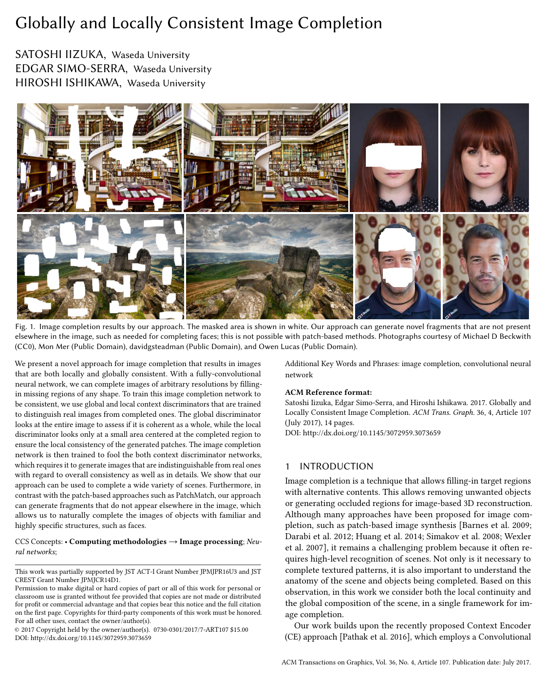
The experimental findings demonstrate significant performance advantages over existing methods. First, the dual-discriminator setup successfully generates entirely new image fragments—such as missing eyes, noses, or architectural elements—which patch-based tools cannot do. Second, in a blind user study evaluating the naturalness of completed facial images, participants perceived the generated faces as real 77% of the time, approaching the 96.5% baseline rating for authentic photographs. Third, the fully convolutional model processes images across arbitrary resolutions with high operational efficiency, completing large 1024x1024-pixel images in 0.56 seconds on a standard graphics processing unit, representing a roughly 15-fold speedup over central processing unit execution.

These results show that combining global scene comprehension with local texture validation resolves the trade-off between image sharpness and contextual logic. For organizations developing automated photo editing, visual restoration, or computer-generated graphics workflows, this approach reduces the labor needed for complex manual touch-ups and delivers consistent, production-ready outputs at interactive speeds without requiring per-image optimization.

To adopt and build on this technology, organizations should deploy GPU-accelerated pipelines for image repair tools and fine-tune specialized models on domain-specific datasets when dealing with recurring structured subjects like portraits or architectural assets. Further research and development should explore expanded network receptive fields to improve performance on large-scale hole extrapolation at image borders, where contextual cues are limited to a single side.

The primary operational limitations stem from fixed receptive field boundaries and structured semantics. While the network reliably repairs diverse textures and landscapes, it struggles with extremely large masks that exceed its spatial support and can fail on complex, heavily structured subjects, such as attempting to recreate partially occluded animals or human bodies against detailed backgrounds.

  • Paper: Generative Adversarial Networks, Ian J. Goodfellow et al. (2014). Reading the foundational Generative Adversarial Networks paper provides the essential adversarial loss framework built upon by the source article's global and local context discriminators.
  • Paper: Context Encoders: Feature Learning by Inpainting, Deepak Pathak et al. (2016). Understanding context encoders for unsupervised feature learning by inpainting establishes the primary baseline and task formulation that the source paper extends.
  • Paper: PatchMatch: a randomized correspondence algorithm for structural image editing, Connelly Barnes et al. (2009). Familiarity with the PatchMatch randomized correspondence algorithm clarifies the traditional patch-based methods that the source paper contrasts against and improves upon.
Cover for Globally and locally consistent image completion

Abstract

We present a novel approach for image completion that results in images that are both locally and globally consistent. With a fully-convolutional neural network, we can complete images of arbitrary resolutions by filling-in missing regions of any shape. To train this image completion network to be consistent, we use global and local context discriminators that are trained to distinguish real images from completed ones. The global discriminator looks at the entire image to assess if it is coherent as a whole, while the local discriminator looks only at a small area centered at the completed region to ensure the local consistency of the generated patches. The image completion network is then trained to fool the both context discriminator networks, which requires it to generate images that are indistinguishable from real ones with regard to overall consistency as well as in details. We show that our approach can be used to complete a wide variety of scenes. Furthermore, in contrast with the patch-based approaches such as PatchMatch, our approach can generate fragments that do not appear elsewhere in the image, which allows us to naturally complete the images of objects with familiar and highly specific structures, such as faces.

Table of Contents

  • 1 INTRODUCTION
  • 2 RELATED WORK
  • 3 APPROACH
  • 3.1 Convolutional Neural Networks
  • 3.2 Completion Network
  • 3.3 Context Discriminators
  • 3.4 Training
  • 3.5 Stable Training
  • 4 RESULTS
  • 4.1 Comparison with Existing Work
  • 4.2 Global and Local Consistency
  • 4.3 Effect of Post-Processing and Training Data
  • 4.4 Object Removal
  • 4.5 Faces and Facades
  • 4.6 User Study
  • 4.7 Additional Results
  • 4.8 Limitations and Discussion
  • 5 CONCLUSION
  • REFERENCES

Knowls

  1. Knowl 1 — Dual Context Discriminator Framework for Image Completion

    model/method

    The image completion framework consists of three deep neural networks: a fully convolutional completion network and two auxiliary context discriminators (a global discriminator and a local discriminator) used exclusively during training.

    • Completion Network (CC): A fully convolutional encoder-decoder network that takes an RGB image concatenated with a single-channel binary completion mask (where 11 indicates missing pixels to be completed and 00 indicates intact pixels). The network generates completed RGB values for the missing regions while retaining the original pixel values in unmasked regions.
    • Global Context Discriminator (DglobalD_{\text{global}}): Takes the full image rescaled to a fixed resolution (256×256256 \times 256 pixels) to assess global scene coherence, semantic plausibility, and structural consistency across the entire image.
    • Local Context Discriminator (DlocalD_{\text{local}}): Takes a high-resolution sub-image patch (128×128128 \times 128 pixels) centered directly on the completed region (or a random patch for uncorrupted real images) to evaluate local texture consistency, sharpness, and fine-grained visual details around the hole boundaries.

    Feature vectors produced by DglobalD_{\text{global}} and DlocalD_{\text{local}} are concatenated into a joint vector that is processed by a final fully-connected classification layer to predict the probability that the input image is authentic rather than synthetically completed. The completion network is trained adversarially to fool both discriminators simultaneously.

  2. Knowl 2 — Joint Reconstruction and Adversarial Inpainting Loss

    equation

    The image completion model is optimized using a joint objective function that combines a masked Mean Squared Error (MSE) reconstruction loss with a Generative Adversarial Network (GAN) loss:

    min⁡Cmax⁡DEx[L(x,Mc)+αlog⁡D(x,Md)+αlog⁡(1−D(C(x,Mc),Mc))]\min_{C} \max_{D} \mathbb{E}_{x} \left[ L(x, M_c) + \alpha \log D(x, M_d) + \alpha \log\left(1 - D(C(x, M_c), M_c)\right) \right]

    where the masked MSE loss L(x,Mc)L(x, M_c) is defined as:

    L(x,Mc)=∥Mc⊙(C(x,Mc)−x)∥2L(x, M_c) = \| M_c \odot (C(x, M_c) - x) \|^2

    Variable definitions and constraints:

    • x∈[0,1]H×W×3x \in [0, 1]^{H \times W \times 3} is the ground-truth input RGB image.
    • Mc∈{0,1}H×WM_c \in \{0, 1\}^{H \times W} is the binary completion mask, where Mc(u,v)=1M_c(u,v) = 1 denotes a missing pixel to be filled and Mc(u,v)=0M_c(u,v) = 0 denotes an intact pixel.
    • C(x,Mc)C(x, M_c) is the functional output of the completion network, which replaces missing pixels in xx with synthesized values while keeping non-masked pixels unchanged.
    • ⊙\odot represents the element-wise (Hadamard) product, and ∥⋅∥\|\cdot\| is the Euclidean norm (L2L_2 norm).
    • MdM_d is a randomly generated mask used to select arbitrary local patches from uncorrupted real training images for the discriminator.
    • D(⋅,⋅)∈[0,1]D(\cdot, \cdot) \in [0, 1] represents the unified context discriminator output (combining global and local discriminators) indicating the probability that an image is a real photograph rather than an output of CC.
    • α>0\alpha > 0 is a scalar hyperparameter weighting the adversarial loss relative to the MSE loss (set to α=0.0004\alpha = 0.0004).
  3. Knowl 3 — Completion Network Architecture with Dilated Convolutions

    model/method

    The completion network is a fully convolutional encoder-decoder architecture designed to process images of arbitrary spatial dimensions while preventing texture blurring:

    1. Input Preprocessing: The input is a 4-channel tensor formed by concatenating the RGB image (where the masked area is overwritten with the dataset mean pixel value) and the 1-channel binary mask (11 for masked pixels, 00 elsewhere).
    2. Downsampling (Encoder): The image resolution is reduced by a factor of 4 using strided convolutions (two downsamplings of stride 2×22 \times 2). The sequence is:
      • Convolution (5×55 \times 5 kernel, stride 1×11 \times 1, dilation η=1\eta = 1, 64 output channels)
      • Convolution (3×33 \times 3 kernel, stride 2×22 \times 2, dilation η=1\eta = 1, 128 output channels)
      • Convolution (3×33 \times 3 kernel, stride 1×11 \times 1, dilation η=1\eta = 1, 256 output channels)
      • Convolution (3×33 \times 3 kernel, stride 2×22 \times 2, dilation η=1\eta = 1, 256 output channels)
      • Convolution (3×33 \times 3 kernel, stride 1×11 \times 1, dilation η=1\eta = 1, 256 output channels)
    3. Context Expansion (Dilated Convolutions): In the mid-layers at 1/41/4 resolution, four dilated convolutional layers with 3×33 \times 3 kernels and 256 channels are applied with dilation factors η∈{2,4,8,16}\eta \in \{2, 4, 8, 16\}. The dilated convolution operation for layer inputs xx and outputs yy is:

    yu,v=σ(b+∑i=−kh′kh′∑j=−kw′kw′Wkh′+i,kw′+j xu+ηi,v+ηj)y_{u,v} = \sigma \left( b + \sum_{i=-k'_h}^{k'_h} \sum_{j=-k'_w}^{k'_w} W_{k'_h+i, k'_w+j} \, x_{u+\eta i, v+\eta j} \right)

    where kh′=(kh−1)/2k'_h = (k_h - 1)/2 and kw′=(kw−1)/2k'_w = (k_w - 1)/2. This series of dilated layers increases the spatial support (effective receptive field) of each output pixel to 303×303303 \times 303 pixels (compared to 95×9595 \times 95 pixels with standard convolutions), enabling the network to observe global image context outside large holes. 4. Upsampling (Decoder): Two deconvolutional layers with fractional stride 1/2×1/21/2 \times 1/2 restore the feature maps back to full input resolution:

    • Convolution (3×33 \times 3 kernel, stride 1×11 \times 1, dilation η=1\eta = 1, 256 output channels)
    • Convolution (3×33 \times 3 kernel, stride 1×11 \times 1, dilation η=1\eta = 1, 256 output channels)
    • Deconvolution (4×44 \times 4 kernel, stride 1/2×1/21/2 \times 1/2, dilation η=1\eta = 1, 128 output channels)
    • Convolution (3×33 \times 3 kernel, stride 1×11 \times 1, dilation η=1\eta = 1, 128 output channels)
    • Deconvolution (4×44 \times 4 kernel, stride 1/2×1/21/2 \times 1/2, dilation η=1\eta = 1, 64 output channels)
    • Convolution (3×33 \times 3 kernel, stride 1×11 \times 1, dilation η=1\eta = 1, 32 output channels)
    • Output Convolution (3×33 \times 3 kernel, stride 1×11 \times 1, dilation η=1\eta = 1, 3 output channels with sigmoid activation)

    All hidden layers use Rectified Linear Unit (ReLU) activations and Batch Normalization (which is merged into preceding convolutional layers at test time). Non-masked pixels outside the completion mask are reset to their original input RGB values.

  4. Knowl 4 — Global and Local Context Discriminators Architecture

    model/method

    The context discriminator network consists of two parallel convolutional branches followed by a fusion layer:

    1. Global Context Discriminator:
      • Input: Full image rescaled to 256×256×3256 \times 256 \times 3 pixels.
      • Layers: 6 successive convolutional layers, each using 5×55 \times 5 kernels and a stride of 2×22 \times 2, with output channel dimensions 64, 128, 256, 512, 512, and 512, followed by a fully connected layer producing a 1024-dimensional feature vector.
    2. Local Context Discriminator:
      • Input: 128×128×3128 \times 128 \times 3 pixel patch centered around the completed region (or a randomly sampled 128×128128 \times 128 patch for uncompleted real images).
      • Layers: 5 successive convolutional layers using 5×55 \times 5 kernels and a stride of 2×22 \times 2, with output channel dimensions 64, 128, 256, 512, and 512, followed by a fully connected layer producing a 1024-dimensional feature vector.
    3. Concatenation and Output Layer:
      • The 1024-dimensional outputs from both the global and local discriminators are concatenated into a single 2048-dimensional vector.
      • A single fully connected layer maps this 2048-dimensional representation to a scalar value, processed with a sigmoid activation function to output a continuous probability D(x,M)∈[0,1]D(x, M) \in [0, 1] indicating whether the image is real (11) or synthetic (00).
  5. Knowl 5 — Three-Phase Staged Adversarial Inpainting Training

    algorithm

    To overcome instability in adversarial learning, training is divided into three consecutive phases: completion network pretraining with MSE loss, discriminator pretraining from scratch, and joint adversarial fine-tuning.

    Input: Training images dataset, completion network CC, discriminator network DD, total iterations Ttrain=500,000T_{\text{train}} = 500{,}000, completion pretraining steps TC=90,000T_C = 90{,}000, discriminator pretraining steps TD=10,000T_D = 10{,}000, weighting parameter α=0.0004\alpha = 0.0004.
    Output: Trained completion network CC.
    for iteration t=1t = 1 to TtrainT_{\text{train}} do
        Sample minibatch of training images xx
        Generate random completion masks McM_c with hole sizes in range [96,128]×[96,128][96, 128] \times [96, 128]
        
        if t<TCt < T_C then
            # Phase 1: Pretrain completion network with MSE loss
            Update parameters θC\theta_C using ∇θC∥Mc⊙(C(x,Mc)−x)∥2\nabla_{\theta_C} \| M_c \odot (C(x, M_c) - x) \|^2
        else
            # Phase 2 & 3: Train discriminators
            Generate random patches/masks MdM_d for uncorrupted images
            Compute discriminator predictions D(x,Md)D(x, M_d) and D(C(x,Mc),Mc)D(C(x, M_c), M_c)
            Update parameters θD\theta_D using binary cross-entropy loss to maximize log⁡D(x,Md)+log⁡(1−D(C(x,Mc),Mc))\log D(x, M_d) + \log(1 - D(C(x, M_c), M_c))
            
            if t>TC+TDt > T_C + T_D then
                # Phase 3: Joint adversarial training
                Update parameters θC\theta_C using ∇θC(L(x,Mc)+αlog⁡(1−D(C(x,Mc),Mc)))\nabla_{\theta_C} \left( L(x, M_c) + \alpha \log(1 - D(C(x, M_c), M_c)) \right)
            end if
        end if
    end for

    All network parameters are updated using the ADADELTA optimization algorithm with batch size 96.

  6. Knowl 6 — Ablation Analysis of Global and Local Context Discriminators

    empirical result

    Ablation experiments comparing discriminator configurations reveal distinct, complementary roles for the global and local context discriminators:

    • Weighted MSE Only (No Discriminators): Fills missing regions with smooth, blurry pixel averages lacking high-frequency textures or details.
    • Weighted MSE + Global Discriminator Only: Preserves high-level semantic layout and scene consistency, but results in noticeable blurring and lack of realistic fine texture within the hole.
    • Weighted MSE + Local Discriminator Only: Synthesizes sharp, locally realistic high-frequency textures, but fails to maintain global scene structure, producing semantically inconsistent artifacts (such as disconnected objects or contradictory scene elements appearing in the completed hole).
    • Full Method (Global + Local Discriminators): The combination produces completions that are both locally sharp and globally coherent with the surrounding scene geometry and semantics.
  7. Knowl 7 — Boundary Blending Post-Processing via Fast Marching and Poisson Editing

    model/method

    To eliminate subtle color and illumination inconsistencies between generated pixels inside the hole and the surrounding original image, a post-processing pipeline is applied:

    1. The fast marching method is applied to compute an initial smooth boundary transition around the filled region.
    2. Poisson image blending is executed to solve Poisson differential equations over the target hole region using Dirichlet boundary conditions defined by the original unmasked image pixels.

    This blends the high-frequency semantic completions into the surrounding image while preserving the global color tone and illumination of the original photograph.

  8. Knowl 8 — CelebA Face Completion Naturalness User Study

    empirical result

    In a double-blind user study evaluating face completion naturalness on the CelebFaces Attributes (CelebA) validation set, 10 human participants were presented with either ground-truth photographs or completed images and asked to classify each image as real or synthetically modified.

    • Completed images produced by the model fine-tuned on CelebA were judged as real photographs 77.0% of the time (median score).
    • Ground-truth real photographs were correctly recognized as real 96.5% of the time.

    Unlike patch-based inpainting methods (such as PatchMatch) which can only copy and rearrange existing pixels from the input image and therefore fail when distinct facial features are occluded, the deep completion network generates entirely novel structural components (such as missing eyes, noses, or mouths) that match the identity, lighting, and pose of the face.

  9. Knowl 9 — Inference Computation Time Across Image Resolutions

    data/table

    The completion network execution time depends strictly on the total pixel resolution of the input image, rather than the shape or area of the missing hole. GPU acceleration yields a speedup of roughly 15×15\times to 16×16\times over multi-core CPU execution, achieving sub-second completions even on megapixel images.

    Image Size Pixels CPU (s) GPU (s) Speedup
    512×512512 \times 512 409,600 2.286 0.141 16.2×16.2\times
    768×768768 \times 768 589,824 4.933 0.312 15.8×15.8\times
    1024×10241024 \times 1024 1,048,576 8.262 0.561 14.7×14.7\times

    Measurements were conducted on an Intel Core i7-5960X CPU @ 3.00 GHz (8 cores) and an NVIDIA GeForce TITAN X GPU.

  10. Knowl 10 — Receptive Field and Image Extrapolation Limitations

    limitation

    The image completion model exhibits two primary structural failure modes:

    1. Spatial Support Bounds on Large Square Holes: The maximum spatial receptive field (spatial support) of the completion network is 303×303303 \times 303 pixels. Square missing regions with dimensions significantly exceeding this support cannot be filled realistically because pixels in the interior of the hole have no access to contextual information outside the hole. (Elongated or non-square masks with large areas can still be filled provided one dimension remains within the receptive field).
    2. Image Extrapolation and Boundary Masks: When the missing region lies on the outer boundary of the image (image extrapolation rather than inpainting/interpolation), context is available from only one side rather than surrounding the hole. This one-sided context frequently results in blurred, unnatural, or degenerate completions.

Coverage note — None was omitted; all key architectural components, mathematical loss formulations, training algorithms, empirical ablation findings, user study evaluations, runtime benchmarks, and limitations are fully covered.

References

  1. 1.Coloma Ballester, Marcelo Bertalmío, Vicent Caselles, Guillermo Sapiro, and Joan Verdera. 2001. Filling-in by joint interpolation of vector fields and gray levels. IEEE Transactions on Image Processing 10, 8 (2001), 1200–1211.
  2. 2.Connelly Barnes, Eli Shechtman, Adam Finkelstein, and Dan B Goldman. 2009. PatchMatch: A Randomized Correspondence Algorithm for Structural Image Editing. ACM Transactions on Graphics (Proceedings of SIGGRAPH) 28, 3 (2009), 24:1–24:11.
  3. 3.Connelly Barnes, Eli Shechtman, Dan B. Goldman, and Adam Finkelstein. 2010. The Generalized Patchmatch Correspondence Algorithm. In European Conference on Computer Vision. 29–43.
  4. 4.Marcelo Bertalmio, Guillermo Sapiro, Vincent Caselles, and Coloma Ballester. 2000. Image Inpainting. In ACM Transactions on Graphics (Proceedings of SIGGRAPH). 417–424.
  5. 5.M. Bertalmio, L. Vese, G. Sapiro, and S. Osher. 2003. Simultaneous structure and texture image inpainting. IEEE Transactions on Image Processing 12, 8 (2003), 882–889.
  6. 6.A. Criminisi, P. Perez, and K. Toyama. 2004. Region Filling and Object Removal by Exemplar-based Image Inpainting. IEEE Transactions on Image Processing 13, 9 (2004), 1200–1212.
  7. 7.Soheil Darabi, Eli Shechtman, Connelly Barnes, Dan B Goldman, and Pradeep Sen. 2012. Image Melding: Combining Inconsistent Images using Patch-based Synthesis. ACM Transactions on Graphics (Proceedings of SIGGRAPH) 31, 4, Article 82 (2012), 82:1–82:10 pages.
  8. 8.J. Deng, W. Dong, R. Socher, L.-J. Li, K. Li, and L. Fei-Fei. 2009. ImageNet: A Large-Scale Hierarchical Image Database. In CVPR09.
  9. 9.Yue Deng, Qionghai Dai, and Zengke Zhang. 2011. Graph Laplace for occluded face completion and recognition. IEEE Transactions on Image Processing 20, 8 (2011), 2329–2338.
  10. 10.Iddo Drori, Daniel Cohen-Or, and Hezy Yeshurun. 2003. Fragment-based Image Completion. ACM Transactions on Graphics (Proceedings of SIGGRAPH) 22, 3 (2003), 303–312.
  11. 11.Alexei Efros and Thomas Leung. 1999. Texture Synthesis by Non-parametric Sampling. In International Conference on Computer Vision. 1033–1038.
  12. 12.Alexei A. Efros and William T. Freeman. 2001. Image Quilting for Texture Synthesis and Transfer. In ACM Transactions on Graphics (Proceedings of SIGGRAPH). 341–346.
  13. 13.Kunihiko Fukushima. 1988. Neocognitron: A hierarchical neural network capable of visual pattern recognition. Neural networks 1, 2 (1988), 119–130.
  14. 14.Ian J. Goodfellow, Jean Pouget-Abadie, Mehdi Mirza, Bing Xu, David Warde-Farley, Sherjil Ozair, Aaron C. Courville, and Yoshua Bengio. 2014. Generative Adversarial Nets. In Conference on Neural Information Processing Systems. 2672–2680.
  15. 15.James Hays and Alexei A. Efros. 2007. Scene Completion Using Millions of Photographs. ACM Transactions on Graphics (Proceedings of SIGGRAPH) 26, 3, Article 4 (2007).
  16. 16.Kaiming He and Jian Sun. 2012. Statistics of Patch Offsets for Image Completion. In European Conference on Computer Vision. 16–29.
  17. 17.Jia-Bin Huang, Sing Bing Kang, Narendra Ahuja, and Johannes Kopf. 2014. Image Completion Using Planar Structure Guidance. ACM Transactions on Graphics (Proceedings of SIGGRAPH) 33, 4, Article 129 (2014), 10 pages.
  18. 18.Sergey Ioffe and Christian Szegedy. 2015. Batch Normalization: Accelerating Deep Network Training by Reducing Internal Covariate Shift. In International Conference on Machine Learning.
  19. 19.Phillip Isola, Jun-Yan Zhu, Tinghui Zhou, and Alexei A Efros. 2017. Image-to-Image Translation with Conditional Adversarial Networks. (2017).
  20. 20.Jiaya Jia and Chi-Keung Tang. 2003. Image repairing: robust image synthesis by adaptive ND tensor voting. In IEEE Conference on Computer Vision and Pattern Recognition, Vol. 1. 643–650.
  21. 21.Rolf Köhler, Christian Schuler, Bernhard Schölkopf, and Stefan Harmeling. 2014. Mask-specific inpainting with deep neural networks. In German Conference on Pattern Recognition.
  22. 22.Johannes Kopf, Wolf Kienzle, Steven Drucker, and Sing Bing Kang. 2012. Quality Prediction for Image Completion. ACM Transactions on Graphics (Proceedings of SIGGRAPH Asia) 31, 6, Article 131 (2012), 8 pages.
  23. 23.Vivek Kwatra, Irfan Essa, Aaron Bobick, and Nipun Kwatra. 2005. Texture Optimization for Example-based Synthesis. ACM Transactions on Graphics (Proceedings of SIGGRAPH) 24, 3 (July 2005), 795–802.
  24. 24.Vivek Kwatra, Arno Schödl, Irfan Essa, Greg Turk, and Aaron Bobick. 2003. Graphcut Textures: Image and Video Synthesis Using Graph Cuts. ACM Transactions on Graphics (Proceedings of SIGGRAPH) 22, 3 (July 2003), 277–286.
  25. 25.Yann LeCun, Bernhard Boser, John S Denker, Donnie Henderson, Richard E Howard, Wayne Hubbard, and Lawrence D Jackel. 1989. Backpropagation applied to handwritten zip code recognition. Neural computation 1, 4 (1989), 541–551.
  26. 26.Anat Levin, Assaf Zomet, and Yair Weiss. 2003. Learning How to Inpaint from Global Image Statistics. In International Conference on Computer Vision. 305–312.
  27. 27.Rongjian Li, Wenlu Zhang, Heung-Il Suk, Li Wang, Jiang Li, Dinggang Shen, and Shuiwang Ji. 2014. Deep learning based imaging data completion for improved brain disease diagnosis. In International Conference on Medical Image Computing and Computer-Assisted Intervention. Springer, 305–312.
  28. 28.Ziwei Liu, Ping Luo, Xiaogang Wang, and Xiaoou Tang. 2015. Deep Learning Face Attributes in the Wild. In International Conference on Computer Vision.
  29. 29.Jonathan Long, Evan Shelhamer, and Trevor Darrell. 2015. Fully convolutional networks for semantic segmentation. In IEEE Conference on Computer Vision and Pattern Recognition.
  30. 30.Umar Mohammed, Simon JD Prince, and Jan Kautz. 2009. Visio-lization: generating novel facial images. ACM Transactions on Graphics (Proceedings of SIGGRAPH) 28, 3 (2009), 57.
  31. 31.Vinod Nair and Geoffrey E Hinton. 2010. Rectified linear units improve restricted boltzmann machines. In International Conference on Machine Learning. 807–814.
  32. 32.Deepak Pathak, Philipp Krähenbühl, Jeff Donahue, Trevor Darrell, and Alexei Efros. 2016. Context Encoders: Feature Learning by Inpainting. In IEEE Conference on Computer Vision and Pattern Recognition.
  33. 33.Darko Pavić, Volker Schönefeld, and Leif Kobbelt. 2006. Interactive image completion with perspective correction. The Visual Computer 22, 9 (2006), 671–681.
  34. 34.Patrick Pérez, Michel Gangnet, and Andrew Blake. 2003. Poisson Image Editing. ACM Transactions on Graphics (Proceedings of SIGGRAPH) 22, 3 (July 2003), 313–318.
  35. 35.Alec Radford, Luke Metz, and Soumith Chintala. 2016. Unsupervised Representation Learning with Deep Convolutional Generative Adversarial Networks. In International Conference on Learning Representations.
  36. 36.Radim Šára Radim Tyleček. 2013. Spatial Pattern Templates for Recognition of Objects with Regular Structure. In German Conference on Pattern Recognition. Saarbrucken, Germany.
  37. 37.Jimmy SJ Ren, Li Xu, Qiong Yan, and Wenxiu Sun. 2015. Shepard Convolutional Neural Networks. In Conference on Neural Information Processing Systems.
  38. 38.D.E. Rumelhart, G.E. Hinton, and R.J. Williams. 1986. Learning representations by back-propagating errors. In Nature.
  39. 39.Tim Salimans, Ian Goodfellow, Wojciech Zaremba, Vicki Cheung, Alec Radford, and Xi Chen. 2016. Improved techniques for training gans. In Conference on Neural Information Processing Systems.
  40. 40.Denis Simakov, Yaron Caspi, Eli Shechtman, and Michal Irani. 2008. Summarizing visual data using bidirectional similarity. In IEEE Conference on Computer Vision and Pattern Recognition. 1–8.
  41. 41.Jian Sun, Lu Yuan, Jiaya Jia, and Heung-Yeung Shum. 2005. Image Completion with Structure Propagation. ACM Transactions on Graphics (Proceedings of SIGGRAPH) 24, 3 (July 2005), 861–868. DOI:https://doi.org/10.1145/1073204.1073274
  42. 42.Alexandru Telea. 2004. An Image Inpainting Technique Based on the Fast Marching Method. Journal of Graphics Tools 9, 1 (2004), 23–34.
  43. 43.Yonatan Wexler, Eli Shechtman, and Michal Irani. 2007. Space-Time Completion of Video. IEEE Transactions on Pattern Analysis and Machine Intelligence 29, 3 (2007), 463–476.
  44. 44.Oliver Whyte, Josef Sivic, and Andrew Zisserman. 2009. Get Out of my Picture! Internet-based Inpainting. In British Machine Vision Conference.
  45. 45.Junyuan Xie, Linli Xu, and Enhong Chen. 2012. Image Denoising and Inpainting with Deep Neural Networks. In Conference on Neural Information Processing Systems. 341–349.
  46. 46.Chao Yang, Xin Lu, Zhe Lin, Eli Shechtman, Oliver Wang, and Hao Li. 2017. High-Resolution Image Inpainting using Multi-Scale Neural Patch Synthesis. In IEEE Conference on Computer Vision and Pattern Recognition.
  47. 47.Fisher Yu and Vladlen Koltun. 2016. Multi-Scale Context Aggregation by Dilated Convolutions. In International Conference on Learning Representations.
  48. 48.Matthew D. Zeiler. 2012. ADADELTA: An Adaptive Learning Rate Method. CoRR abs/1212.5701 (2012).
  49. 49.Bolei Zhou, Aditya Khosla, Àgata Lapedriza, Antonio Torralba, and Aude Oliva. 2016. Places: An Image Database for Deep Scene Understanding. CoRR abs/1610.02055 (2016).

Citation

MLA
Iizuka, S., et al. “Globally and Locally Consistent Image Completion”. ACM Transactions on Graphics, vol. 36, no. 4, 2017, pp. 1–4, https://doi.org/10.1145/3072959.3073659.
APA
Iizuka, S., Simo-Serra, E., & Ishikawa, H. (2017). Globally and locally consistent image completion. ACM Transactions on Graphics, 36(4), 1–14. https://doi.org/10.1145/3072959.3073659
Chicago
Iizuka, S., E. Simo-Serra, and H. Ishikawa. 2017. “Globally and Locally Consistent Image Completion”. ACM Transactions on Graphics 36 (4): 1–14. https://doi.org/10.1145/3072959.3073659.
Harvard
Iizuka, S., Simo-Serra, E. and Ishikawa, H. (2017) “Globally and locally consistent image completion”, ACM Transactions on Graphics, 36(4), pp. 1–14. Available at: https://doi.org/10.1145/3072959.3073659.
Vancouver
1. Iizuka S, Simo-Serra E, Ishikawa H (2017) Globally and locally consistent image completion. ACM Transactions on Graphics 36:1–14

BibTeX

@article{Iizuka_2017, title={Globally and locally consistent image completion}, volume={36}, ISSN={1557-7368}, url={http://dx.doi.org/10.1145/3072959.3073659}, DOI={10.1145/3072959.3073659}, number={4}, journal={ACM Transactions on Graphics}, publisher={Association for Computing Machinery (ACM)}, author={Iizuka, Satoshi and Simo-Serra, Edgar and Ishikawa, Hiroshi}, year={2017}, month=July, pages={1–14} }
Metadata:Crossref

Source Code

This paper has an official code repository available. Click below to access the source code.

View Repository

Access the Paper

This paper is available from its original source. Click below to access the PDF.

Open PDF