Matryoshka Representation Learning

Aditya Kusupati $^{\dagger\diamond,}$, Gantavya Bhatt$^{\dagger}$, Aniket Rege$^{*\dagger}$
Matthew Wallingford$^{\dagger}$, Aditya Sinha$^{\diamond}$, Vivek Ramanujan$^{\dagger}$, William Howard-Snyder$^{\dagger}$
Kaifeng Chen$^{\diamond}$, Sham Kakade$^{\ddagger}$, Prateek Jain$^{\diamond}$ and Ali Farhadi$^{\dagger}$
kusupati,[email protected], [email protected]

$^{\dagger}$ University of Washington, $^{\diamond}$ Google Research, $^{\ddagger}$ Harvard University

$^{*}$ Equal contribution -- AK led the project with extensive support from GB and AR for experimentation.

Abstract

Learned representations are a central component in modern ML systems, serving a multitude of downstream tasks. When training such representations, it is often the case that computational and statistical constraints for each downstream task are unknown. In this context, rigid fixed-capacity representations can be either over or under-accommodating to the task at hand. This leads us to ask: can we design a flexible representation that can adapt to multiple downstream tasks with varying computational resources? Our main contribution is ${\rm MatryoshkaRepresentationLearning}$ (${\rm MRL}$) which encodes information at different granularities and allows a single embedding to adapt to the computational constraints of downstream tasks. ${\rm MRL}$ minimally modifies existing representation learning pipelines and imposes no additional cost during inference and deployment. ${\rm MRL}$ learns coarse-to-fine representations that are at least as accurate and rich as independently trained low-dimensional representations. The flexibility within the learned ${\rm Matryoshka~Representations}$ offer: (a) up to $\mathbf{14}\times$ smaller embedding size for ImageNet-1K classification at the same level of accuracy; (b) up to $\mathbf{14}\times$ real-world speed-ups for large-scale retrieval on ImageNet-1K and 4K; and (c) up to $\mathbf{2}$ % accuracy improvements for long-tail few-shot classification, all while being as robust as the original representations. Finally, we show that ${\rm MRL}$ extends seamlessly to web-scale datasets (ImageNet, JFT) across various modalities – vision (ViT, ResNet), vision + language (ALIGN) and language (BERT). ${\rm MRL}$ code and pretrained models are open-sourced at https://github.com/RAIVNLab/MRL.

Executive Summary: Modern machine learning systems rely on learned representations—compact encodings of data like images or text—that power tasks such as classification and search. However, these representations are typically fixed in size, creating challenges at scale. As data volumes grow to billions of items, the computational cost of processing high-dimensional embeddings surges, especially for tasks with varying resource demands. Fixed representations either waste resources on simple tasks or underperform on complex ones, limiting efficiency in real-world applications like web-scale search or image retrieval.

This work introduces Matryoshka Representation Learning (MRL), a method to create flexible representations that adapt to different computational budgets. The goal was to train a single high-dimensional embedding that contains nested, lower-dimensional versions, each optimized for accuracy like an independently trained model, without extra inference costs.

The approach modifies standard representation learning pipelines minimally. Researchers trained models to optimize losses at a small set of nested dimensions, roughly logarithmically spaced (e.g., 8, 16, up to 2048 for image models), within the full vector. They tested this on supervised vision models like ResNet on ImageNet (1.3 million images), self-supervised models like Vision Transformers on JFT-300M (300 million images), vision-language models like ALIGN on 1.8 billion image-text pairs, and language models like BERT on text corpora. Baselines included fixed-size models, post-training compression, and multi-network ensembles, evaluated over months on GPU clusters for credibility, using standard metrics like classification accuracy and retrieval precision.

Key findings highlight MRL's advantages. First, MRL embeddings match or exceed the accuracy of separately trained low-dimensional models; for example, an 8-dimensional MRL slice achieved 66.6% accuracy on ImageNet classification, compared to 65.3% for a dedicated model, while information interpolates smoothly across unoptimized sizes. Second, in adaptive classification—routing easy examples to low dimensions and hard ones to high—MRL delivered 76.3% accuracy using an average of just 37 dimensions, about 14 times fewer than the 512 needed by baselines for similar performance. Third, for retrieval on ImageNet, MRL enabled shortlisting candidates with low dimensions (e.g., 16) and reranking with high ones, matching full 2048-dimensional accuracy but with 128 times fewer floating-point operations and 14 times faster wall-clock time. Fourth, MRL improved long-tail few-shot learning by up to 2% on novel classes, likely due to better semantic sharing across dimensions. Fifth, it scaled seamlessly to web-scale data and modalities, with gains in robustness on out-of-distribution tests like ImageNet variants.

These results mean MRL addresses a core inefficiency in ML deployment: rigid embeddings drive up costs in memory, processing, and storage for large databases, often bottlenecking systems beyond the initial model training. By packing coarse-to-fine information into one vector, MRL cuts these costs while maintaining or boosting performance, differing from prior compression methods that lose accuracy at low dimensions. This matters for cost savings—potentially millions in cloud compute for search engines—and enables adaptive systems that adjust to device constraints or task difficulty, improving safety in varied environments without retraining multiple models.

Next, organizations should integrate MRL into existing pipelines for classification and retrieval tasks, starting with finetuning pretrained models to induce nesting (achieving near full benefits with modest compute). For retrieval, implement adaptive shortlisting and funnel reranking to realize speedups; trade-offs include slight added complexity in routing logic versus baselines. Further work is needed: pilot on proprietary datasets to tune loss weights for specific tasks, and combine with approximate search tools for ultra-scale. Before full rollout, validate on diverse real-world scenarios.

Limitations include reliance on logarithmic dimension spacing, which assumes saturation patterns hold across datasets—uniform spacing underperforms at low sizes. Finetuning from non-MRL models induces nesting but lags end-to-end training by 5-6% at tiny dimensions. Confidence is high on benchmarks (e.g., consistent gains across 1,000+ classes), but caution applies to highly skewed or adversarial data, where routing policies may need refinement.

1. Introduction

Section Summary: Learned representations in machine learning systems are like compact summaries of data that are computed once and reused for various tasks, but using them at massive scales becomes costly because they are fixed in size and don't adapt to different needs. Traditional approaches to make these representations more flexible, such as training multiple models or compressing them, often involve high overhead or reduced accuracy. Matryoshka Representation Learning introduces a clever solution by training a single high-dimensional representation where smaller nested subsets act like accurate lower-dimensional versions, enabling efficient, adaptive use in tasks like image classification and search without extra computation during deployment.

Learned representations ([1]) are fundamental building blocks of real-world ML systems ([2, 3]). Trained once and frozen, $d$-dimensional representations encode rich information and can be used to perform multiple downstream tasks ([4]). The deployment of deep representations has two steps: (1) an expensive yet constant-cost forward pass to compute the representation ([5]) and (2) utilization of the representation for downstream applications ([6, 7]). Compute costs for the latter part of the pipeline scale with the embedding dimensionality as well as the data size ($N$) and label space ($L$). At web-scale ([8, 9]) this utilization cost overshadows the feature computation cost. The rigidity in these representations forces the use of high-dimensional embedding vectors across multiple tasks despite the varying resource and accuracy constraints that require flexibility.

Human perception of the natural world has a naturally coarse-to-fine granularity ([10, 11]). However, perhaps due to the inductive bias of gradient-based training ([12]), deep learning models tend to diffuse "information" across the entire representation vector. The desired elasticity is usually enabled in the existing flat and fixed representations either through training multiple low-dimensional models ([5]), jointly optimizing sub-networks of varying capacity ([13, 14]) or post-hoc compression ([15, 16]). Each of these techniques struggle to meet the requirements for adaptive large-scale deployment either due to training/maintenance overhead, numerous expensive forward passes through all of the data, storage and memory cost for multiple copies of encoded data, expensive on-the-fly feature selection or a significant drop in accuracy. By encoding coarse-to-fine-grained representations, which are as accurate as the independently trained counterparts, we learn with minimal overhead a representation that can be deployed adaptively at no additional cost during inference.

We introduce ${\rm MatryoshkaRepresentationLearning}$ (${\rm MRL}$) to induce flexibility in the learned representation. ${\rm MRL}$ learns representations of varying capacities within the same high-dimensional vector through explicit optimization of $O(\log(d))$ lower-dimensional vectors in a nested fashion, hence the name ${\rm Matryoshka}$. ${\rm MRL}$ can be adapted to any existing representation pipeline and is easily extended to many standard tasks in computer vision and natural language processing. Figure 1 illustrates the core idea of ${\rm MatryoshkaRepresentationLearning}$ (${\rm MRL}$) and the adaptive deployment settings of the learned ${\rm Matryoshka~Representations}$.

:::: {cols="1"}

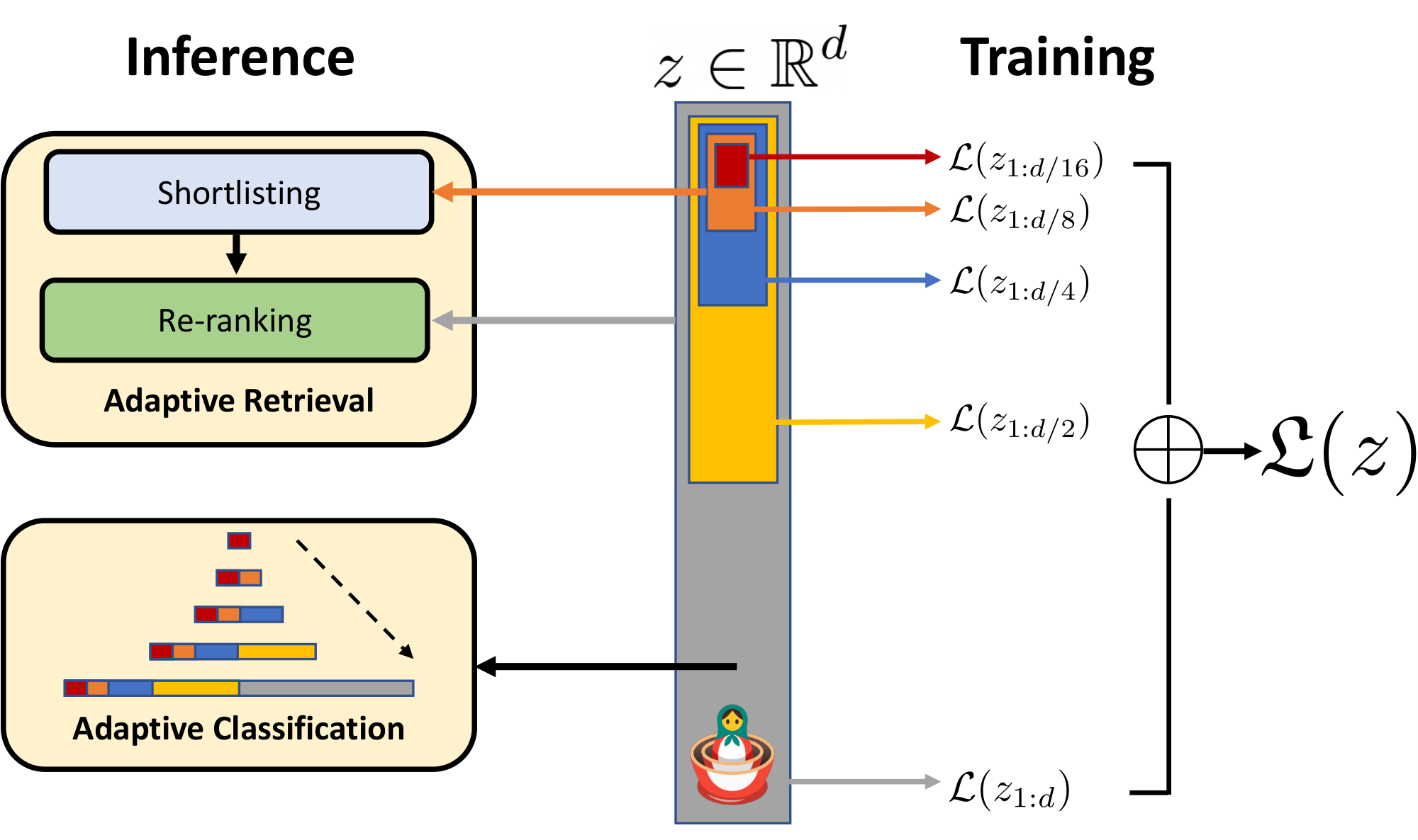
Figure 1: ${\rm MatryoshkaRepresentationLearning}$ is adaptable to any representation learning setup and begets a ${\rm MatryoshkaRepresentation}$ $z$ by optimizing the original loss $\mathcal{L}(.)$ at $O(\log(d))$ chosen representation sizes. ${\rm MatryoshkaRepresentation}$ can be utilized effectively for adaptive deployment across environments and downstream tasks. ::::

The first $m$-dimensions, $m\in[d]$, of the ${\rm MatryoshkaRepresentation}$ is an information-rich low-dimensional vector, at no additional training cost, that is as accurate as an independently trained $m$-dimensional representation. The information within the ${\rm MatryoshkaRepresentation}$ increases with the dimensionality creating a coarse-to-fine grained representation, all without significant training or additional deployment overhead. ${\rm MRL}$ equips the representation vector with the desired flexibility and multifidelity that can ensure a near-optimal accuracy-vs-compute trade-off. With these advantages, ${\rm MRL}$ enables adaptive deployment based on accuracy and compute constraints.

The ${\rm MatryoshkaRepresentations}$ improve efficiency for large-scale classification and retrieval without any significant loss of accuracy. While there are potentially several applications of coarse-to-fine ${\rm MatryoshkaRepresentations}$, in this work we focus on two key building blocks of real-world ML systems: large-scale classification and retrieval. For classification, we use adaptive cascades with the variable-size representations from a model trained with ${\rm MRL}$, significantly reducing the average dimension of embeddings needed to achieve a particular accuracy. For example, on ImageNet-1K, ${\rm MRL}$ + adaptive classification results in up to a $14\times$ smaller representation size at the same accuracy as baselines (Section 4.2.1). Similarly, we use ${\rm MRL}$ in an adaptive retrieval system. Given a query, we shortlist retrieval candidates using the first few dimensions of the query embedding, and then successively use more dimensions to re-rank the retrieved set. A simple implementation of this approach leads to $128\times$ theoretical (in terms of FLOPS) and $14\times$ wall-clock time speedups compared to a single-shot retrieval system that uses a standard embedding vector; note that ${\rm MRL}$ 's retrieval accuracy is comparable to that of single-shot retrieval (Section 4.3.1). Finally, as ${\rm MRL}$ explicitly learns coarse-to-fine representation vectors, intuitively it should share more semantic information among its various dimensions (Figure 8). This is reflected in up to $2%$ accuracy gains in long-tail continual learning settings while being as robust as the original embeddings. Furthermore, due to its coarse-to-fine grained nature, ${\rm MRL}$ can also be used as method to analyze hardness of classification among instances and information bottlenecks.

We make the following key contributions:

1. We introduce ${\rm MatryoshkaRepresentationLearning}$ (${\rm MRL}$) to obtain flexible representations (${\rm Matryoshka~Representations}$) for adaptive deployment (Section 3).
2. Up to $14\times$ faster yet accurate large-scale classification and retrieval using ${\rm MRL}$ (Section 4).
3. Seamless adaptation of ${\rm MRL}$ across modalities (vision - ResNet & ViT, vision + language - ALIGN, language - BERT) and to web-scale data (ImageNet-1K/4K, JFT-300M and ALIGN data).
4. Further analysis of ${\rm MRL}$ 's representations in the context of other downstream tasks (Section 5).

2. Related Work

Section Summary: Researchers have developed versatile representations for images and text using massive datasets through methods like supervised training or self-supervised tasks such as predicting missing words or reconstructing data, which power advanced models for vision and language. To make classification and retrieval more efficient, especially with growing data sizes and complex searches, techniques like approximate nearest neighbor searches, dimensionality reduction, and hierarchical structures help reduce computational demands without losing too much accuracy. The proposed Matryoshka Representation Learning (MRL) builds on these by creating nested, adaptable representations within a single model that maintain high accuracy at various sizes, avoiding the need for multiple processing runs and enabling scalable applications.

Representation Learning.

Large-scale datasets like ImageNet ([17, 18]) and JFT ([9]) enabled the learning of general purpose representations for computer vision ([4, 19]). These representations are typically learned through supervised and un/self-supervised learning paradigms. Supervised pretraining ([5, 20, 21]) casts representation learning as a multi-class/label classification problem, while un/self-supervised learning learns representation via proxy tasks like instance classification ([22]) and reconstruction ([23, 24]). Recent advances ([25, 26]) in contrastive learning ([27]) enabled learning from web-scale data ([28]) that powers large-capacity cross-modal models ([29, 30, 31, 32]). Similarly, natural language applications are built ([33]) on large language models ([34]) that are pretrained ([35, 36]) in a un/self-supervised fashion with masked language modelling ([37]) or autoregressive training ([38]).

${\rm MatryoshkaRepresentationLearning}$ (${\rm MRL}$) is complementary to all these setups and can be adapted with minimal overhead (Section 3). ${\rm MRL}$ equips representations with multifidelity at no additional cost which enables adaptive deployment based on the data and task (Section 4).

Efficient Classification and Retrieval.

Efficiency in classification and retrieval during inference can be studied with respect to the high yet constant deep featurization costs or the search cost which scales with the size of the label space and data. Efficient neural networks address the first issue through a variety of algorithms ([39, 40]) and design choices ([41, 42, 43]). However, with a strong featurizer, most of the issues with scale are due to the linear dependence on number of labels ($L$), size of the data ($N$) and representation size ($d$), stressing RAM, disk and processor all at the same time.

The sub-linear complexity dependence on number of labels has been well studied in context of compute ([44, 45, 46]) and memory ([47]) using Approximate Nearest Neighbor Search (ANNS) ([48]) or leveraging the underlying hierarchy ([49, 50]). In case of the representation size, often dimensionality reduction ([51, 52]), hashing techniques ([53, 54, 55]) and feature selection ([56]) help in alleviating selective aspects of the $O(d)$ scaling at a cost of significant drops in accuracy. Lastly, most real-world search systems ([57, 8]) are often powered by large-scale embedding based retrieval ([58, 2]) that scales in cost with the ever increasing web-data. While categorization ([7, 59]) clusters similar things together, it is imperative to be equipped with retrieval capabilities that can bring forward every instance ([60]). Approximate Nearest Neighbor Search (ANNS) ([61]) makes it feasible with efficient indexing ([53]) and traversal ([62, 63]) to present the users with the most similar documents/images from the database for a requested query. Widely adopted HNSW ([48]) ($O(d\log(N))$) is as accurate as exact retrieval ($O(dN)$) at the cost of a graph-based index overhead for RAM and disk ([64]).

${\rm MRL}$ tackles the linear dependence on embedding size, $d$, by learning multifidelity ${\rm MatryoshkaRepresentations}$. Lower-dimensional ${\rm MatryoshkaRepresentations}$ are as accurate as independently trained counterparts without the multiple expensive forward passes. ${\rm MatryoshkaRepresentations}$ provide an intermediate abstraction between high-dimensional vectors and their efficient ANNS indices through the adaptive embeddings nested within the original representation vector (Section 4). All other aforementioned efficiency techniques are complementary and can be readily applied to the learned ${\rm MatryoshkaRepresentations}$ obtained from ${\rm MRL}$.

Several works in efficient neural network literature ([13, 65, 14]) aim at packing neural networks of varying capacity within the same larger network. However, the weights for each progressively smaller network can be different and often require distinct forward passes to isolate the final representations. This is detrimental for adaptive inference due to the need for re-encoding the entire retrieval database with expensive sub-net forward passes of varying capacities. Several works ([66, 67, 68, 69]) investigate the notions of intrinsic dimensionality and redundancy of representations and objective spaces pointing to minimum description length ([70]). Finally, ordered representations proposed by [71] use nested dropout in the context of autoencoders to learn nested representations. ${\rm MRL}$ differentiates itself in formulation by optimizing only for $O(\log(d))$ nesting dimensions instead of $O(d)$. Despite this, ${\rm MRL}$ diffuses information to intermediate dimensions interpolating between the optimized ${\rm Matryoshka~Representation}$ sizes accurately (Figure 8); making web-scale feasible.

3. ${\rm MatryoshkaRepresentationLearning}$

Section Summary: Matryoshka Representation Learning, or MRL, is a method for training neural networks to produce a single high-dimensional vector that represents data in a flexible, nested way, similar to Russian dolls where smaller versions inside can still capture key information independently. For each chosen size in a small set of dimensions, like powers of two up to the full size, the method trains separate classifiers on just the first few parts of the vector to ensure they work well for tasks like image classification, all optimized together with equal weighting. This approach is efficient, adaptable to other learning setups like language modeling or contrastive learning, and even produces useful representations for sizes between the chosen ones without extra training.

For $d\in\mathbb{N}$, consider a set $\mathcal{M}\subset [d]$ of representation sizes. For a datapoint $x$ in the input domain $\mathcal{X}$, our goal is to learn a $d$-dimensional representation vector $z \in \mathbb{R}^d$. For every $m\in\mathcal{M}$, ${\rm MatryoshkaRepresentationLearning}$ (${\rm MRL}$) enables each of the first $m$ dimensions of the embedding vector, $z_{1:m}\in\mathbb{R}^m$ to be independently capable of being a transferable and general purpose representation of the datapoint $x$. We obtain $z$ using a deep neural network $F(, \cdot, ;\theta_F)\colon \mathcal{X} \rightarrow \mathbb{R}^d$ parameterized by learnable weights $\theta_F$, i.e., $z \coloneqq F(x; \theta_F)$. The multi-granularity is captured through the set of the chosen dimensions $\mathcal{M}$, that contains less than $\log(d)$ elements, i.e., $\lvert \mathcal{M}\rvert \leq \left\lfloor\log(d)\right\rfloor$. The usual set $\mathcal{M}$ consists of consistent halving until the representation size hits a low information bottleneck. We discuss the design choices in Section 4 for each of the representation learning settings.

For the ease of exposition, we present the formulation for fully supervised representation learning via multi-class classification. ${\rm MatryoshkaRepresentationLearning}$ modifies the typical setting to become a multi-scale representation learning problem on the same task. For example, we train ResNet50 ([5]) on ImageNet-1K ([18]) which embeds a $224 \times 224$ pixel image into a $d=2048$ representation vector and then passed through a linear classifier to make a prediction, $\hat{y}$ among the $L=1000$ labels. For ${\rm MRL}$, we choose $\mathcal{M} = {8, 16, \ldots, 1024, 2048}$ as the nesting dimensions.

Suppose we are given a labelled dataset $\mathcal{D}={(x_1, y_1), \ldots, (x_N, y_N)}$ where $x_i\in \mathcal{X}$ is an input point and $y_i \in [L]$ is the label of $x_i$ for all $i\in[N]$. ${\rm MRL}$ optimizes the multi-class classification loss for each of the nested dimension $m\in \mathcal{M}$ using standard empirical risk minimization using a separate linear classifier, parameterized by $\mathbf{W}^{(m)} \in \mathbb{R}^{L\times m}$. All the losses are aggregated after scaling with their relative importance $\left(c_m \geq 0\right)_{m\in\mathcal{M}}$ respectively. That is, we solve

$ \min_{\left\lbrace\mathbf{W}^{(m)}\right\rbrace_{m\in\mathcal{M}}, \ \theta_F} \frac{1}{N}\sum_{i\in [N]} \sum_{m\in \mathcal{M}} c_m\cdot{\cal L}\left(\mathbf{W}^{(m)} \cdot F(x_i; \theta_F)_{1:m}\ ;\ y_i\right) ,\tag{1} $

where ${\cal L}\colon \mathbb{R}^L\times [L] \to \mathbb{R}_+$ is the multi-class softmax cross-entropy loss function. This is a standard optimization problem that can be solved using sub-gradient descent methods. We set all the importance scales, $c_m=1$ for all $m\in\mathcal{M}$; see Section 5 for ablations. Lastly, despite only optimizing for $O(\log(d))$ nested dimensions, ${\rm MRL}$ results in accurate representations, that interpolate, for dimensions that fall between the chosen granularity of the representations (Section 4.2).

We call this formulation as ${\rm MatryoshkaRepresentationLearning}$ (${\rm MRL}$). A natural way to make this efficient is through weight-tying across all the linear classifiers, i.e., by defining $\mathbf{W}^{(m)} = \mathbf{W}_{1:m}$ for a set of common weights $\mathbf{W}\in\mathbb{R}^{L\times d}$. This would reduce the memory cost due to the linear classifiers by almost half, which would be crucial in cases of extremely large output spaces ([7, 59]). This variant is called Efficient ${\rm MatryoshkaRepresentationLearning}$ (MRL–E). Refer to Algorithm 1 and Algorithm 2 in Appendix A for the building blocks of ${\rm MatryoshkaRepresentationLearning}$ (${\rm MRL}$).

Adaptation to Learning Frameworks.

${\rm MRL}$ can be adapted seamlessly to most representation learning frameworks at web-scale with minimal modifications (Section 4.1). For example, ${\rm MRL}$ 's adaptation to masked language modelling reduces to MRL–E due to the weight-tying between the input embedding matrix and the linear classifier. For contrastive learning, both in context of vision & vision + language, ${\rm MRL}$ is applied to both the embeddings that are being contrasted with each other. The presence of normalization on the representation needs to be handled independently for each of the nesting dimension for best results (see Appendix C for more details).

4. Applications

Section Summary: This section explores the use of Matryoshka Representation Learning (MRL), a method for creating flexible, nested data representations, across various tasks like image classification, vision-language matching, and language modeling on large datasets. It evaluates these representations through accuracy tests, showing that MRL matches or exceeds traditional fixed-size models, especially at smaller dimensions, and scales well to massive web-scale data without needing separate training for each size. The learned representations enable practical downstream uses, such as adaptive classification and retrieval, allowing efficient deployment by adjusting detail levels as needed.

In this section, we discuss ${\rm MatryoshkaRepresentationLearning}$ (${\rm MRL}$) for a diverse set of applications along with an extensive evaluation of the learned multifidelity representations. Further, we showcase the downstream applications of the learned ${\rm Matryoshka~Representations}$ for flexible large-scale deployment through (a) Adaptive Classification (AC) and (b) Adaptive Retrieval (AR).

4.1 Representation Learning

We adapt ${\rm MatryoshkaRepresentationLearning}$ (${\rm MRL}$) to various representation learning setups (a) Supervised learning for vision: ResNet50 ([5]) on ImageNet-1K ([18]) and ViT-B/16 ([72]) on JFT-300M ([9]), (b) Contrastive learning for vision + language: ALIGN model with ViT-B/16 vision encoder and BERT language encoder on ALIGN data ([30]) and (c) Masked language modelling: BERT ([37]) on English Wikipedia and BooksCorpus ([73]). Please refer to Appendix B and Appendix C for details regarding the model architectures, datasets and training specifics.

We do not search for best hyper-parameters for all ${\rm MRL}$ experiments but use the same hyper-parameters as the independently trained baselines. ResNet50 outputs a $2048$-dimensional representation while ViT-B/16 and BERT-Base output $768$-dimensional embeddings for each data point. We use $\mathcal{M} = {8, 16, 32, 64, 128, 256, 512, 1024, 2048}$ and $\mathcal{M} = {12, 24, 48, 96, 192, 384, 768}$ as the explicitly optimized nested dimensions respectively. Lastly, we extensively compare the ${\rm MRL}$ and MRL–E models to independently trained low-dimensional (fixed feature) representations (FF), dimensionality reduction (SVD), sub-net method (slimmable networks ([14])) and randomly selected features of the highest capacity FF model.

In Section 4.2, we evaluate the quality and capacity of the learned representations through linear classification/probe (LP) and 1-nearest neighbour (1-NN) accuracy. Experiments show that ${\rm MRL}$ models remove the dependence on $|\mathcal{M}|$ resource-intensive independently trained models for the coarse-to-fine representations while being as accurate. Lastly, we show that despite optimizing only for $|\mathcal{M}|$ dimensions, ${\rm MRL}$ models diffuse the information, in an interpolative fashion, across all the $d$ dimensions providing the finest granularity required for adaptive deployment.

4.2 Classification

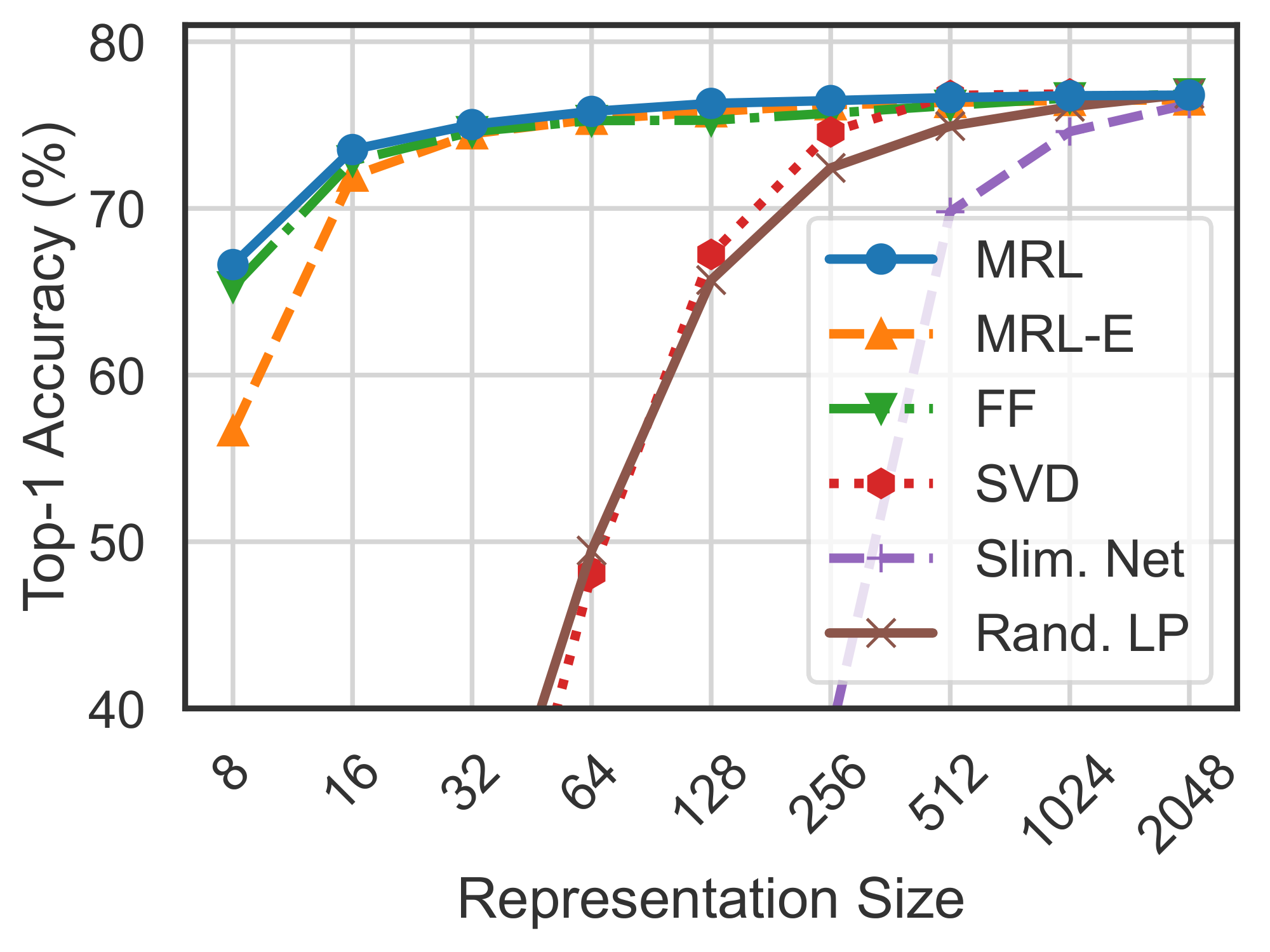
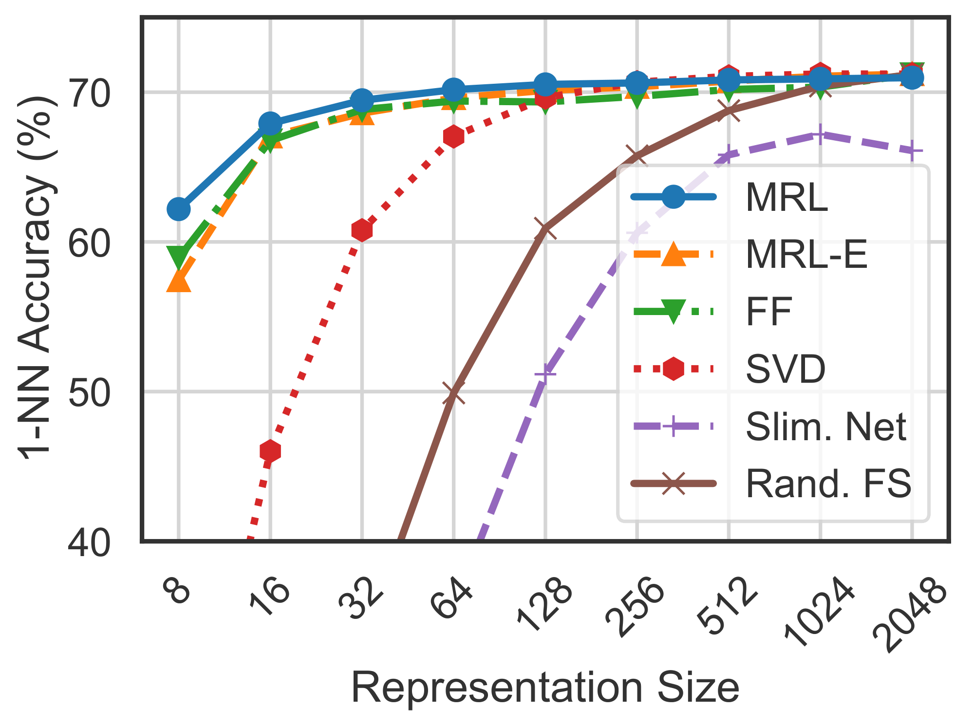
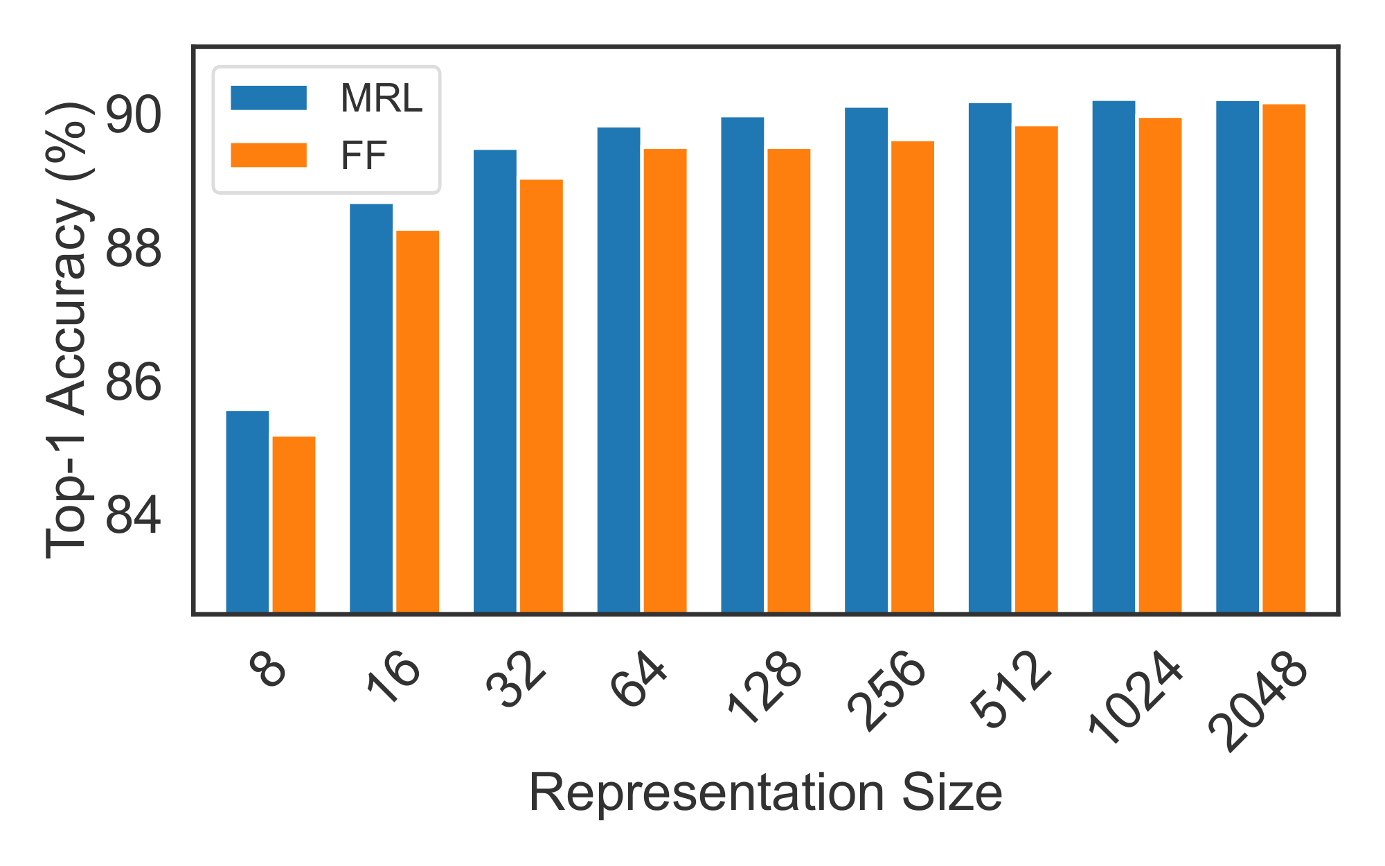
Figure 5 compares the linear classification accuracy of ResNet50 models trained and evaluated on ImageNet-1K. ResNet50– ${\rm MRL}$ model is at least as accurate as each FF model at every representation size in $\mathcal{M}$ while MRL–E is within $1%$ starting from $16$-dim. Similarly, Figure 6 showcases the comparison of learned representation quality through 1-NN accuracy on ImageNet-1K (trainset with 1.3M samples as the database and validation set with 50K samples as the queries). ${\rm Matryoshka~Representations}$ are up to $2%$ more accurate than their fixed-feature counterparts for the lower-dimensions while being as accurate elsewhere. 1-NN accuracy is an excellent proxy, at no additional training cost, to gauge the utility of learned representations in the downstream tasks.

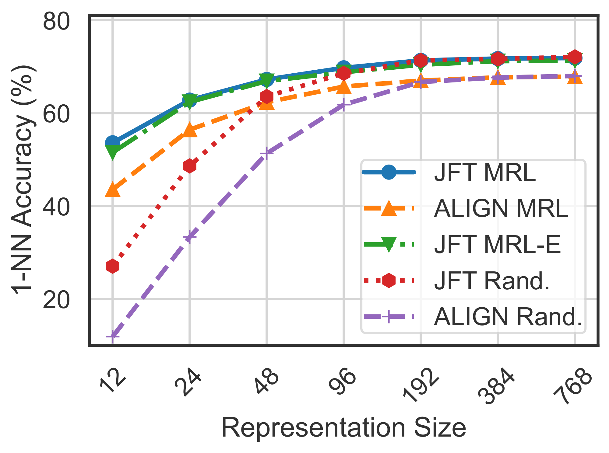
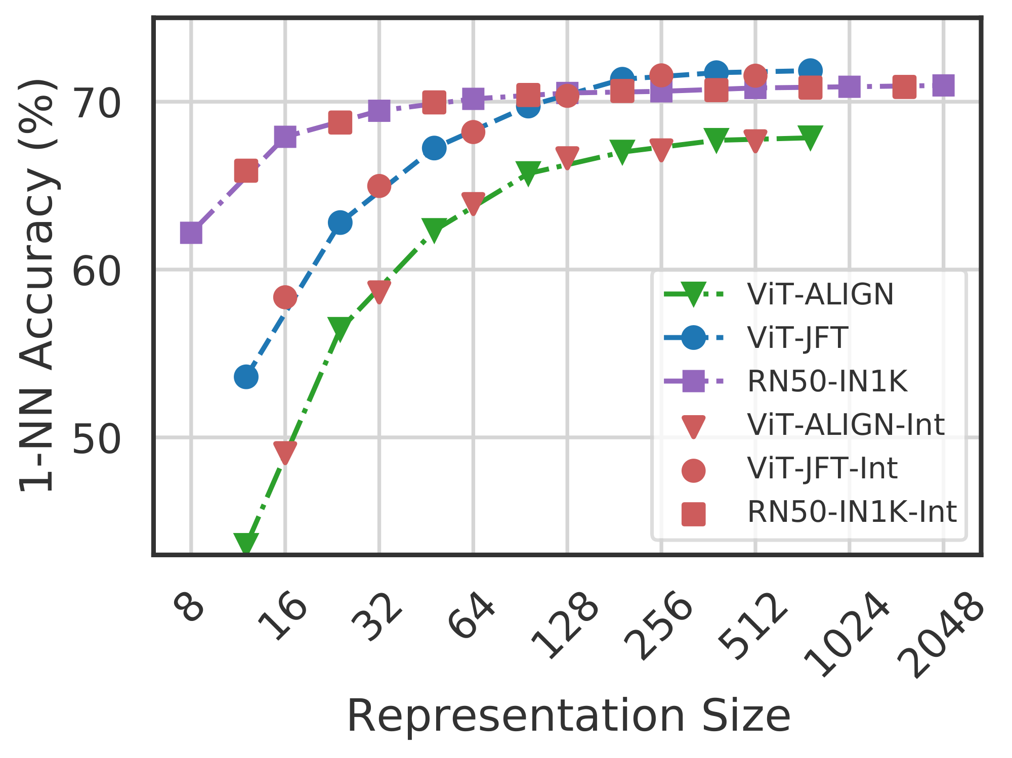
We also evaluate the quality of the representations from training ViT-B/16 on JFT-300M alongside the ViT-B/16 vision encoder of the ALIGN model – two web-scale setups. Due to the expensive nature of these experiments, we only train the highest capacity fixed feature model and choose random features for evaluation in lower-dimensions. Web-scale is a compelling setting for ${\rm MRL}$ due to its relatively inexpensive training overhead while providing multifidelity representations for downstream tasks. Figure 7, evaluated with 1-NN on ImageNet-1K, shows that all the ${\rm MRL}$ models for JFT and ALIGN are highly accurate while providing an excellent cost-vs-accuracy trade-off at lower-dimensions. These experiments show that ${\rm MRL}$ seamlessly scales to large-scale models and web-scale datasets while providing the otherwise prohibitively expensive multi-granularity in the process. We also have similar observations when pretraining BERT; please see Appendix D.2 for more details.

Our experiments also show that post-hoc compression (SVD), linear probe on random features, and sub-net style slimmable networks drastically lose accuracy compared to ${\rm MRL}$ as the representation size decreases. Finally, Figure 8 shows that, while ${\rm MRL}$ explicitly optimizes $O(\log(d))$ nested representations – removing the $O(d)$ dependence ([71]) –, the coarse-to-fine grained information is interpolated across all $d$ dimensions providing highest flexibility for adaptive deployment.

4.2.1 Adaptive Classification

The flexibility and coarse-to-fine granularity within ${\rm Matryoshka~Representations}$ allows model cascades ([74]) for Adaptive Classification (AC) ([10]). Unlike standard model cascades ([75]), ${\rm MRL}$ does not require multiple expensive neural network forward passes. To perform AC with an ${\rm MRL}$ trained model, we learn thresholds on the maximum softmax probability ([76]) for each nested classifier on a holdout validation set. We then use these thresholds to decide when to transition to the higher dimensional representation (e.g $8\to16\to32$) of the ${\rm MRL}$ model. Appendix D.1 discusses the implementation and learning of thresholds for cascades used for adaptive classification in detail.

Figure 9 shows the comparison between cascaded ${\rm MRL}$ representations (${\rm MRL}$ –AC) and independently trained fixed feature (FF) models on ImageNet-1K with ResNet50. We computed the expected representation size for ${\rm MRL}$ –AC based on the final dimensionality used in the cascade. We observed that ${\rm MRL}$ –AC was as accurate, $76.30%$, as a 512-dimensional FF model but required an expected dimensionality of $\sim37$ while being only $0.8%$ lower than the 2048-dimensional FF baseline. Note that all ${\rm MRL}$ –AC models are significantly more accurate than the FF baselines at comparable representation sizes. ${\rm MRL}$ –AC uses up to $\sim14\times$ smaller representation size for the same accuracy which affords computational efficiency as the label space grows ([7]). Lastly, our results with ${\rm MRL}$ –AC indicate that instances and classes vary in difficulty which we analyze in Section 5 and Appendix J.

4.3 Retrieval

Nearest neighbour search with learned representations powers a plethora of retrieval and search applications ([8, 3, 57, 2]). In this section, we discuss the image retrieval performance of the pretrained ResNet50 models (Section 4.1) on two large-scale datasets ImageNet-1K ([18]) and ImageNet-4K. ImageNet-1K has a database size of $\sim$ 1.3M and a query set of 50K samples uniformly spanning 1000 classes. We also introduce ImageNet-4K which has a database size of $\sim$ 4.2M and query set of $\sim$ 200K samples uniformly spanning 4202 classes (see Appendix B for details). A single forward pass on ResNet50 costs 4 GFLOPs while exact retrieval costs 2.6 GFLOPs per query for ImageNet-1K. Although retrieval overhead is $40%$ of the total cost, retrieval cost grows linearly with the size of the database. ImageNet-4K presents a retrieval benchmark where the exact search cost becomes the computational bottleneck ($8.6$ GFLOPs per query). In both these settings, the memory and disk usage are also often bottlenecked by the large databases. However, in most real-world applications exact search, $O(dN)$, is replaced with an approximate nearest neighbor search (ANNS) method like HNSW ([48]), $O(d\log(N))$, with minimal accuracy drop at the cost of additional memory overhead.

The goal of image retrieval is to find images that belong to the same class as the query using representations obtained from a pretrained model. In this section, we compare retrieval performance using mean Average Precision @ 10 (mAP@ $10$) which comprehensively captures the setup of relevant image retrieval at scale. We measure the cost per query using exact search in MFLOPs. All embeddings are unit normalized and retrieved using the L2 distance metric. Lastly, we report an extensive set of metrics spanning mAP@ $k$ and P@ $k$ for $k={10, 25, 50, 100}$ and real-world wall-clock times for exact search and HNSW. See Appendix E and Appendix F for more details.

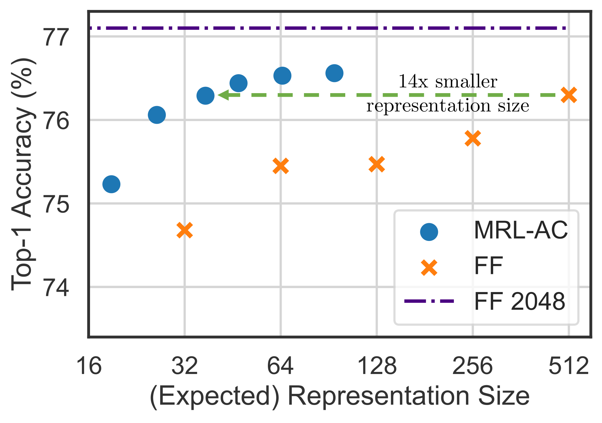
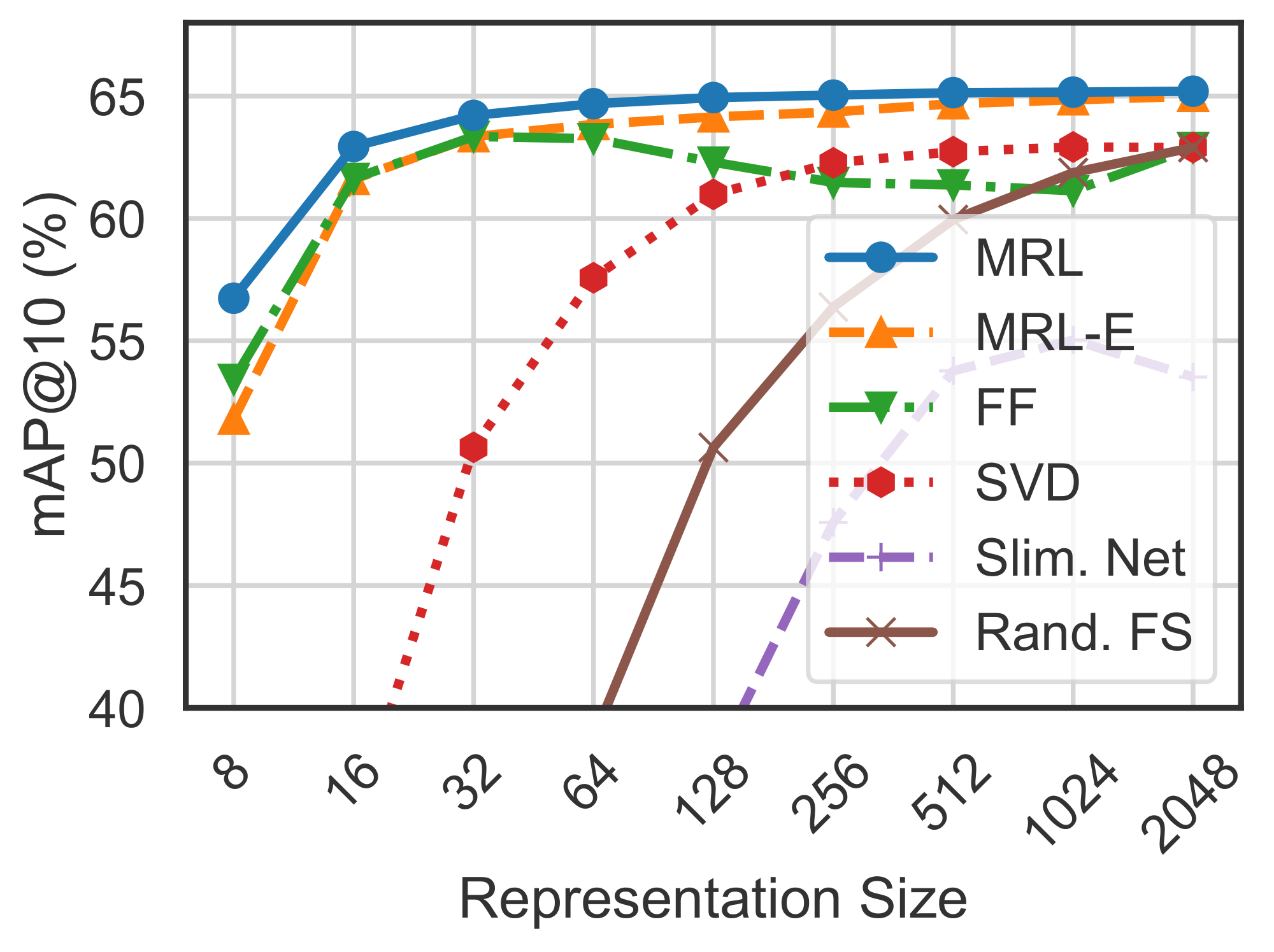
Figure 10 compares the mAP@ $10$ performance of ResNet50 representations on ImageNet-1K across dimensionalities for ${\rm MRL}$, MRL–E, FF, slimmable networks along with post-hoc compression of vectors using SVD and random feature selection. ${\rm Matryoshka~Representations}$ are often the most accurate while being up to $3%$ better than the FF baselines. Similar to classification, post-hoc compression and slimmable network baselines suffer from significant drop-off in retrieval mAP@ $10$ with $\le256$ dimensions. Appendix E discusses the mAP@ $10$ of the same models on ImageNet-4K.

${\rm MRL}$ models are capable of performing accurate retrieval at various granularities without the additional expense of multiple model forward passes for the web-scale databases. FF models also generate independent databases which become prohibitively expense to store and switch in between. ${\rm MatryoshkaRepresentations}$ enable adaptive retrieval (AR) which alleviates the need to use full-capacity representations, $d=2048$, for all data and downstream tasks. Lastly, all the vector compression techniques ([16, 77]) used as part of the ANNS pipelines are complimentary to ${\rm MatryoshkaRepresentations}$ and can further improve the efficiency-vs-accuracy trade-off.

4.3.1 Adaptive Retrieval

We benchmark ${\rm MRL}$ in the adaptive retrieval setting (AR) [6]. For a given query image, we obtained a shortlist, $K=200$, of images from the database using a lower-dimensional representation, e.g. $D_s=16$ followed by reranking with a higher capacity representation, e.g. $D_r=2048$. In real-world scenarios where top ranking performance is the key objective, measured with mAP@ $k$ where k covers a limited yet crucial real-estate, AR provides significant compute and memory gains over single-shot retrieval with representations of fixed dimensionality. Finally, the most expensive part of AR, as with any retrieval pipeline, is the nearest neighbour search for shortlisting. For example, even naive re-ranking of 200 images with 2048 dimensions only costs 400 KFLOPs. While we report exact search cost per query for all AR experiments, the shortlisting component of the pipeline can be sped-up using ANNS (HNSW). Appendix I has a detailed discussion on compute cost for exact search, memory overhead of HNSW indices and wall-clock times for both implementations. We note that using HNSW with 32 neighbours for shortlisting does not decrease accuracy during retrieval.

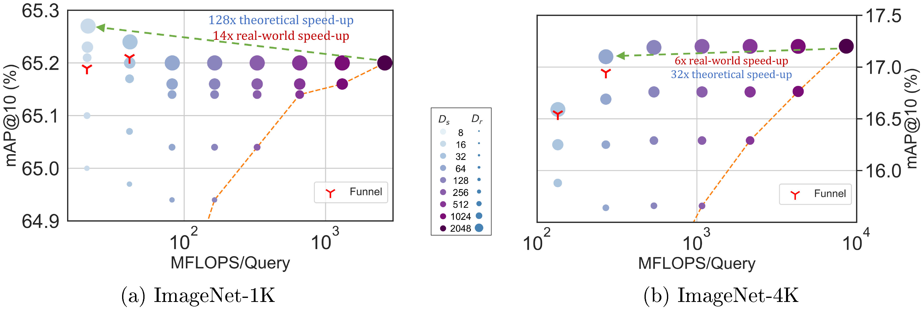
Figure 11 showcases the compute-vs-accuracy trade-off for adaptive retrieval using ${\rm MatryoshkaRepresentations}$ compared to single-shot using fixed features with ResNet50 on ImageNet-1K. We observed that all AR settings lied above the Pareto frontier of single-shot retrieval with varying representation sizes. In particular for ImageNet-1K, we show that the AR model with $D_s=16$ & $D_r=2048$ is as accurate as single-shot retrieval with $d=2048$ while being $\mathbf{\sim128\times}$ more efficient in theory and $\mathbf{\sim14\times}$ faster in practice (compared using HNSW on the same hardware). We show similar trends with ImageNet-4K, but note that we require $D_s=64$ given the increased difficulty of the dataset. This results in $\sim32\times$ and $\sim6\times$ theoretical and in-practice speedups respectively. Lastly, while $K=200$ works well for our adaptive retrieval experiments, we ablated over the shortlist size $k$ in Appendix K.2 and found that the accuracy gains stopped after a point, further strengthening the use-case for ${\rm MatryoshkaRepresentation~Learning}$ and adaptive retrieval.

Even with adaptive retrieval, it is hard to determine the choice of $D_s$ & $D_r$. In order to alleviate this issue to an extent, we propose Funnel Retrieval, a consistent cascade for adaptive retrieval. Funnel thins out the initial shortlist by a repeated re-ranking and shortlisting with a series of increasing capacity representations. Funnel halves the shortlist size and doubles the representation size at every step of re-ranking. For example on ImageNet-1K, a funnel with the shortlist progression of $200\to100\to50\to25\to10$ with the cascade of $16\to32\to64\to128\to256\to2048$ representation sizes within ${\rm Matryoshka~Representation}$ is as accurate as the single-shot 2048-dim retrieval while being $\sim128\times$ more efficient theoretically (see Appendix F for more results). All these results showcase the potential of ${\rm MRL}$ and AR for large-scale multi-stage search systems ([8]).

5. Further Analysis and Ablations

Section Summary: The section explores the robustness of Matryoshka Representations (MRL) models, showing they handle out-of-domain images and retrieval tasks as well as or better than standard models, with notable improvements in accuracy on challenging datasets and zero-shot scenarios. In few-shot and long-tail learning, MRL performs comparably or superior, especially for rare classes, while lower-dimensional representations sometimes excel due to less confusion from irrelevant details, revealing how these models naturally capture broader category hierarchies. Ablations demonstrate that MRL can be efficiently added to existing pretrained models through minimal fine-tuning, highlighting their potential for widespread use in analyzing and adapting information efficiency.

Robustness.

We evaluate the robustness of the ${\rm MRL}$ models trained on ImageNet-1K on out-of-domain datasets, ImageNetV2/R/A/Sketch ([78, 79, 80, 81]), and compare them to the FF baselines. Table 17 in Appendix H demonstrates that ${\rm Matryoshka~Representations}$ for classification are at least as robust as the original representation while improving the performance on ImageNet-A by $0.6%$ – a $20%$ relative improvement. We also study the robustness in the context of retrieval by using ImageNetV2 as the query set for ImageNet-1K database. Table 9 in Appendix E shows that ${\rm MRL}$ models have more robust retrieval compared to the FF baselines by having up to $3%$ higher mAP@ $10$ performance. This observation also suggests the need for further investigation into robustness using nearest neighbour based classification and retrieval instead of the standard linear probing setup. We also find that the zero-shot robustness of ALIGN- ${\rm MRL}$ (Table 18 in Appendix H) agrees with the observations made by [82]. Lastly, Table 6 in Appendix D.2 shows that ${\rm MRL}$ also improves the cosine similarity span between positive and random image-text pairs.

Few-shot and Long-tail Learning.

We exhaustively evaluated few-shot learning on ${\rm MRL}$ models using nearest class mean ([83]). Table 15 in Appendix G shows that that representations learned through ${\rm MRL}$ perform comparably to FF representations across varying shots and number of classes.

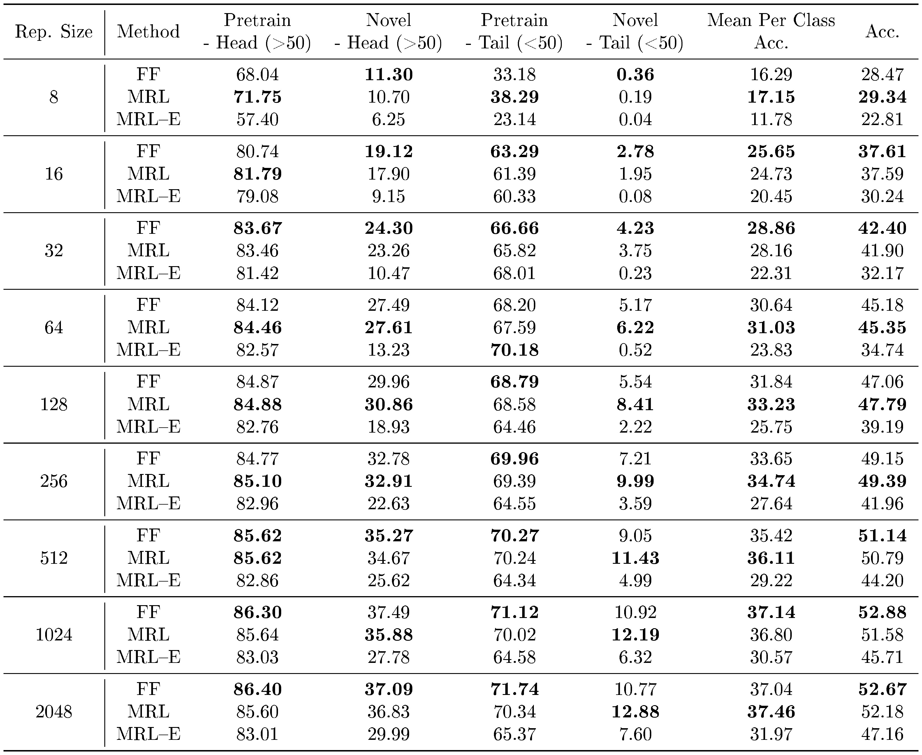
${\rm Matryoshka~Representations}$ realize a unique pattern while evaluating on FLUID ([84]), a long-tail sequential learning framework. We observed that ${\rm MRL}$ provides up to $2%$ accuracy higher on novel classes in the tail of the distribution, without sacrificing accuracy on other classes (Table 16 in Appendix G). Additionally we find the accuracy between low-dimensional and high-dimensional representations is marginal for pretrain classes. We hypothesize that the higher-dimensional representations are required to differentiate the classes when few training examples of each are known. This results provides further evidence that different tasks require varying capacity based on their difficulty.

Disagreement across Dimensions.

The information packing in ${\rm Matryoshka~Representations}$ often results in gradual increase of accuracy with increase in capacity. However, we observed that this trend was not ubiquitous and certain instances and classes were more accurate when evaluated with lower-dimensions (Figure 15 in Appendix J). With perfect routing of instances to appropriate dimension, ${\rm MRL}$ can gain up to $4.6%$ classification accuracy. At the same time, the low-dimensional models are less accurate either due to confusion within the same superclass ([86]) of the ImageNet hierarchy or presence of multiple objects of interest. Figure 12 showcases 2 such examples for $8$-dimensional representation. These results along with Appendix J put forward the potential for ${\rm MRL}$ to be a systematic framework for analyzing the utility and efficiency of information bottlenecks.

Superclass Accuracy.

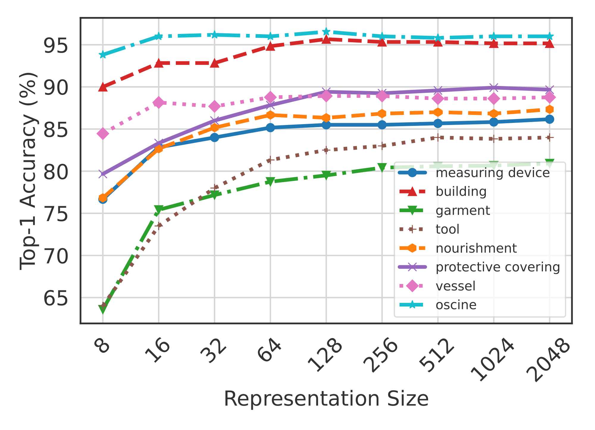
As the information bottleneck becomes smaller, the overall accuracy on fine-grained classes decreases rapidly (Figure 6). However, the drop-off is not as significant when evaluated at a superclass level (Table 24 in Appendix J). Figure 13 presents that this phenomenon occurs with both ${\rm MRL}$ and FF models; ${\rm MRL}$ is more accurate across dimensions. This shows that tight information bottlenecks while not highly accurate for fine-grained classification, do capture required semantic information for coarser classification that could be leveraged for adaptive routing for retrieval and classification. Mutifidelity of ${\rm Matryoshka~Representation}$ naturally captures the underlying hierarchy of the class labels with one single model. Lastly, Figure 14 showcases the accuracy trends per superclass with ${\rm MRL}$. The utility of additional dimensions in distinguishing a class from others within the same superclass is evident for "garment" which has up to 11% improvement for 8 $\to$ 16 dimensional representation transition. We also observed that superclasses such as "oscine (songbird)" had a clear visual distinction between the object and background and thus predictions using 8 dimensions also led to a good inter-class separability within the superclass.

5.1 Ablations

Table 26 in Appendix K presents that ${\rm Matryoshka~Representations}$ can be enabled within off-the-shelf pretrained models with inexpensive partial finetuning thus paving a way for ubiquitous adoption of ${\rm MRL}$. At the same time, Table 27 in Appendix C indicates that with optimal weighting of the nested losses we could improve accuracy of lower-dimensions representations without accuracy loss. Table 28 and Table 29 in Appendix C ablate over the choice of initial granularity and spacing of the granularites. Table 28 reaffirms the design choice to shun extremely low dimensions that have poor classification accuracy as initial granularity for ${\rm MRL}$ while Table 29 confirms the effectiveness of logarthmic granularity spacing inspired from the behaviour of accuracy saturation across dimensions over uniform. Lastly, Table 30 and Table 31 in Appendix K.2 show that the retrieval performance saturates after a certain shortlist dimension and length depending on the complexity of the dataset.

6. Discussion and Conclusions

Section Summary: The section discusses potential improvements for Matryoshka Representation Learning (MRL), a method that packs information at different levels into a single vector to adapt to varying task demands and computing power, suggesting future work like better balancing of training goals, tailored loss functions, and smarter data structures for faster searches. In wrapping up, it highlights MRL's applications in adaptive classification and retrieval, where it achieves similar accuracy to standard approaches but with much smaller data sizes—about 14 times tinier on average—and dramatic efficiency gains, like 128 times fewer computations and 14 times quicker runtimes. These benefits pair well with other speed-up techniques, making MRL ideal for resource-limited settings.

The results in Section 5.1 reveal interesting weaknesses of ${\rm MRL}$ that would be logical directions for future work. (1) Optimizing the weightings of the nested losses to obtain a Pareto optimal accuracy-vs-efficiency trade-off – a potential solution could emerge from adaptive loss balancing aspects of anytime neural networks ([87]). (2) Using different losses at various fidelities aimed at solving a specific aspect of adaptive deployment – e.g. high recall for $8$-dimension and robustness for $2048$-dimension. (3) Learning a search data-structure, like differentiable k-d tree, on top of ${\rm Matryoshka~Representation}$ to enable dataset and representation aware retrieval. (4) Finally, the joint optimization of multi-objective ${\rm MRL}$ combined with end-to-end learnable search data-structure to have data-driven adaptive large-scale retrieval for web-scale search applications.

In conclusion, we presented ${\rm MatryoshkaRepresentationLearning}$ (${\rm MRL}$), a flexible representation learning approach that encodes information at multiple granularities in a single embedding vector. This enables the ${\rm MRL}$ to adapt to a downstream task's statistical complexity as well as the available compute resources. We demonstrate that ${\rm MRL}$ can be used for large-scale adaptive classification as well as adaptive retrieval. On standard benchmarks, ${\rm MRL}$ matches the accuracy of the fixed-feature baseline despite using $14\times$ smaller representation size on average. Furthermore, the ${\rm Matryoshka~Representation}$ based adaptive shortlisting and re-ranking system ensures comparable mAP@ $10$ to the baseline while being $128\times$ cheaper in FLOPs and $14\times$ faster in wall-clock time. Finally, most of the efficiency techniques for model inference and vector search are complementary to ${\rm MRL}$ further assisting in deployment at the compute-extreme environments.

Acknowledgments

Section Summary: The acknowledgments express gratitude to several researchers, including Srinadh Bhojanapalli, Lovish Madaan, Raghav Somani, Ludwig Schmidt, and Venkata Sailesh Sanampudi, for their helpful discussions and feedback on the work. Aditya Kusupati specifically thanks Tom Duerig and Rahul Sukthankar for their support, while large-scale experiments were enabled by research credits from Google Cloud and Google Research. Additional funding came from various sources, such as the CONIX Research Center for Gantavya Bhatt, NSF and ONR grants for Sham Kakade, and NSF, DARPA awards plus gifts from the Allen Institute for Ali Farhadi.

We are grateful to Srinadh Bhojanapalli, Lovish Madaan, Raghav Somani, Ludwig Schmidt, and Venkata Sailesh Sanampudi for helpful discussions and feedback. Aditya Kusupati also thanks Tom Duerig and Rahul Sukthankar for their support. Part of the paper's large-scale experimentation is supported through a research GCP credit award from Google Cloud and Google Research. Gantavya Bhatt is supported in part by the CONIX Research Center, one of six centers in JUMP, a Semiconductor Research Corporation (SRC) program sponsored by DARPA. Sham Kakade acknowledges funding from the NSF award CCF-1703574 and ONR N00014-22-1-2377. Ali Farhadi acknowledges funding from the NSF awards IIS 1652052, IIS 17303166, DARPA N66001-19-2-4031, DARPA W911NF-15-1-0543 and gifts from Allen Institute for Artificial Intelligence.

Checklist

Appendix

Section Summary: The appendix provides Python code templates for implementing Matryoshka Representation Learning (MRL), a technique that trains models like ResNet50 to produce flexible image representations of varying sizes, using custom loss functions and linear layers for datasets such as ImageNet. It details several image datasets, including the standard ImageNet-1K with over a million labeled photos across 1,000 categories, larger ones like JFT-300M and ALIGN for robust training, and specialized sets like ImageNet-A for testing real-world challenges. Training procedures cover efficient setups with tools like FFCV on GPUs or TPUs, hyperparameters for different model variants, and an overview of classification accuracy results in tables.

A. Code for ${\rm MatryoshkaRepresentationLearning}$ (${\rm MRL}$)

We use Algorithm 1 and Algorithm 2 provided below to train supervised ResNet50– ${\rm MRL}$ models on ImageNet-1K. We provide this code as a template to extend ${\rm MRL}$ to any domain.

class Matryoshka_CE_Loss(nn.Module):
    def __init__(self, relative_importance, **kwargs):
        super(Matryoshka_CE_Loss, self).__init__()
        self.criterion = nn.CrossEntropyLoss(**kwargs)
        self.relative_importance = relative_importance # usually set to all ones

  def forward(self, output, target):
        loss=0
        for i in range(len(output)):
          loss+= self.relative_importance[i] * self.criterion(output[i], target)
        return loss

class MRL_Linear_Layer(nn.Module):
    def __init__(self, nesting_list: List, num_classes=1000, efficient=False, **kwargs):
        super(MRL_Linear_Layer, self).__init__()
        self.nesting_list=nesting_list # set of m in M (Eq. 1)
        self.num_classes=num_classes 
        self.is_efficient=efficient # flag for MRL-E

            if not is_efficient:
                for i, num_feat in enumerate(self.nesting_list):
                    setattr(self, f"nesting_classifier_{i}", nn.Linear(num_feat, self.num_classes, **kwargs))
            else:
                setattr(self, "nesting_classifier_0", nn.Linear(self.nesting_list[-1], self.num_classes, **kwargs)) # Instantiating one nn.Linear layer for MRL-E

        def forward(self, x):
            nesting_logits = ()
            for i, num_feat in enumerate(self.nesting_list):
                if(self.is_efficient):
                    efficient_logit = torch.matmul(x[:, :num_feat], (self.nesting_classifier_0.weight[:, :num_feat]).t())
                else:
                    nesting_logits.append(getattr(self, f"nesting_classifier_{i}")(x[:, :num_feat]))

            if(self.is_efficient):
                nesting_logits.append(efficient_logit)

            return nesting_logits

B. Datasets

ImageNet-1K ([18]) contains 1, 281, 167 labeled train images, and 50, 000 labelled validation images across 1, 000 classes. The images were transformed with standard procedures detailed by FFCV ([90]).

ImageNet-4K dataset was constructed by selecting 4, 202 classes, non-overlapping with ImageNet-1K, from ImageNet-21K ([17]) with 1, 050 or more examples. The train set contains 1, 000 examples and the query/validation set contains 50 examples per class totalling to $\sim$ 4.2M and $\sim$ 200K respectively. We will release the list of images curated together to construct ImageNet-4K.

JFT-300M ([9]) is a large-scale multi-label dataset with 300M images labelled across 18, 291 categories.

ALIGN ([30]) utilizes a large scale noisy image-text dataset containing 1.8B image-text pairs.

ImageNet Robustness Datasets

We experimented on the following datasets to examine the robustness of ${\rm MRL}$ models:

ImageNetV2 ([78]) is a collection of 10K images sampled a decade after the original construction of ImageNet ([17]). ImageNetV2 contains 10 examples each from the 1, 000 classes of ImageNet-1K.

ImageNet-A ([80]) contains 7.5K real-world adversarially filtered images from 200 ImageNet-1K classes.

ImageNet-R ([79]) contains 30K artistic image renditions for 200 of the original ImageNet-1K classes.

ImageNet-Sketch ([81]) contains 50K sketches, evenly distributed over all 1, 000 ImageNet-1K classes.

ObjectNet ([91]) contains 50K images across 313 object classes, each containing $\sim$ 160 images each.

C. ${\rm MatryoshkaRepresentationLearning}$ Model Training

We trained all ResNet50– ${\rm MRL}$ models using the efficient dataloaders of FFCV ([90]). We utilized the rn50_40_epochs.yaml configuration file of FFCV to train all ${\rm MRL}$ models defined below:

• ${\rm MRL}$: ResNet50 model with the fc layer replaced by MRL_Linear_Layer(efficient=False)
• MRL–E: ResNet50 model with the fc layer replaced by MRL_Linear_Layer(efficient=True)
• FF–k: ResNet50 model with the fc layer replaced by torch.nn.Linear(k, num_classes), where k $\in [8, 16, 32, 64, 128, 256, 512, 1024, 2048]$. We will henceforth refer to these models as simply FF, with the k value denoting representation size.

We trained all ResNet50 models with a learning rate of $0.475$ with a cyclic learning rate schedule ([92]). This was after appropriate scaling (0.25 $\times$) of the learning rate specified in the configuration file to accommodate for 2xA100 NVIDIA GPUs available for training, compared to the 8xA100 GPUs utilized in the FFCV benchmarks. We trained with a batch size of 256 per GPU, momentum ([93]) of 0.9, and an SGD optimizer with a weight decay of 1e-4.

Our code (Appendix A) makes minimal modifications to the training pipeline provided by FFCV to learn ${\rm Matryoshka~Representations}$.

We trained ViT-B/16 models for JFT-300M on a 8x8 cloud TPU pod ([94]) using Tensorflow ([95]) with a batchsize of 128 and trained for 300K steps. Similarly, ALIGN models were trained using Tensorflow on 8x8 cloud TPU pod for 1M steps with a batchsize of 64 per TPU. Both these models were trained with adafactor optimizer ([96]) with a linear learning rate decay starting at 1e-3.

Lastly, we trained a BERT-Base model on English Wikipedia and BookCorpus. We trained our models in Tensorflow using a 4x4 cloud TPU pod with a total batchsize of 1024. We used AdamW ([97]) optimizer with a linear learning rate decay starting at 1e-4 and trained for 450K steps.

In each configuration/case, if the final representation was normalized in the FF implementation, ${\rm MRL}$ models adopted the same for each nested dimension for a fair comparison.

D. Classification Results

: Table 1: Top-1 classification accuracy (%) for ResNet50 $MRL$ and baseline models on ImageNet-1K.

Rep. Size	Rand. LP	SVD	FF	Slim. Net	${\rm MRL}$	MRL–E
8	4.56	2.34	65.29	0.42	66.63	56.66
16	11.29	7.17	72.85	0.96	73.53	71.94
32	27.21	20.46	74.60	2.27	75.03	74.48
64	49.47	48.10	75.27	5.59	75.82	75.35
128	65.70	67.24	75.29	14.15	76.30	75.80
256	72.43	74.59	75.71	38.42	76.47	76.22
512	74.94	76.78	76.18	69.80	76.65	76.36
1024	76.10	76.87	76.63	74.61	76.76	76.48
2048	76.87	–	76.87	76.26	76.80	76.51

We show the top-1 classification accuracy of ResNet50– ${\rm MRL}$ models on ImageNet-1K in Table 1 and Figure 5. We compare the performance of ${\rm MRL}$ models (${\rm MRL}$, MRL–E) to several baselines:

• FF: We utilize the FF-k models described in Appendix C for $k\in{8, ... 2048}$.
• SVD: We performed a low rank approximation of the 1000-way classification layer of FF-2048, with rank = 1000.
• Rand. LP: We compared against a linear classifier fit on randomly selected features ([26]).
• Slim. Net: We take pretrained slimmable neural networks ([14]) which are trained with a flexible width backbone (25%, 50%, 75% and full width). For each representation size, we consider the first $k$ dimensions for classification. Note that training of slimmable neural networks becomes unstable when trained below 25% width due to the hardness in optimization and low complexity of the model.

At lower dimensions ($d \leq 128$), ${\rm MRL}$ outperforms all baselines significantly, which indicates that pretrained models lack the multifidelity of ${\rm Matryoshka~Representations}$ and are incapable of fitting an accurate linear classifier at low representation sizes.

We compared the performance of ${\rm MRL}$ models at various representation sizes via 1-nearest neighbors (1-NN) image classification accuracy on ImageNet-1K in Figure 6 and Figure 6. We provide detailed information regarding the k-NN search pipeline in Appendix E. We compared against a baseline of attempting to enforce nesting to a FF-2048 model by 1) Random Feature Selection (Rand. FS): considering the first $m$ dimensions of FF-2048 for NN lookup, and 2) FF+SVD: performing SVD on the FF-2048 representations at the specified representation size, 3) FF+JL: performing random projection according to the Johnson-Lindenstrauss lemma ([98]) on the FF-2048 representations at the specified representation size. We also compared against the 1-NN accuracy of slimmable neural nets ([14]) as an additional baseline. We observed these baseline models to perform very poorly at lower dimensions, as they were not explicitly trained to learn ${\rm Matryoshka~Representations}$.

: Table 2: 1-NN accuracy (%) on ImageNet-1K for various ResNet50 models.

Rep. Size	Rand. FS	SVD	JL	FF	Slimmable	${\rm MRL}$	MRL–E
8	2.36	19.14	0.11	58.93	1.00	62.19	57.45
16	12.06	46.02	0.09	66.77	5.12	67.91	67.05
32	32.91	60.78	0.06	68.84	16.95	69.46	68.6
64	49.91	67.04	0.05	69.41	35.60	70.17	69.61
128	60.91	69.63	0.06	69.35	51.16	70.52	70.12
256	65.75	70.67	0.04	69.72	60.61	70.62	70.36
512	68.77	71.06	0.03	70.18	65.82	70.82	70.74
1024	70.41	71.22	-	70.34	67.19	70.89	71.07
2048	71.19	71.21	-	71.19	66.10	70.97	71.21

D.1 Adaptive Classification (${\rm MRL}$ –AC)

: Table 3: Threshold-based adaptive classification performance of ResNet50 $MRL$ on a 40K sized held-out subset of the ImageNet-1K validation set. Results are averaged over 30 random held-out subsets.

Expected Rep. Size	Accuracy
13.43 $\pm$ 0.81	73.79 $\pm$ 0.10
18.32 $\pm$ 1.36	75.25 $\pm$ 0.11
25.87 $\pm$ 2.41	76.05 $\pm$ 0.15
36.26 $\pm$ 4.78	76.28 $\pm$ 0.16
48.00 $\pm$ 8.24	76.43 $\pm$ 0.18
64.39 $\pm$ 12.55	76.53 $\pm$ 0.19
90.22 $\pm$ 20.88	76.55 $\pm$ 0.20
118.85 $\pm$ 33.37	76.56 $\pm$ 0.20

In an attempt to use the smallest representation that works well for classification for every image in the ImageNet-1K validation set, we learned a policy to increase the representation size from $m_i$ to $m_{i+1}$ using a 10K sized subset of the ImageNet-1K validation set. This policy is based on whether the prediction confidence $p_i$ using representation size $m_i$ exceeds a learned threshold $t_{i}^{\ast}$. If $p_i \geq t_{i}^{\ast}$, we used predictions from representation size $m_i$ otherwise, we increased to representation size $m_{i+1}$. To learn the optimal threshold $t_{i}^{\ast}$, we performed a grid search between 0 and 1 (100 samples). For each threshold $t_k$, we computed the classification accuracy over our 10K image subset. We set $t_{i}^{\ast}$ equal to the smallest threshold $t_k$ that gave the best accuracy. We use this procedure to obtain thresholds for successive models, i.e., ${t_{j}^{\ast} \mid j \in {8, 16, 32, 64, \ldots, 2048}}$. To improve reliability of threshold based greedy policy, we use test time augmentation which has been used successfully in the past ([21]).

For inference, we used the remaining held-out 40K samples from the ImageNet-1K validation set. We began with smallest sized representation ($m = 8$) and compared the computed prediction confidence $p_8$ to learned optimal threshold $t_8^{\ast}$. If $p_8 \leq t_8^{\ast}$, then we increased $m = 16$, and repeated this procedure until $m = d = 2048$. To compute the expected dimensions, we performed early stopping at $m = {16, 32, 64, \ldots 2048}$ and computed the expectation using the distribution of representation sizes. As shown in Table 3 and Figure 9, we observed that in expectation, we only needed a $\sim37$ sized representation to achieve $76.3%$ classification accuracy on ImageNet-1K, which was roughly $14\times$ smaller than the FF–512 baseline. Even if we computed the expectation as a weighted average over the cumulative sum of representation sizes ${8, 24, 56, \ldots}$, due to the nature of multiple linear heads for ${\rm MRL}$, we ended up with an expected size of $62$ that still provided a roughly $8.2\times$ efficient representation than the FF–512 baseline. However, MRL–E alleviates this extra compute with a minimal drop in accuracy.

D.2 JFT, ALIGN and BERT

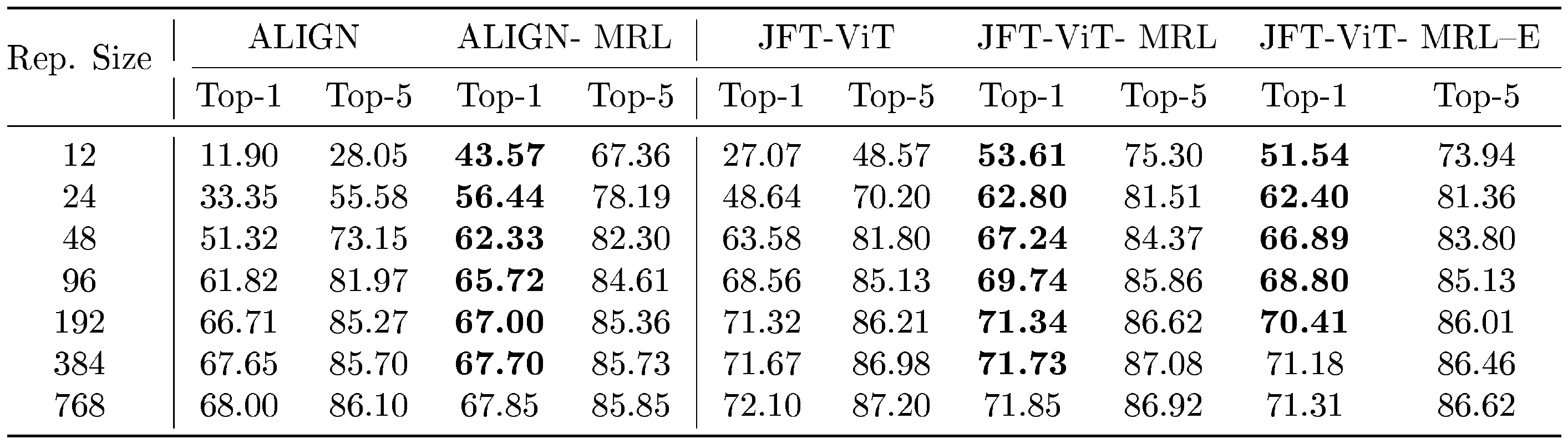
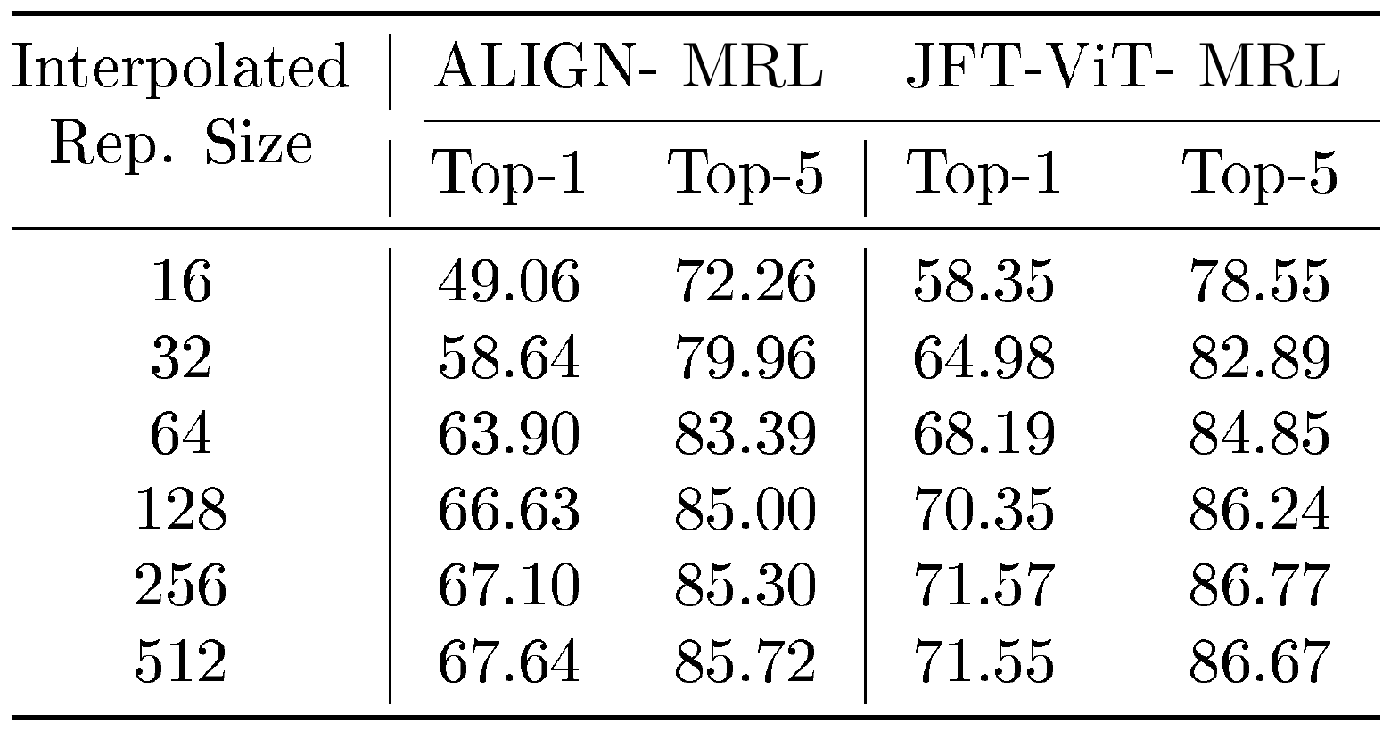
We examine the k-NN classification accuracy of learned ${\rm MatryoshkaRepresentations}$ via ALIGN– ${\rm MRL}$ and JFT-ViT– ${\rm MRL}$ in Table 4. For ALIGN ([30]), we observed that learning ${\rm MatryoshkaRepresentations}$ via ALIGN– ${\rm MRL}$ improved classification accuracy at nearly all dimensions when compared to ALIGN. We observed a similar trend when training ViT-B/16 ([72]) for JFT-300M ([9]) classification, where learning ${\rm MatryoshkaRepresentations}$ via ${\rm MRL}$ and MRL–E on top of JFT-ViT improved classification accuracy for nearly all dimensions, and significantly for lower ones. This demonstrates that training to learn ${\rm MatryoshkaRepresentations}$ is feasible and extendable even for extremely large scale datasets. We also demonstrate that ${\rm Matryoshka~Representations}$ are learned at interpolated dimensions for both ALIGN and JFT-ViT, as shown in Table 5, despite not being trained explicitly at these dimensions. Lastly, Table 6 shows that ${\rm MRL}$ training leads to a increase in the cosine similarity span between positive and random image-text pairs.

::: {caption="Table 4: ViT-B/16 and ViT-B/16- $MRL$ top-1 and top-5 k-NN accuracy (%) for ALIGN and JFT. Top-1 entries where MRL–E and $MRL$ outperform baselines are bolded for both ALIGN and JFT-ViT."}

:::

::: {caption="Table 5: Examining top-1 and top-5 k-NN accuracy (%) at interpolated hidden dimensions for ALIGN and JFT. This indicates that $MRL$ is able to scale classification accuracy as hidden dimensions increase even at dimensions that were not explicitly considered during training."}

:::

: Table 6: Cosine similarity between embeddings

Avg. Cosine Similarity	ALIGN	ALIGN- ${\rm MRL}$
Positive Text to Image	0.27	0.49
Random Text to Image	8e-3	-4e-03
Random Image to Image	0.10	0.08
Random Text to Text	0.22	0.07

We also evaluated the capability of ${\rm MatryoshkaRepresentations}$ to extend to other natural language processing via masked language modeling (MLM) with BERT ([37]), whose results are tabulated in Table 7. Without any hyper-parameter tuning, we observed ${\rm MatryoshkaRepresentations}$ to be within $0.5%$ of FF representations for BERT MLM validation accuracy. This is a promising initial result that could help with large-scale adaptive document retrieval using BERT– ${\rm MRL}$.

: Table 7: Masked Language Modelling (MLM) accuracy(%) of FF and $MRL$ models on the validation set.

Rep. Size	BERT- FF	BERT- ${\rm MRL}$
12	60.12	59.92
24	62.49	62.05
48	63.85	63.40
96	64.32	64.15
192	64.70	64.58
384	65.03	64.81
768	65.54	65.00

E. Image Retrieval

We evaluated the strength of ${\rm Matryoshka~Representations}$ via image retrieval on ImageNet-1K (the training distribution), as well as on out-of-domain datasets ImageNetV2 and ImageNet-4K for all ${\rm MRL}$ ResNet50 models. We generated the database and query sets, containing $N$ and $Q$ samples respectively, with a standard PyTorch ([99]) forward pass on each dataset. We specify the representation size at which we retrieve a shortlist of k-nearest neighbors (k-NN) by $D_s$. The database is a thus a [$N$, $D_s$] array, the query set is a [$Q$, $D_s$] array, and the neighbors set is a [$Q$, k] array. For metrics, we utilized corrected mean average precision (mAP@k) ([50]) and precision (P@k): $P@k = \dfrac{correct_pred}{k}$ where $correct_pred$ is the average number of retrieved NN with the correct label over the entire query set using a shortlist of length $k$.

We performed retrieval with FAISS ([100]), a library for efficient similarity search. To obtain a shortlist of k-NN, we built an index to search the database. We performed an exhaustive NN search with the L2 distance metric with faiss.IndexFlatL2, as well as an approximate NN search (ANNS) via HNSW ([100]) with faiss.IndexHNSWFlat. We used HNSW with $M = 32$ unless otherwise mentioned, and henceforth referred to as HNSW32. The exact search index was moved to the GPU for fast k-NN search computation, whereas the HNSW index was kept on the CPU as it currently lacks GPU support. We show the wall clock times for building the index as well as the index size in Table 20. We observed exact search to have a smaller index size which was faster to build when compared to HNSW, which trades off a larger index footprint for fast NN search (discussed in more detail in Appendix K). The database and query vectors are normalized with faiss.normalize_L2 before building the index and performing search.

::: {caption="Table 8: Retrieve a shortlist of 200-NN with $D_s$ sized representations on ImageNet-1K via exact search with L2 distance metric. Top-1 and mAP@10 entries (%) where MRL–E and $MRL$ outperform FF at their respective representation sizes are bolded."}

:::

::: {caption="Table 9: Retrieve a shortlist of 200-NN with $D_s$ sized representations on ImageNetV2 via exact search with L2 distance metric. Top-1 and mAP@10 entries (%) where MRL–E outperforms FF are bolded. $MRL$ outperforms FF at all $D_s$ and is thus not bolded."}

:::

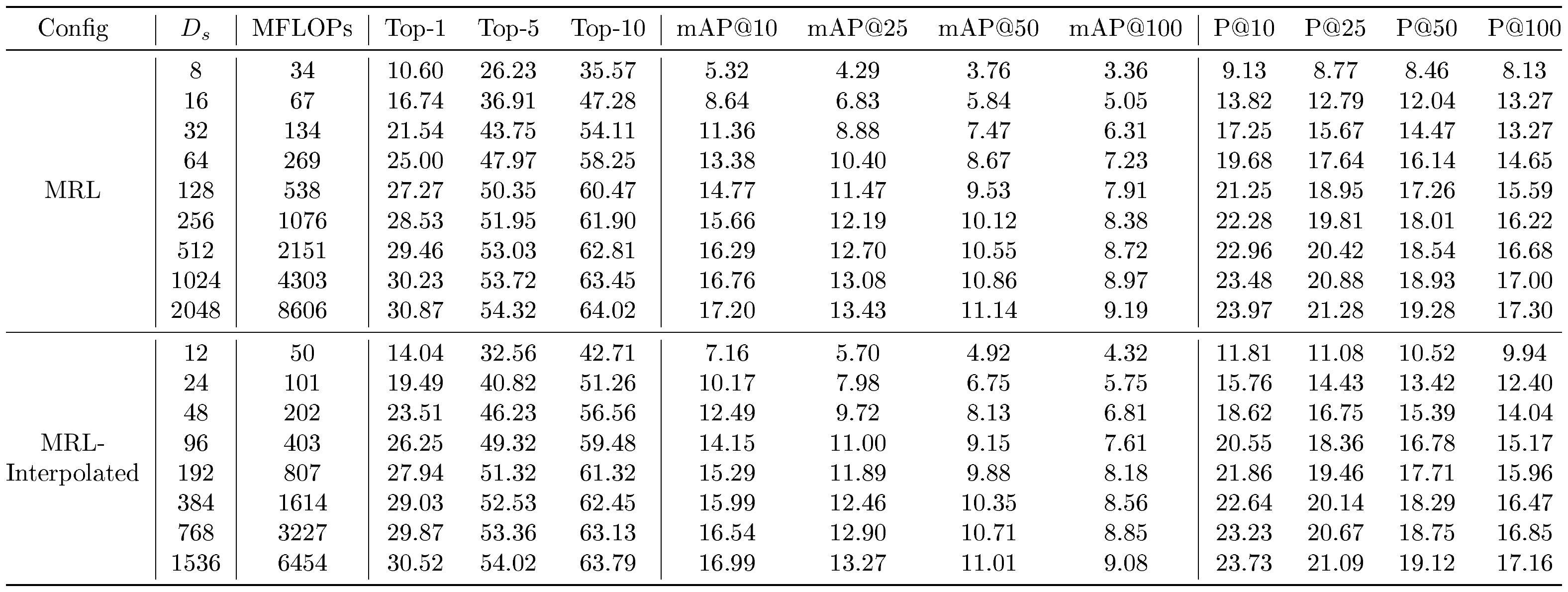
::: {caption="Table 10: Retrieve a shortlist of 200-NN with $D_s$ sized representations on ImageNet-4K via exact search with L2 distance metric. MRL–E and FF models are omitted for clarity and compute/inference time costs. All entries are in %."}

:::

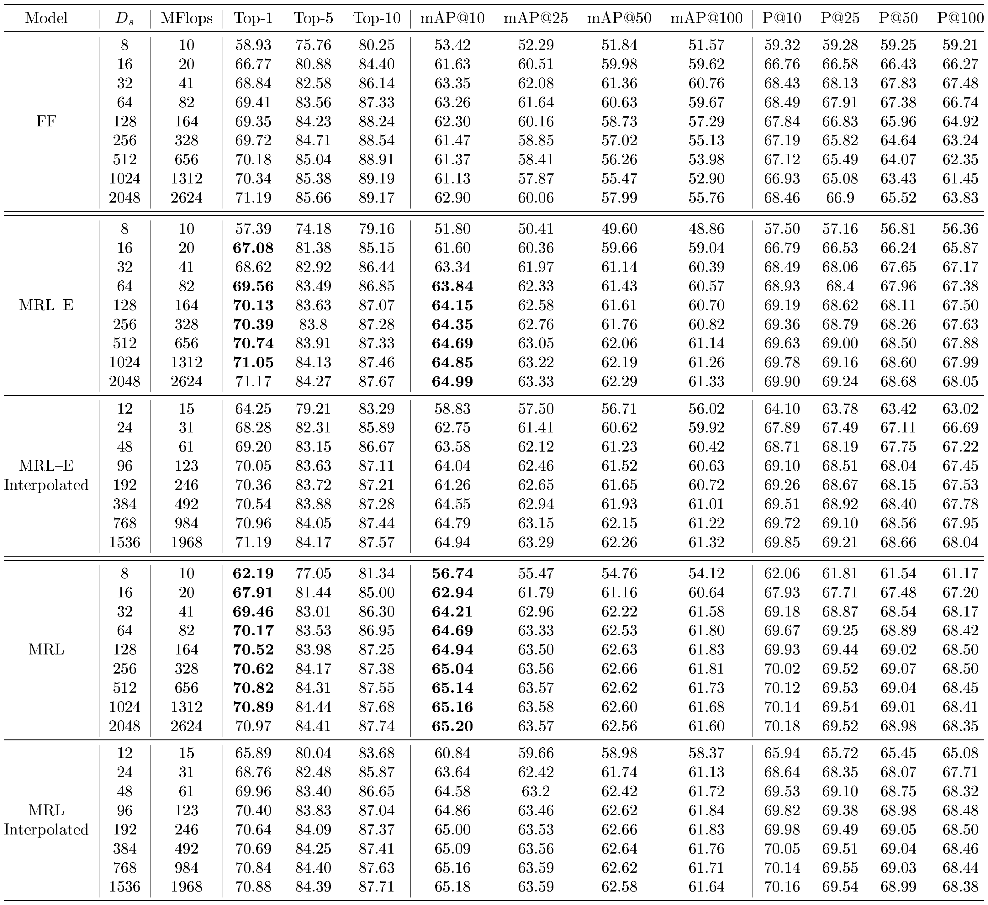
Retrieval performance on ImageNet-1K, i.e. the training distribution, is shown in Table 8. ${\rm MRL}$ outperforms FF models for nearly all representation size for both top-1 and mAP@10, and especially at low representation size ($D_s$ $\leq 32$). MRL–E loses out to FF significantly only at $D_s$ $ = 8$. This indicates that training ResNet50 models via the ${\rm MRL}$ training paradigm improves retrieval at low representation size over models explicitly trained at those representation size (FF- $8...2048$).

We carried out all retrieval experiments at $D_s$ $\in {8, 16, 32, 64, 128, 256, 512, 1024, 2048}$, as these were the representation sizes which were a part of the nesting_list at which losses were added during training, as seen in Algorithm 1, Appendix A. To examine whether ${\rm MRL}$ is able to learn ${\rm MatryoshkaRepresentations}$ at dimensions in between the representation size for which it was trained, we also tabulate the performance of ${\rm MRL}$ at interpolated $D_s$ $\in {12, 24, 48, 96, 192, 384, 768, 1536}$ as ${\rm MRL}$ –Interpolated and MRL–E–Interpolated (see Table 8). We observed that performance scaled nearly monotonically between the original representation size and the interpolated representation size as we increase $D_s$, which demonstrates that ${\rm MRL}$ is able to learn ${\rm MatryoshkaRepresentations}$ at nearly all representation size $m\in[8, 2048]$ despite optimizing only for $|\mathcal{M}|$ nested representation sizes.

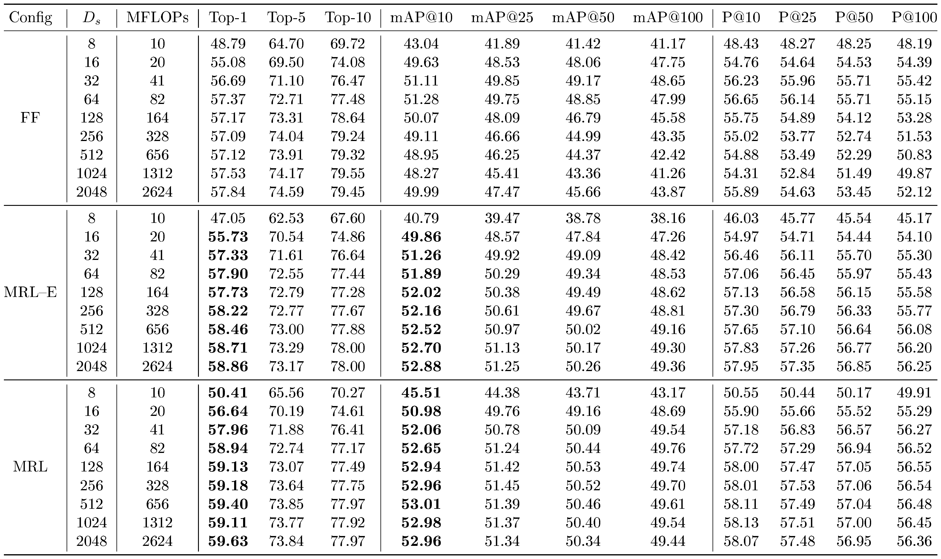
We examined the robustness of ${\rm MRL}$ for retrieval on out-of-domain datasets ImageNetV2 and ImageNet-4K, as shown in Table 9 and Table 10 respectively. On ImageNetV2, we observed that ${\rm MRL}$ outperformed FF at all $D_s$ on top-1 Accuracy and mAP@10, and MRL–E outperformed FF at all $D_s$ except $D_s$ $ = 8$. This demonstrates the robustness of the learned ${\rm Matryoshka~Representations}$ for out-of-domain image retrieval.

F. Adaptive Retrieval

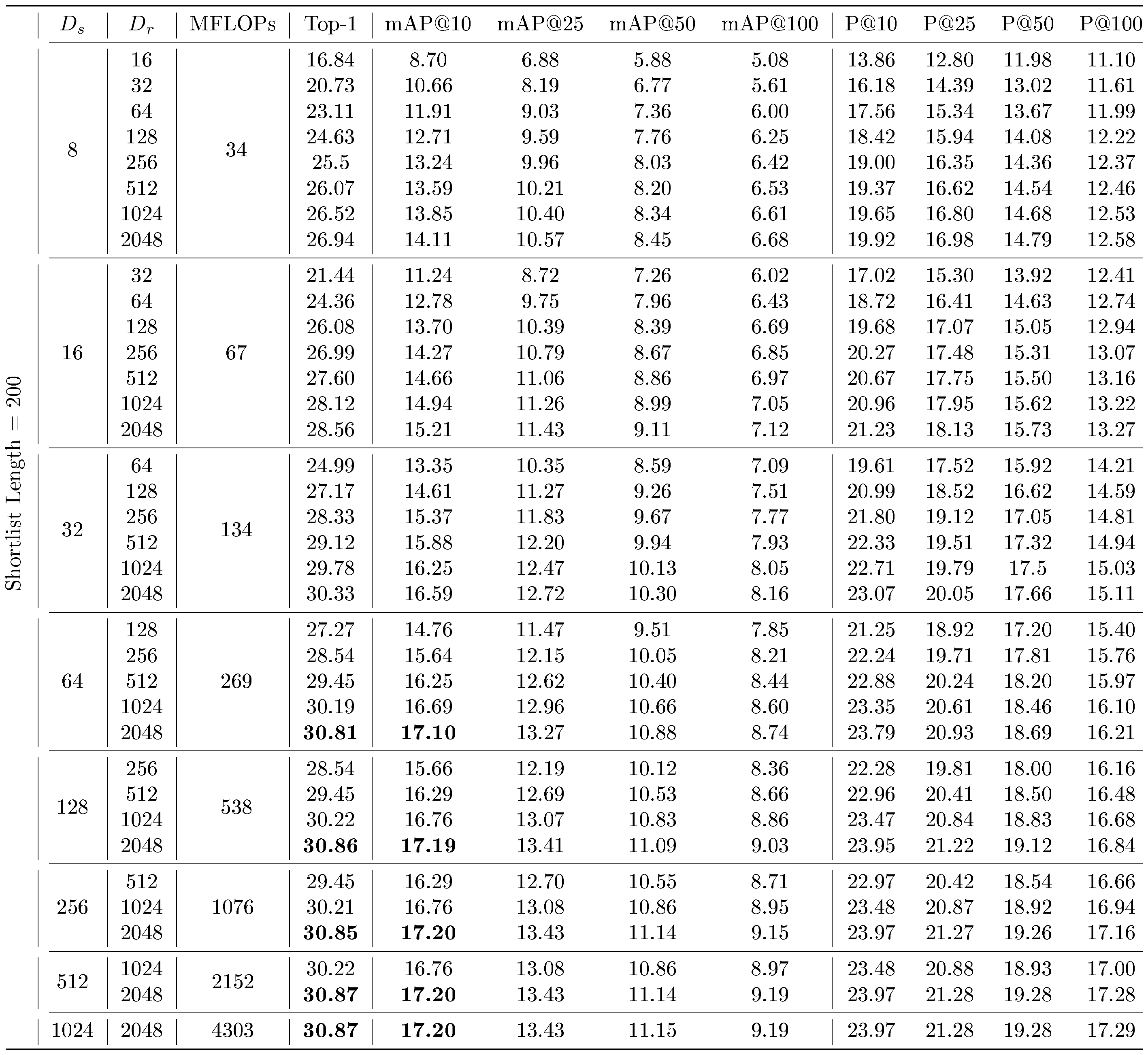
The time complexity of retrieving a shortlist of k-NN often scales as $O(d)$, where $d = $ $D_s$, for a fixed k and $N$. We thus will have a theoretical $256\times$ higher cost for $D_s$ $ = 2048$ over $D_s$ $ = 8$. We discuss search complexity in more detail in Appendix I. In an attempt to replicate performance at higher $D_s$ while using less FLOPs, we perform adaptive retrieval via retrieving a k-NN shortlist with representation size $D_s$, and then re-ranking the shortlist with representations of size $D_r$ . Adaptive retrieval for a shortlist length $k = 200$ is shown in Table 11 for ImageNet-1K, and in Table 12 for ImageNet-4K. On ImageNet-1K, we are able to achieve comparable performance to retrieval with $D_s$ $ = 2048$ (from Table 8) with $D_s$ $= 16$ at $128\times$ less MFLOPs/Query (used interchangeably with MFLOPs). Similarly, on ImageNet-4K, we are able to achieve comparable performance to retrieval with $D_s$ $ = 2048$ (from Table 10) with $D_s$ $ = 64$ on ImageNet-1K and ImageNet-4K, at $32\times$ less MFLOPs. This demonstrates the value of intelligent routing techniques which utilize appropriately sized Matryoshka Representations for retrieval.

::: {caption="Table 11: Retrieve a shortlist of k-NN with $D_s$ sized representations on ImageNet-1K with MRL representations, and then re-order the neighbors shortlist with L2 distances using $D_r$ sized representations. Top-1 and mAP@10 entries (%) that are within $0.1%$ of the maximum value achievable without reranking on MRL representations, as seen in Table 8, are bolded."}

:::

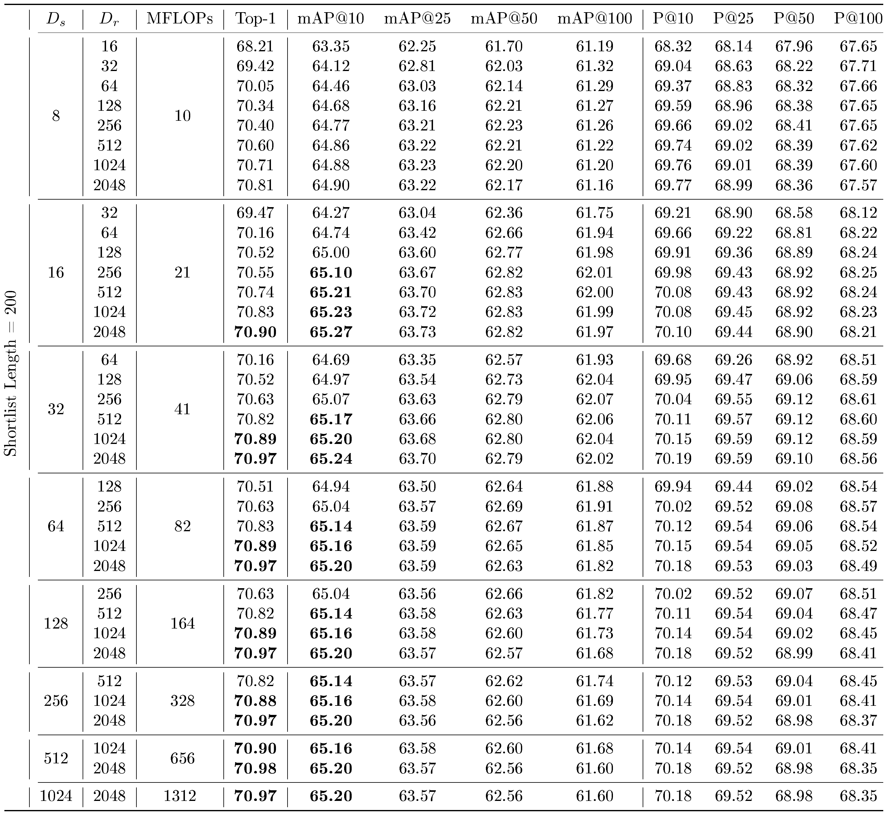
::: {caption="Table 12: Retrieve a shortlist of k-NN with $D_s$ sized representations on ImageNet-4K with MRL representations, and then re-order the neighbors shortlist with L2 distances using $D_r$ sized representations. Top-1 and mAP@10 entries (%) that are within $0.1%$ of the maximum value achievable without reranking on MRL representations, as seen in Table 10, are bolded."}

:::

Funnel Retrieval.

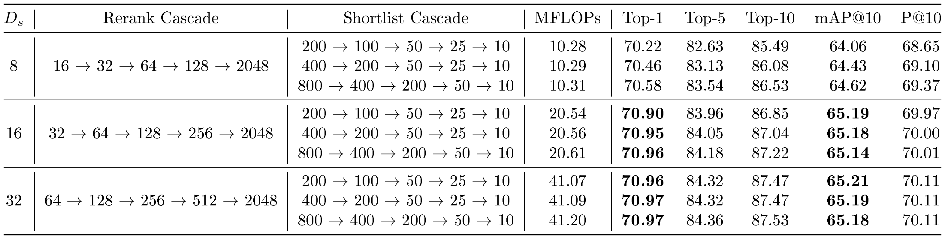
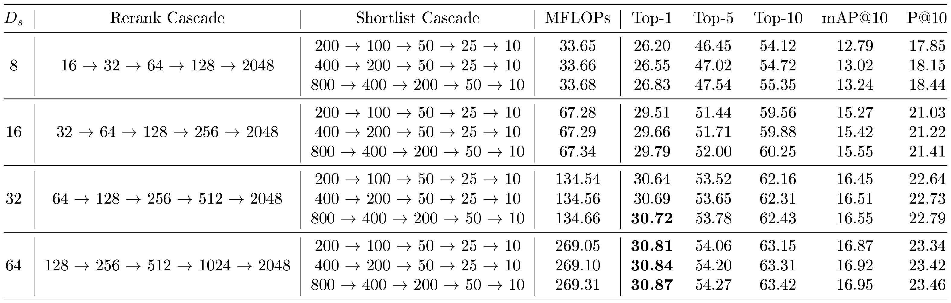
We also designed a simple cascade policy which we call funnel retrieval to successively improve and refine the k-NN shortlist at increasing $D_s$ . This was an attempt to remove the dependence on manual choice of $D_s$ & $D_r$ . We retrieved a shortlist at $D_s$ and then re-ranked the shortlist five times while simultaneously increasing $D_r$ (rerank cascade) and decreasing the shortlist length (shortlist cascade), which resembles a funnel structure. We tabulate the performance of funnel retrieval in various configurations in Table 13 on ImageNet-1K, and in Table 14 on ImageNet-4K. With funnel retrieval on ImageNet-1K, we were able to achieve top-1 accuracy within $0.1%$ of retrieval with $D_s$ $= 2048$ (as in Table 8) with a funnel with $D_s$ $ = 16$, with $128\times$ less MFLOPs. Similarly, we are able to achieve equivalent top-1 accuracy within $0.15%$ of retrieval at $D_s$ $ = 2048$ (as in Table 10) with funnel retrieval at $D_s$ $ = 32$ on ImageNet-4K, with $64\times$ less MFLOPs. This demonstrates that with funnel retrieval, we can emulate the performance of retrieval with $D_s$ $ = 2048$ with a fraction of the MFLOPs.

::: {caption="Table 13: Retrieve a shortlist of k-NN with $D_s$ sized representations on ImageNet-1K with MRL. This shortlist is then reranked with funnel retrieval, which uses a rerank cascade with a one-to-one mapping with a monotonically decreasing shortlist length as shown in the shortlist cascade. Top-1 and mAP@10 entries (%) within $0.1%$ of the maximum achievable without reranking on MRL representations, as seen in Table 8, are bolded."}

:::

::: {caption="Table 14: Retrieve a shortlist of k-NN with $D_s$ sized representations on ImageNet-4K with MRL. This shortlist is then reranked with funnel retrieval, which uses a rerank cascade with a one-to-one mapping with a monotonically decreasing shortlist length as shown in the shortlist cascade. Top-1 and mAP@10 entries (%) within $0.15%$ of the maximum achievable without reranking on MRL representations, as seen in Table 10, are bolded."}

:::

G. Few-shot and Sample Efficiency

We compared MRL, MRL–E, and FF on various benchmarks to observe the effect of representation size on sample efficiency. We used Nearest Class Means [83] for classification which has been shown to be effective in the few-shot regime [101].

ImageNetV2.

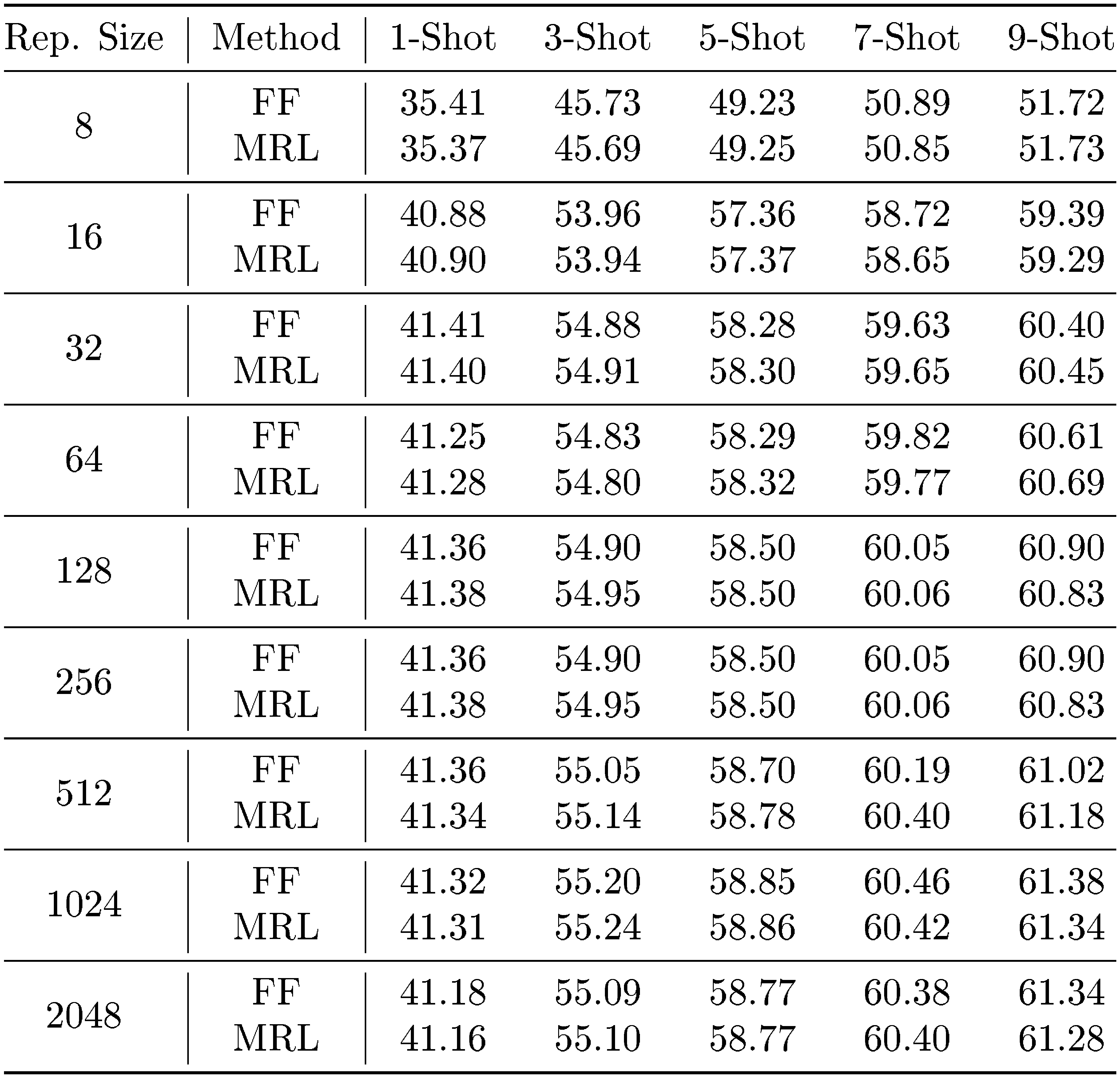
Representations are evaluated on ImageNetV2 with the n-shot k-way setup. ImageNetV2 is a dataset traditionally used to evaluate the robustness of models to natural distribution shifts. For our experiments we evaluate accuracy of the model given $n$ examples from the ImageNetV2 distribution. We benchmark representations in the traditional small-scale (10-way) and large-scale (1000-way) setting. We evaluate for $n \in 1, 3, 5, 7, 9$ with 9 being the maximum value for $n$ because there are 10 images per class.

We observed that MRL had equal performance to FF across all representation sizes and shot numbers. We also found that for both MRL and FF, as the shot number decreased, the required representation size to reach optimal accuracy decreased (Table 15). For example, we observed that 1-shot performance at $32$ representation size had equal accuracy to $2048$ representation size.

::: {caption="Table 15: Few-shot accuracy (%) on ImageNetV2 for 1000-way classification. MRL performs equally to FF across all shots and representation sizes. We also observed that accuracy saturated at a lower dimension for lower shot numbers. E.g. for 1-shot, 32-dim performed comparably to 2048-dim."}

:::

FLUID.

For the long-tailed setting we evaluated MRL on the FLUID benchmark ([84]) which contains a mixture of pretrain and new classes. Table 16 shows the evaluation of the learned representation on FLUID. We observed that MRL provided up to 2% higher accuracy on novel classes in the tail of the distribution, without sacrificing accuracy on other classes. Additionally we found the accuracy between low-dimensional and high-dimensional representations was marginal for pretrain classes. For example, the 64-dimensional MRL performed $\sim1%$ lower in accuracy compared to the 2048-dimensional counterpart on pretrain-head classes (84.46% vs 85.60%). However for novel-tail classes the gap was far larger (6.22% vs 12.88%). We hypothesize that the higher-dimensional representations are required to differentiate the classes when few training examples of each are known. These results provide further evidence that different tasks require varying capacity based on their difficulty.

::: {caption="Table 16: Accuracy (%) categories indicates whether classes were present during ImageNet pretraining and head/tail indicates classes that have greater/less than 50 examples in the streaming test set. We observed that MRL performed better than the baseline on novel tail classes by $\sim2%$ on average."}

:::

H. Robustness Experiments

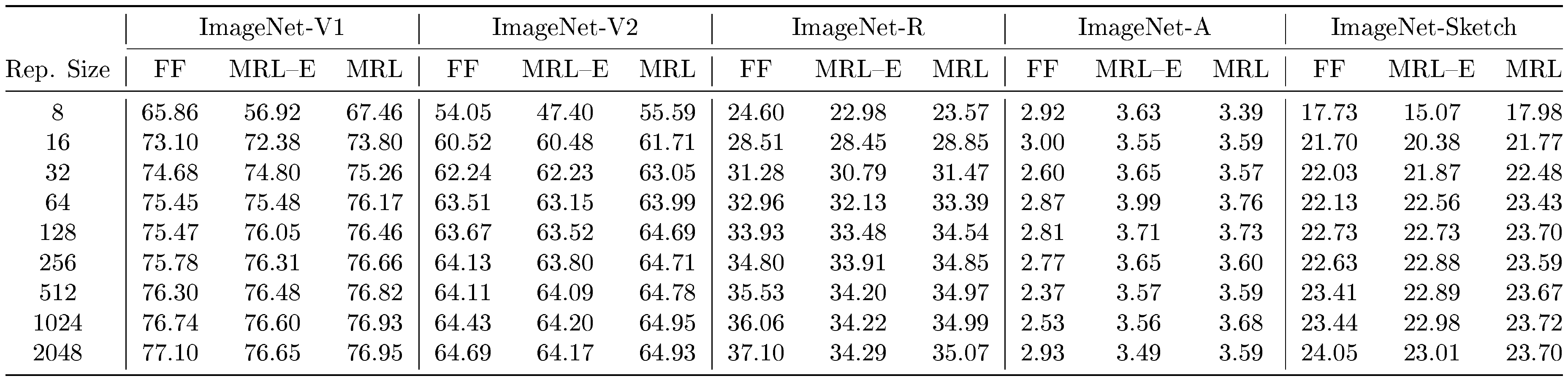
::: {caption="Table 17: Top-1 classification accuracy (%) on out-of-domain datasets (ImageNet-V2/R/A/Sketch) to examine robustness of Matryoshka Representation Learning. Note that these results are without any fine tuning on these datasets."}

:::

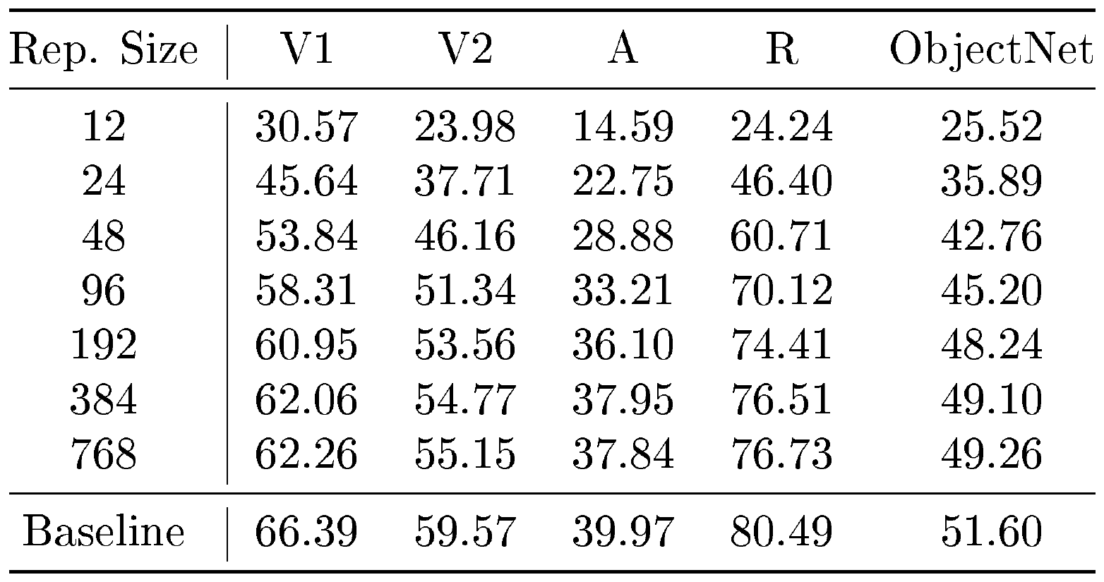
::: {caption="Table 18: Zero-shot top-1 image classification accuracy (%) of a ALIGN- MRL model on ImageNet-V1/V2/R/A and ObjectNet."}

:::

We evaluated the robustness of MRL models on out-of-domain datasets (ImageNetV2/R/A/Sketch) and compared them to the FF baseline. Each of these datasets is described in Appendix B. The results in Table 17 demonstrate that learning Matryoshka Representations does not hurt out-of-domain generalization relative to FF models, and Matryoshka Representations in fact improve the performance on ImageNet-A. For a ALIGN– MRL model, we examine the the robustness via zero-shot retrieval on out-of-domain datasets, including ObjectNet, in Table 18.

I. In Practice Costs

All approximate NN search experiments via HNSW32 were run on an Intel Xeon 2.20GHz CPU with 24 cores. All exact search experiments were run with CUDA 11.0 on 2xA100-SXM4 NVIDIA GPUs with 40G RAM each.

MRL models.

As MRL makes minimal modifications to the ResNet50 model in the final fc layer via multiple heads for representations at various scales, it has only an 8MB storage overhead when compared to a standard ResNet50 model. MRL–E has no storage overhead as it has a shared head for logits at the final fc layer.

Retrieval

Exact search has a search time complexity of $O(dkN)$, and HNSW has a search time complexity of $O(dk\log(N))$, where $N$ is the database size, $d$ is the representation size, and $k$ is the shortlist length. To examine real-world performance, we tabulated wall clock search time for every query in the ImageNet-1K and ImageNet-4K validation sets over all representation sizes $d$ in Table 19 for both Exact Search and HNSW32, and ablated wall clock query time over shortlist length $k$ on the ImageNet-1K validation set in Table 21. The wall clock time to build the index and the index size is also shown in Table 20.

::: {caption="Table 19: Retrieval k-NN wall clock search times (s) over the entire validation (query) set of ImageNet-1K and ImageNet-4K, containing 50K and 200K samples respectively."}

:::

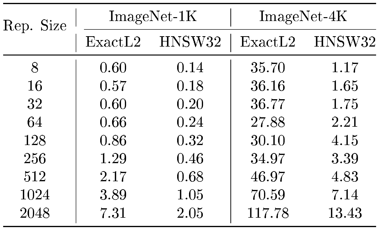
::: {caption="Table 20: FAISS ([100]) index size and build times for exact k-NN search with L2 Distance metric and approximate k-NN search with HNSW32 ([48])."}

:::

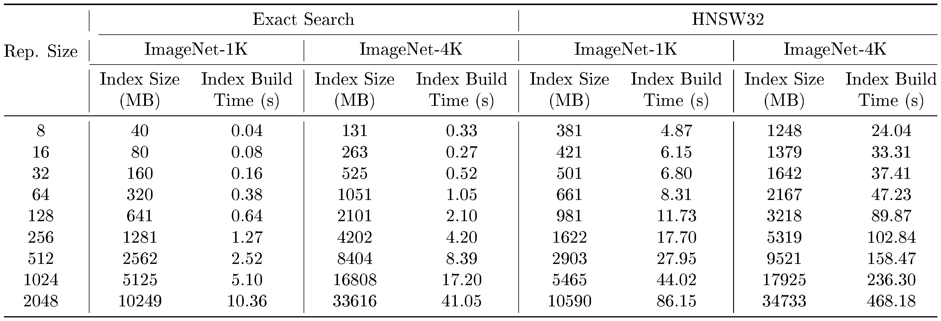
: Table 21: Retrieval k-NN wall clock search times (s) over entire validation (query) set of ImageNet-1K over various shortlist lengths $k$.

Index	k = 50	k = 100	k = 200	k = 500	k = 1000	k = 2048
Exact L2	0.4406	0.4605	0.5736	0.6060	1.2781	2.7047
HNSW32	0.1193	0.1455	0.1833	0.2145	0.2333	0.2670

J. Analysis of Model Disagreement

Class Trends

Does increasing representation size necessarily help improve classification performance across all classes in ImageNet-1K? We studied this question by examining trends in performance with increasing representation size from $d = 8, ... 2048$. For MRL models, we observed that $244$ classes showed a monotonic improvement in performance with increasing $d$, $177$ classes first improved but then observed a slight dip (one or two misclassifications per class), $49$ classes showed a decline first and then an improvement, and the remaining classes did not show a clear trend. When we repeated this experiment with independently trained FF models, we noticed that $950$ classes did not show a clear trend. This motivated us to leverage the disagreement as well as gradual improvement of accuracy at different representation sizes by training Matryoshka Representations. Figure 15 showcases the progression of relative per-class accuracy distribution compared to the Matryoshka Representation Learning-2048 dimensional model. This also showed that some instances and classes could benefit from lower-dimensional representations.

Discussion of Oracle Accuracy

Based on our observed model disagreements for different representation sizes $d$, we defined an optimal oracle accuracy ([102]) for MRL. We labeled an image as correctly predicted if classification using any representation size was correct. The percentage of total samples of ImageNet-1K that were firstly correctly predicted using each representation size $d$ is shown in Table 22. This defined an upper bound on the performance of MRL models, as $18.46%$ of the ImageNet-1K validation set were incorrectly predicted $\forall d\in{8, 16, \ldots, 2048}$. We show the oracle performance on MRL models for ImageNet-1K/V2/A/R/Sketch datasets in Table 23.

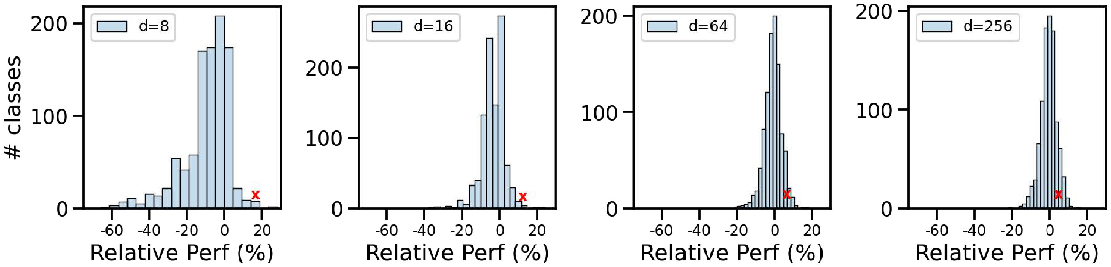
In an attempt to derive an optimal routing policy to emulate oracle accuracy, we designed the adaptive classification via cascading method as discussed in Appendix D.1. This led to an interesting observation on the expected dimensionality for $76.30%$ top-1 classification accuracy being just $d \sim37$. We leave the design and learning of a more optimal policy for future work.

::: {caption="Table 22: Percentage of ImageNet-1K validation set that is first correctly predicted using each representation size $d$. We note that $18.46%$ of the samples cannot be correctly predicted by any representation size. The remaining $81.54%$ constitutes the oracle accuracy."}

:::

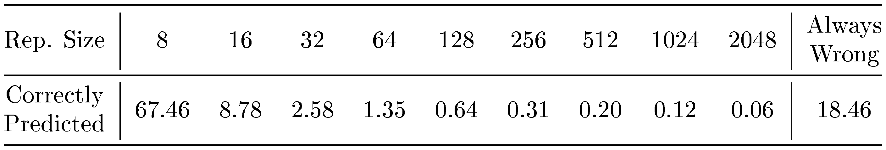
: Table 23: Oracle classification accuracy of various evaluation datasets for ResNet50– MRL model trained on ImageNet-1K.

Top-1	ImageNetV1	ImageNetV2	ImageNet-A	ImageNet-R	ImageNet-Sketch
FF–2048	76.9	64.9	3.6	35.1	23.7
MRL–Oracle	81.5	70.6	8.7	39.8	28.9

Grad-CAM Examples

We analyzed the nature of model disagreement across representation sizes with MRL models with the help of Grad-CAM visualization ([85]). We observed there were certain classes in ImageNet-1K such as "tools", "vegetables" and "meat cutting knife" which were occasionally located around multiple objects and a cluttered environment. In such scenarios, we observed that smaller representation size models would often get confused due to other objects and fail to extract the object of interest which generated the correct label. We also observed a different nature of disagreement arising when the models got confused within the same superclass. For example, ImageNet-1K has multiple "snake" classes, and models often confuse a snake image for an incorrect species of snake.

Superclass Performance

We created a 30 superclass subset of the validation set based on wordnet hierarchy (Table 24) to quantify the performance of MRL model on ImageNet-1K superclasses. Table 25 quantifies the performance with different representation size.

: Table 24: 30 Superclasses in ImageNet-1K corresponding to the performance in Table 25.

insect	motor vehicle	artiodactyl	vegetable	game equipment
terrier	serpent	machine	measuring device	sheepdog
protective covering	sporting dog	vessel, watercraft	building	lizard
garment	hound	monkey	home appliance	wind instrument
vessel	fish	nourishment	electronic equipment	oscine
furniture	wading bird	tool	canine	mechanism

: Table 25: Performance of MRL model on 31-way classification (1 extra class is for reject token) on ImageNet-1K superclasses.

Rep. Size	8	16	32	64	128	256	512	1024	2048
MRL	85.57	88.67	89.48	89.82	89.97	90.11	90.18	90.22	90.21

K. Ablation Studies

K.1 MRL Training Paradigm

::: {caption="Table 26: Top-1 classification accuracy (%) on ImageNet-1K of various ResNet50 models which are finetuned on pretrained FF-2048 model. We observed that adding more non-linearities is able to induce nesting to a reasonable extent even if the model was not pretrained with nesting in mind."}

:::

Matryoshka Representations via Finetuning.

To observe if nesting can be induced in models that were not explicitly trained with nesting from scratch, we loaded a pretrained FF-2048 ResNet50 model and initialized a new MRL layer, as defined in Algorithm 2, Appendix C. We then unfroze different layers of the backbone to observe how much non-linearity in the form of unfrozen conv layers needed to be present to enforce nesting into a pretrained FF model. A description of these layers can be found in the ResNet50 architecture [5]. All models were finetuned with the FFCV pipeline, with same training configuration as in the end-to-end training aside from changing lr $ = 0.1$ and epochs $ = 10$. We observed that finetuning the linear layer alone was insufficient to learn Matryoshka Representations at lower dimensionalities. Adding more and more non-linear conv+ReLU layers steadily improved classification accuracy of $d = 8$ from $5%$ to $60%$ after finetuning, which was only $6%$ less than training MRL end-to-end for 40 epochs. This difference was successively less pronounced as we increased dimensionality past $d = 64$, to within $1.5%$ for all larger dimensionalities. The full results of this ablation can be seen in Table 26.

::: {caption="Table 27: An ablation over boosting training loss at lower nesting dimensions, with top-1 and top-5 accuracy (%). The models are described in Appendix K.1."}

:::

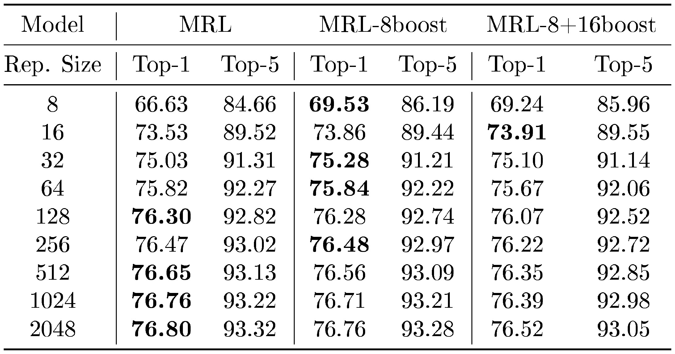
Relative Importance.

We performed an ablation of MRL over the relative importance, $c_m$, of different nesting dimensions $m\in\cal{M}$, as defined in Section 3. In an attempt to improve performance at lower dimensionalities, we boosted the relative importance $c_m$ of training loss at lower dimensions as in Equation 1 with two models, MRL-8boost and MRL-8+16boost. The MRL-8boost model had $c_{m\in\cal M} = [2, 1, 1, 1, 1, 1, 1, 1, 1]$ and the MRL-8+16boost model had $c_{m\in\cal M} = [2, 1.5, 1, 1, 1, 1, 1, 1, 1]$. The relative importance list $c_{m\in\cal M}$ had a 1-to-1 correspondence with nesting dimension set $\mathcal{M}$. In Table 27, we observed that MRL-8boost improves top-1 accuracy by $3%$ at $d = 8$, and also improves top-1 accuracy of all representation scales from 16 to 256 over MRL, while only hurting the performance at 512 to 2048 representation scales by a maximum of 0.1%. This suggests that the relative importance $c_m$ can be tuned/set for optimal accuracy for all $m\in\mathcal{M}$, but we leave this extension for future work.

Matryoshka Representations at Arbitrary Granularities.

To train MRL, we used nested dimensions at logarithmic granularities $\mathcal{M} = {8, 16, \ldots, 1024, 2048}$ as detailed in Section 3. We made this choice for two empirically-driven reasons: a) The accuracy improvement with increasing representation size was more logarithmic than linear (as shown by FF models in Figure 5). This indicated that optimizing for granularities increasing in a non-logarithmic fashion would be sub-optimal both for maximum performance and expected efficiency; b) If we have $m$ arbitrary granularities, the expected cost of the linear classifier to train MRL scales as $O(L*(m^2))$ while logarithmic granularities result in $O(L*2log(d))$ space and compute costs.

To demonstrate this effect, we learned Matryoshka Representations with uniform (MRL-Uniform) nesting dimensions $m\in\mathcal{M} = {8, 212, 416, 620, 824, 1028, 1232, 1436, 1640, 1844, 2048}$. We evaluated this model at the standard (MRL-log) dimensions $m\in\mathcal{M} = {8, 16, 32, 64, 128, 256, 512, 1024, 2048}$ for ease of comparison to reported numbers using 1-NN accuracy (%). As shown in Table 29, we observed that while performance interpolated, MRL-Uniform suffered at low dimensions as the logarithmic spacing of MRL-log resulted in tighter packing of information in these initial dimensions. The higher nesting dimensions of MRL-Uniform did not help in significant accuracy improvement due to accuracy saturation, which is often logarithmic in representation size as shown by FF models. Note that the slight improvement at dimensions higher than 512 for MRL-Uniform is due to multiple granularities around them compared to just three for MRL-log, which are not useful in practice for efficiency.

Lower Dimensionality.

We experimented with training MRL with smaller nesting dimension than $m = 8$, as shown in Table 28, with two models: MRL-4 and MRL-6. We found that using lower than 8-dimensions to train MRL, i.e. $m_0 \in {4, 6}$ for MRL-4 and MRL-6 respectively, did not affect the top-1 accuracy of other granularities significantly. However, granularities smaller than 8-dimensions had very low accuracy and were often unusable for deployment along with additional training difficulty. We also observed a small dip in accuracy at higher dimensions which we attribute to the joint loss that now also included the harder optimization of the smallest dimension. Lastly, we hypothesize the dimensionality of 8 is an empirically validated design choice due to the considerable accuracy it provided along with the ease of training.

\begin{tabular}{@c|ccc@}
\toprule
Rep. Size & MRL-4 & MRL-6 & MRL-8 \\ \midrule
4 & 27.25 & - & - \\
6 & - & 58.71 & - \\
8 & 66.86 & \textbf{67.55} & 66.63 \\
16 & 73.36 & 73.10 & \textbf{73.53} \\
32 & 74.82 & 74.49 & \textbf{75.03} \\
64 & 75.51 & 75.32 & \textbf{75.82} \\
128 & 75.93 & 75.61 & \textbf{76.30} \\
256 & 76.08 & 75.82 & \textbf{76.47} \\
512 & 76.31 & 75.93 & \textbf{76.65} \\
1024 & 76.38 & 76.04 & \textbf{76.76} \\
2048 & 76.43 & 76.12 & \textbf{76.80} \\ \bottomrule
\end{tabular}

\begin{tabular}{@c|cc@}
\toprule
Rep. Size & {\rm MRL}-Log & {\rm MRL}-Uniform \\ \midrule
8 & \textbf{62.19} & 58.44 \\
16 & \textbf{67.91} & 61.11 \\
32 & \textbf{69.46} & 63.82 \\
64 & \textbf{70.17} & 66.44 \\
128 & \textbf{70.52} & 68.71 \\
256 & \textbf{70.62} & 70.06 \\
512 & 70.82 & \textbf{70.98} \\
1024 & 70.89 & \textbf{71.37} \\
2048 & 70.97 & \textbf{71.44} \\ \bottomrule
\end{tabular}

K.2 Retrieval

Adaptive Retrieval.

To examine the effect of increasing shortlist lengths on search time, we performed a reranking ablation over shortlist lengths for $D_s$ = 16 and $D_r$ = 2048 over ImageNet-1K in Table 30, and over ImageNet-4K in Table 31. We observed that using a larger shortlist $k$ saturated ImageNet-1K performance at $k$ =200. But using larger shortlists until $k=2048$, the maximum value supported by the FAISS framework, steadily improved performance on ImageNet-4K. This is likely due to the increased database size, but could also indicate a correlation with ImageNet-4K being slightly out-of-distribution making the task at hand harder.

::: {caption="Table 30: Adaptive retrieval ablation over shortlist length $k$ for $D_s = 16$, $D_r = 2048$ on ImageNet-1K with exact search. Entries with the highest P@1 and mAP@10 across all $k$ are in bold."}

:::

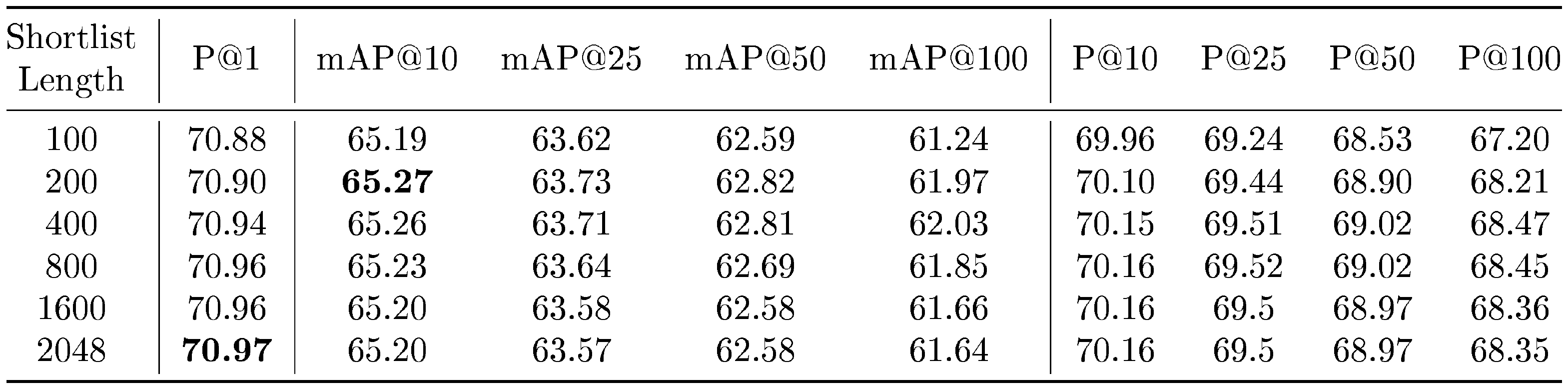
::: {caption="Table 31: Adaptive retrieval ablation over shortlist length $k$ for $D_s = 16$, $D_r = 2048$ on ImageNet-4K with exact search."}

:::

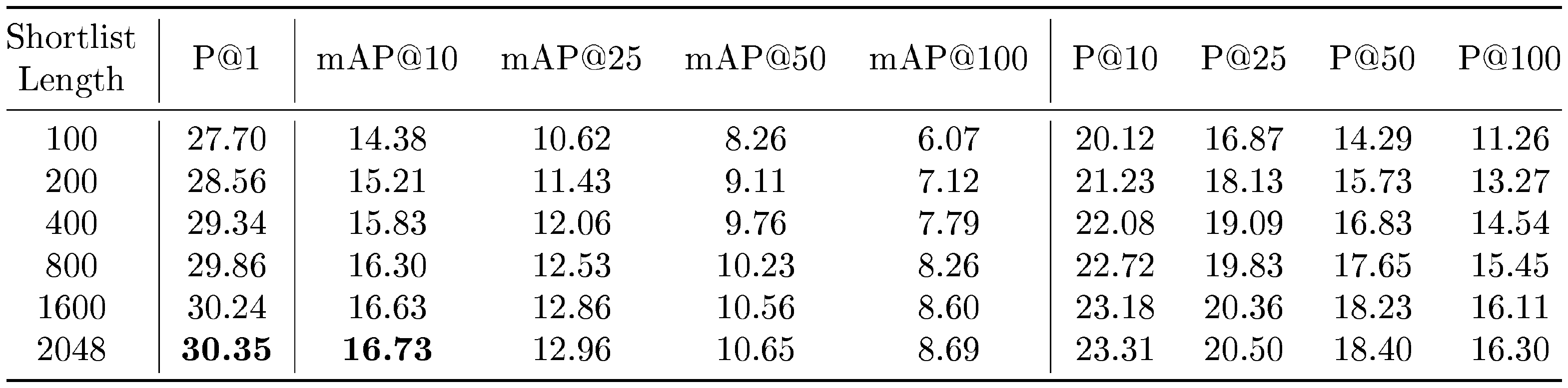
References

[1] LeCun et al. (2015). Deep learning. nature. 521(7553). pp. 436–444.

[2] Pandu Nayak (2019). Understanding searches better than ever before. Google AI Blog. https://blog.google/products/search/search-language-understanding-bert/.

[3] Charlie Waldburger (2019). As search needs evolve, Microsoft makes AI tools for better search available to researchers and developers. Microsoft AI Blog. https://blogs.microsoft.com/ai/bing-vector-search/.

[4] Bengio, Yoshua (2012). Deep learning of representations for unsupervised and transfer learning. In Proceedings of ICML workshop on unsupervised and transfer learning. pp. 17–36.

[5] He et al. (2016). Deep residual learning for image recognition. In Proceedings of the IEEE conference on computer vision and pattern recognition. pp. 770–778.

[6] Kaz Sato, Tomoyuki Chikanaga (2021). Vertex AI Matching Engine. Microsoft AI Blog. https://cloud.google.com/blog/topics/developers-practitioners/find-anything-blazingly-fast-googles-vector-search-technology.

[7] Varma, Manik (2019). Extreme classification. Communications of the ACM. 62(11). pp. 44–45.

[8] Dean, Jeffrey (2009). Challenges in building large-scale information retrieval systems. In Keynote of the 2nd ACM International Conference on Web Search and Data Mining (WSDM).

[9] Sun et al. (2017). Revisiting unreasonable effectiveness of data in deep learning era. In Proceedings of the IEEE international conference on computer vision. pp. 843–852.

[10] Harris, Mike G and Giachritsis, Christos D (2000). Coarse-grained information dominates fine-grained information in judgments of time-to-contact from retinal flow. Vision research. 40(6). pp. 601–611.

[11] Hegdé, Jay (2008). Time course of visual perception: coarse-to-fine processing and beyond. Progress in neurobiology. 84(4). pp. 405–439.

[12] Soudry et al. (2018). The implicit bias of gradient descent on separable data. The Journal of Machine Learning Research. 19(1). pp. 2822–2878.

[13] Cai et al. (2019). Once-for-all: Train one network and specialize it for efficient deployment. arXiv preprint arXiv:1908.09791.

[14] Yu et al. (2018). Slimmable neural networks. arXiv preprint arXiv:1812.08928.

[15] Hotelling, Harold (1933). Analysis of a complex of statistical variables into principal components.. Journal of educational psychology. 24(6). pp. 417.

[16] Linde et al. (1980). An algorithm for vector quantizer design. IEEE Transactions on communications. 28(1). pp. 84–95.

[17] Deng et al. (2009). Imagenet: A large-scale hierarchical image database. In 2009 IEEE conference on computer vision and pattern recognition. pp. 248–255.

[18] Russakovsky et al. (2015). Imagenet large scale visual recognition challenge. International journal of computer vision. 115(3). pp. 211–252.

[19] Yosinski et al. (2014). How transferable are features in deep neural networks?. Advances in neural information processing systems. 27.

[20] Krizhevsky et al. (2012). Imagenet classification with deep convolutional neural networks. Advances in neural information processing systems. 25.

[21] Simonyan, Karen and Zisserman, Andrew (2014). Very deep convolutional networks for large-scale image recognition. arXiv preprint arXiv:1409.1556.

[22] Wu et al. (2018). Unsupervised feature learning via non-parametric instance-level discrimination. arXiv preprint arXiv:1805.01978.

[23] He et al. (2021). Masked autoencoders are scalable vision learners. arXiv preprint arXiv:2111.06377.

[24] Masci et al. (2011). Stacked convolutional auto-encoders for hierarchical feature extraction. In International conference on artificial neural networks. pp. 52–59.

[25] Chen et al. (2020). A simple framework for contrastive learning of visual representations. In International conference on machine learning. pp. 1597–1607.

[26] He et al. (2020). Momentum contrast for unsupervised visual representation learning. In Proceedings of the IEEE/CVF conference on computer vision and pattern recognition. pp. 9729–9738.

[27] Gutmann, Michael and Hyvärinen, Aapo (2010). Noise-contrastive estimation: A new estimation principle for unnormalized statistical models. In Proceedings of the thirteenth international conference on artificial intelligence and statistics. pp. 297–304.

[28] Divvala et al. (2014). Learning everything about anything: Webly-supervised visual concept learning. In Proceedings of the IEEE Conference on Computer Vision and Pattern Recognition. pp. 3270–3277.

[29] Desai, Karan and Johnson, Justin (2021). Virtex: Learning visual representations from textual annotations. In Proceedings of the IEEE/CVF Conference on Computer Vision and Pattern Recognition. pp. 11162–11173.

[30] Jia et al. (2021). Scaling up visual and vision-language representation learning with noisy text supervision. In International Conference on Machine Learning. pp. 4904–4916.

[31] Radford et al. (2021). Learning transferable visual models from natural language supervision. In International Conference on Machine Learning. pp. 8748–8763.

[32] Zellers et al. (2022). MERLOT Reserve: Neural Script Knowledge through Vision and Language and Sound. arXiv preprint arXiv:2201.02639.

[33] Howard, Jeremy and Ruder, Sebastian (2018). Universal language model fine-tuning for text classification. arXiv preprint arXiv:1801.06146.

[34] Brown et al. (2020). Language models are few-shot learners. Advances in neural information processing systems. 33. pp. 1877–1901.

[35] Peters et al. (2018). Deep Contextualized Word Representations. In Proceedings of the 2018 Conference of the North American Chapter of the Association for Computational Linguistics: Human Language Technologies, Volume 1 (Long Papers). pp. 2227–2237. doi:10.18653/v1/N18-1202. https://aclanthology.org/N18-1202.

[36] Ruder et al. (2019). Transfer learning in natural language processing. In Proceedings of the 2019 conference of the North American chapter of the association for computational linguistics: Tutorials. pp. 15–18.

[37] Devlin et al. (2018). Bert: Pre-training of deep bidirectional transformers for language understanding. arXiv preprint arXiv:1810.04805.

[38] Radford et al. (2018). Improving language understanding by generative pre-training. OpenAI Blog. https://openai.com/blog/language-unsupervised/.

[39] Gholami et al. (2021). A survey of quantization methods for efficient neural network inference. arXiv preprint arXiv:2103.13630.

[40] Kusupati et al. (2020). Soft threshold weight reparameterization for learnable sparsity. In International Conference on Machine Learning. pp. 5544–5555.

[41] Howard et al. (2017). Mobilenets: Efficient convolutional neural networks for mobile vision applications. arXiv preprint arXiv:1704.04861.

[42] Kusupati et al. (2018). Fastgrnn: A fast, accurate, stable and tiny kilobyte sized gated recurrent neural network. Advances in Neural Information Processing Systems. 31.

[43] Tan, Mingxing and Le, Quoc (2019). Efficientnet: Rethinking model scaling for convolutional neural networks. In International conference on machine learning. pp. 6105–6114.

[44] Bengio et al. (2010). Label embedding trees for large multi-class tasks. Advances in Neural Information Processing Systems. 23.

[45] Jain et al. (2019). Slice: Scalable linear extreme classifiers trained on 100 million labels for related searches. In Proceedings of the Twelfth ACM International Conference on Web Search and Data Mining. pp. 528–536.

[46] Prabhu et al. (2020). Extreme regression for dynamic search advertising. In Proceedings of the 13th International Conference on Web Search and Data Mining. pp. 456–464.

[47] Dietterich, Thomas G and Bakiri, Ghulum (1994). Solving multiclass learning problems via error-correcting output codes. Journal of artificial intelligence research. 2. pp. 263–286.

[48] Malkov, Yu A and Yashunin, Dmitry A (2018). Efficient and robust approximate nearest neighbor search using hierarchical navigable small world graphs. IEEE transactions on pattern analysis and machine intelligence. 42(4). pp. 824–836.

[49] Deng et al. (2011). Hierarchical semantic indexing for large scale image retrieval. In CVPR 2011. pp. 785–792.

[50] Kusupati et al. (2021). LLC: Accurate, Multi-purpose Learnt Low-dimensional Binary Codes. Advances in Neural Information Processing Systems. 34.

[51] Salakhutdinov, Ruslan and Hinton, Geoff (2007). Learning a nonlinear embedding by preserving class neighbourhood structure. In Artificial Intelligence and Statistics. pp. 412–419.

[52] Van Der Maaten et al. (2009). Dimensionality reduction: a comparative. J Mach Learn Res. 10(66-71). pp. 13.

[53] Datar et al. (2004). Locality-sensitive hashing scheme based on p-stable distributions. In Proceedings of the twentieth annual symposium on Computational geometry. pp. 253–262.

[54] Kulis et al. (2009). Fast similarity search for learned metrics. IEEE Transactions on Pattern Analysis and Machine Intelligence. 31(12). pp. 2143–2157.

[55] Salakhutdinov, Ruslan and Hinton, Geoffrey (2009). Semantic hashing. International Journal of Approximate Reasoning. 50(7). pp. 969–978.

[56] Mitra et al. (2002). Unsupervised feature selection using feature similarity. IEEE transactions on pattern analysis and machine intelligence. 24(3). pp. 301–312.

[57] Chang et al. (2021). Extreme multi-label learning for semantic matching in product search. In Proceedings of the 27th ACM SIGKDD Conference on Knowledge Discovery & Data Mining. pp. 2643–2651.

[58] Chang et al. (2020). Pre-training tasks for embedding-based large-scale retrieval. arXiv preprint arXiv:2002.03932.

[59] Yu et al. (2022). PECOS: Prediction for enormous and correlated output spaces. Journal of Machine Learning Research. 23(98). pp. 1–32.

[60] Brin, Sergey and Page, Lawrence (1998). The anatomy of a large-scale hypertextual web search engine. Computer networks and ISDN systems. 30(1-7). pp. 107–117.

[61] Indyk, Piotr and Motwani, Rajeev (1998). Approximate nearest neighbors: towards removing the curse of dimensionality. In Proceedings of the thirtieth annual ACM symposium on Theory of computing. pp. 604–613.

[62] Bentley, Jon Louis (1990). K-d trees for semidynamic point sets. In Proceedings of the sixth annual symposium on Computational geometry. pp. 187–197.

[63] Beygelzimer et al. (2006). Cover trees for nearest neighbor. In Proceedings of the 23rd international conference on Machine learning. pp. 97–104.

[64] Jayaram Subramanya et al. (2019). Diskann: Fast accurate billion-point nearest neighbor search on a single node. Advances in Neural Information Processing Systems. 32.

[65] Wallingford et al. (2022). Task Adaptive Parameter Sharing for Multi-Task Learning. arXiv preprint arXiv:2203.16708.

[66] Engelsma et al. (2022). HERS: Homomorphically encrypted representation search. IEEE Transactions on Biometrics, Behavior, and Identity Science. 4(3). pp. 349–360.

[67] Gong et al. (2019). On the intrinsic dimensionality of image representations. In Proceedings of the IEEE/CVF Conference on Computer Vision and Pattern Recognition. pp. 3987–3996.

[68] Nanda et al. (2023). Diffused Redundancy in Pre-trained Representations. arXiv preprint arXiv:2306.00183.

[69] Li et al. (2018). Measuring the intrinsic dimension of objective landscapes. arXiv preprint arXiv:1804.08838.

[70] Rissanen, Jorma (1978). Modeling by shortest data description. Automatica. 14(5). pp. 465–471.

[71] Rippel et al. (2014). Learning ordered representations with nested dropout. In International Conference on Machine Learning. pp. 1746–1754.

[72] Dosovitskiy et al. (2020). An image is worth 16x16 words: Transformers for image recognition at scale. arXiv preprint arXiv:2010.11929.

[73] Zhu et al. (2015). Aligning books and movies: Towards story-like visual explanations by watching movies and reading books. In Proceedings of the IEEE international conference on computer vision. pp. 19–27.

[74] Viola, Paul and Jones, Michael (2001). Rapid object detection using a boosted cascade of simple features. In Proceedings of the 2001 IEEE computer society conference on computer vision and pattern recognition. CVPR 2001. pp. I–I.

[75] Wang et al. (2020). Multiple networks are more efficient than one: Fast and accurate models via ensembles and cascades. arXiv preprint arXiv:2012.01988.

[76] Hendrycks, Dan and Gimpel, Kevin (2016). A baseline for detecting misclassified and out-of-distribution examples in neural networks. arXiv preprint arXiv:1610.02136.

[77] Jegou et al. (2010). Product quantization for nearest neighbor search. IEEE transactions on pattern analysis and machine intelligence. 33(1). pp. 117–128.

[78] Recht et al. (2019). Do imagenet classifiers generalize to imagenet?. In International Conference on Machine Learning. pp. 5389–5400.

[79] Hendrycks et al. (2021). The many faces of robustness: A critical analysis of out-of-distribution generalization. In Proceedings of the IEEE/CVF International Conference on Computer Vision. pp. 8340–8349.

[80] Hendrycks et al. (2021). Natural adversarial examples. In Proceedings of the IEEE/CVF Conference on Computer Vision and Pattern Recognition. pp. 15262–15271.

[81] Wang et al. (2019). Learning Robust Global Representations by Penalizing Local Predictive Power. In Advances in Neural Information Processing Systems. pp. 10506–10518.

[82] Wortsman et al. (2021). Robust fine-tuning of zero-shot models. arXiv preprint arXiv:2109.01903.

[83] Sánchez et al. (1997). On the use of neighbourhood-based non-parametric classifiers. Pattern Recognition Letters. 18(11-13). pp. 1179–1186.

[84] Matthew Wallingford et al. (2020). Are We Overfitting to Experimental Setups in Recognition?. arXiv preprint arXiv:2007.02519.

[85] Selvaraju et al. (2017). Grad-cam: Visual explanations from deep networks via gradient-based localization. In Proceedings of the IEEE international conference on computer vision. pp. 618–626.

[86] Logan Engstrom et al. (2019). Robustness (Python Library). https://github.com/MadryLab/robustness.

[87] Hu et al. (2019). Learning anytime predictions in neural networks via adaptive loss balancing. In Proceedings of the AAAI Conference on Artificial Intelligence. pp. 3812–3821.

[88] Hooker et al. (2019). What do compressed deep neural networks forget?. arXiv preprint arXiv:1911.05248.

[89] Hooker et al. (2020). Characterising bias in compressed models. arXiv preprint arXiv:2010.03058.

[90] Guillaume Leclerc et al. (2022). ffcv. https://github.com/libffcv/ffcv/. commit 607d117.

[91] Barbu et al. (2019). Objectnet: A large-scale bias-controlled dataset for pushing the limits of object recognition models. Advances in neural information processing systems. 32.

[92] Smith, Leslie N (2017). Cyclical learning rates for training neural networks. In 2017 IEEE winter conference on applications of computer vision (WACV). pp. 464–472.

[93] Sutskever et al. (2013). On the importance of initialization and momentum in deep learning. In International conference on machine learning. pp. 1139–1147.

[94] Jouppi et al. (2017). In-datacenter performance analysis of a tensor processing unit. In Proceedings of the 44th annual international symposium on computer architecture. pp. 1–12.

[95] Martín Abadi et al. (2015). TensorFlow: Large-Scale Machine Learning on Heterogeneous Systems. Software available from tensorflow.org. https://www.tensorflow.org/.

[96] Shazeer, Noam and Stern, Mitchell (2018). Adafactor: Adaptive learning rates with sublinear memory cost. In International Conference on Machine Learning. pp. 4596–4604.

[97] Loshchilov, Ilya and Hutter, Frank (2017). Decoupled weight decay regularization. arXiv preprint arXiv:1711.05101.

[98] Johnson, William B (1984). Extensions of Lipschitz mappings into a Hilbert space. Contemp. Math.. 26. pp. 189–206.

[99] Paszke et al. (2019). Pytorch: An imperative style, high-performance deep learning library. Advances in neural information processing systems. 32.

[100] Johnson et al. (2019). Billion-scale similarity search with GPUs. IEEE Transactions on Big Data. 7(3). pp. 535–547.

[101] Chen et al. (2021). Meta-baseline: exploring simple meta-learning for few-shot learning. In Proceedings of the IEEE/CVF International Conference on Computer Vision. pp. 9062–9071.

[102] Lee et al. (2016). Stochastic multiple choice learning for training diverse deep ensembles. Advances in Neural Information Processing Systems. 29.