Ups and Downs: Modeling the Visual Evolution of Fashion Trends with One-Class Collaborative Filtering

Ruining HeJulian McAuley

article2016WWW2,404 citations

Introduces a visual collaborative filtering framework that integrates deep convolutional image features with temporal dynamics to model evolving fashion trends and deliver superior personalized product recommendations.

Listen

Online fashion retail relies heavily on visual aesthetics, yet recommender systems struggle to provide accurate suggestions due to the rapid, non-linear evolution of style trends over time. Standard collaborative filtering techniques rely strictly on historical user feedback and ignore product images, causing poor recommendations for newly introduced items. Meanwhile, existing temporal models fail to capture the abrupt shifts common in fashion cycles. The article set out to develop and evaluate a scalable recommendation framework that simultaneously models product visual appearance, evolving community fashion trends, and non-visual product characteristics from implicit user feedback.

The authors designed a personalized ranking model that extracts visual features from product images using a deep convolutional neural network, which uses layered visual processing to capture abstract style concepts. They introduced an epoch segmentation technique that divides an 11-year timeline into distinct fashion stages using dynamic programming and coordinate ascent optimization. The model was evaluated on two large Amazon datasets comprising over 133,000 users, 431,000 items, and 1.1 million implicit purchase interactions spanning from 2003 to 2014 across Women's and Men's Clothing and Accessories.

The key findings demonstrate that combining visual signals with temporal dynamics significantly outperforms standard recommendation methods. The full proposed model, TVBPR+, improved overall ranking accuracy by 13.1% on Women's Clothing and 14.6% on Men's Clothing compared to standard non-visual temporal ranking models. The advantage was even more pronounced in cold-start scenarios—where items had fewer than five historical interactions—yielding performance gains of 29.9% and 35.7% over temporal non-visual baselines on Women's and Men's datasets, respectively. Furthermore, adding temporal awareness to static visual models improved cold-start performance by 8.1% to 9.6%, and qualitative visualizations confirmed that the model accurately detected real-world historical fashion shifts, such as the late-2000s resurgence of Hawaiian shirts and leather jackets.

These results indicate that visual-temporal modeling offers commercial platforms a substantial advantage in product discovery, catalog long-tail monetization, and inventory relevance. By accurately ranking newly introduced items without relying on extensive purchase histories, e-commerce platforms can decrease reliance on costly promotional periods and reduce user abandonment caused by irrelevant recommendations. The findings also demonstrate that fashion trends evolve discontinuously across distinct epochs rather than via smooth, linear decay functions assumed by traditional temporal algorithms.

Organizations operating visual e-commerce platforms should consider adopting visually-aware recommendation models with temporal epoch partitioning to enhance cold-start item discovery. Before full deployment, teams should conduct live A/B testing to measure click-through and conversion uplifts against operational compute costs. While the model converged efficiently on a single standard desktop machine within 20 hours, the study's confidence boundaries are shaped by its reliance on a single image per product, sparse purchase histories, and Amazon-specific purchasing dynamics. Future efforts should evaluate short-term seasonality adjustments and assess performance across more diverse retail catalogs.

University of California, San Diego collaborative filtering convolutional neural networks http one-class collaborative filtering visual evolution fashion trends

arXiv: 1602.01585 sonvx/upsanddowns_www16

Paper: BPR: Bayesian Personalized Ranking from Implicit Feedback, Steffen Rendle et al. (2009). Reading BPR first is essential because the source directly builds upon its Bayesian personalized ranking framework for implicit feedback.
Paper: Collaborative Filtering for Implicit Feedback Datasets, Yifan Hu et al. (2008). Understanding Hu et al.'s weighted collaborative filtering for implicit feedback provides the necessary mathematical foundation for the source's one-class formulation.

Paper: Self-Attentive Sequential Recommendation, Wang-Cheng Kang et al. (2018). Reading the source first prepares you for SASRec by establishing how static visual and collaborative features can be modeled before introducing self-attention for sequential dynamics.

Cover for Ups and Downs: Modeling the Visual Evolution of Fashion Trends with One-Class Collaborative Filtering

Abstract

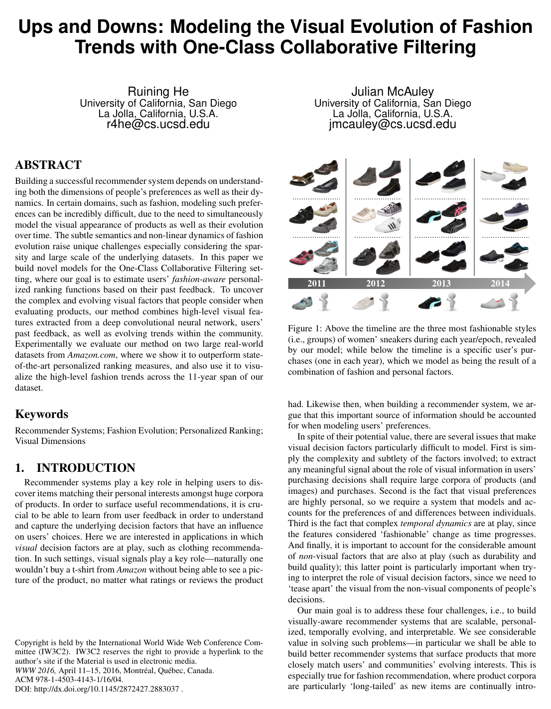
Building a successful recommender system depends on understanding both the dimensions of people's preferences as well as their dynamics. In certain domains, such as fashion, modeling such preferences can be incredibly difficult, due to the need to simultaneously model the visual appearance of products as well as their evolution over time. The subtle semantics and non-linear dynamics of fashion evolution raise unique challenges especially considering the sparsity and large scale of the underlying datasets. In this paper we build novel models for the One-Class Collaborative Filtering setting, where our goal is to estimate users' fashion-aware personalized ranking functions based on their past feedback. To uncover the complex and evolving visual factors that people consider when evaluating products, our method combines high-level visual features extracted from a deep convolutional neural network, users' past feedback, as well as evolving trends within the community. Experimentally we evaluate our method on two large real-world datasets from this http URL, where we show it to outperform state-of-the-art personalized ranking measures, and also use it to visualize the high-level fashion trends across the 11-year span of our dataset.

Topics

collaborative filtering convolutional neural networks http semantics visual feature recommendation user preferences personalized recommendation recommendation algorithms

Keywords

one-class collaborative filtering visual evolution fashion trends fashion dynamics Bayesian personalized ranking concept drift implicit feedback datasets matrix factorization temporal visual bias

1 Introduction
2 Modeling the Temporal Dynamics of Visual Styles
2.1 Matrix Factorization
2.2 Modeling Visual Dimensions
2.3 Modeling Visual Evolution
2.3.1 Temporally-evolving Visual Factors
2.3.2 Temporally-evolving Visual Bias
2.3.3 Non-Visual Temporal Dynamics
2.3.4 Fashion Epoch Segmentation
3 Learning the Model
3.1 Log-Likelihood Maximization
3.2 Coordinate Ascent Fitting Procedure
3.2.1 Fitting the Model Parameters Θ\Theta
3.2.2 Fitting the Fashion Epoch Segmentation Λ\Lambda
4 Experiments
4.1 Datasets
4.2 Visual Features
4.3 Evaluation Methodology
4.4 Comparison Methods
4.5 Performance
4.5.1 All Items & Cold Start
4.5.2 Results & Analysis
4.5.3 Reproducibility
4.6 Visualization
4.6.1 Visual Dimensions
4.6.2 Shifts in Fashion
4.7 Case Study: Men’s Fashion in the 2000s
5 Related Work
6 Conclusion
A Scalability Analysis
References

Knowls

Knowl 1 — Fashion-Aware Preference Predictor (TVBPR+)
model/method
In visually-aware recommendation with implicit feedback over time, the predicted affinity score $\hat{x}_{u,i}(t)$ of user $u \in \mathcal{U}$ toward item $i \in \mathcal{I}$ at timestamp $t$ is formulated to combine visual and non-visual user-item interactions alongside both visual and non-visual temporal dynamics:

$\hat{x}_{u,i}(t) = \alpha + \beta_u + \beta_i(t) + \beta_{C_i}(t) + \langle \beta(t), f_i \rangle + \langle \gamma_u, \gamma_i \rangle + \langle \theta_u(t), \theta_i(t) \rangle$

where:
- $\alpha \in \mathbb{R}$ is the global bias offset,
- $\beta_u \in \mathbb{R}$ is the stationary bias of user $u$ ,
- $\beta_i(t) \in \mathbb{R}$ is the time-dependent item bias of item $i$ , capturing item-level non-visual temporal variations (such as promotions or lifecycle effects),
- $\beta_{C_i}(t) \in \mathbb{R}$ is the time-dependent subcategory bias for the category $C_i$ containing item $i$ , capturing macro trends across product types,
- $f_i \in \mathbb{R}^F$ is an $F$ -dimensional visual feature vector extracted from an image of item $i$ via a deep convolutional neural network,
- $\beta(t) \in \mathbb{R}^F$ is a time-dependent visual bias vector capturing community-wide visual preferences at time $t$ ,
- $\gamma_u, \gamma_i \in \mathbb{R}^K$ are $K$ -dimensional latent factor vectors for user $u$ and item $i$ capturing non-visual preferences,
- $\theta_u(t) \in \mathbb{R}^{K'}$ is the $K'$ -dimensional visual preference vector of user $u$ at time $t$ (which can be kept stationary as $\theta_u$ when per-user interaction spans are short),
- $\theta_i(t) \in \mathbb{R}^{K'}$ is the $K'$ -dimensional time-dependent visual factor vector of item $i$ at time $t$ .
When evaluating personalized rankings for a single user $u$ , the user-independent offset $\alpha$ and user bias $\beta_u$ can be omitted.
Knowl 2 — Temporally-Evolving Item Visual Factors
equation
To model evolving fashion dynamics across an entire community while maintaining parameter efficiency, the visual factor vector $\theta_i(t) \in \mathbb{R}^{K'}$ of an item $i$ with visual feature vector $f_i \in \mathbb{R}^F$ at time $t$ is defined as:

$\theta_i(t) = (E f_i) \odot w(t) + \Delta E(t) f_i$

where:
- $E \in \mathbb{R}^{K' \times F}$ is a stationary visual embedding matrix mapping high-dimensional visual features $f_i$ to a lower-dimensional $K'$ -dimensional visual style space,
- $w(t) \in \mathbb{R}^{K'}$ is a time-dependent dimension-weighting vector modeling temporal weighting drift (shifting community emphasis on specific visual dimensions),
- $\odot$ denotes the element-wise Hadamard product,
- $\Delta E(t) \in \mathbb{R}^{K' \times F}$ is a time-dependent deviation embedding matrix modeling temporal attractiveness drift (gradual shifts in how visual features map to visual dimensions).
This formulation allows regularized low-rank structures to capture the base visual dimensions, the temporal dimension-weighting changes, and remaining temporal deviations.
Knowl 3 — Temporally-Evolving Visual Bias
equation
To capture common shifts in overall community responsiveness toward visual appearances independently of personalized interactions, the time-dependent visual bias vector $\beta(t) \in \mathbb{R}^F$ applied to item visual features $f_i \in \mathbb{R}^F$ is defined as:

$\beta(t) = \beta \odot b(t) + \Delta \beta(t)$

where:
- $\beta \in \mathbb{R}^F$ is a stationary base visual bias vector,
- $b(t) \in \mathbb{R}^F$ is a time-dependent weighting vector,
- $\odot$ is the Hadamard product,
- $\Delta \beta(t) \in \mathbb{R}^F$ is a time-dependent bias deviation vector.
The resulting visual bias contribution $\langle \beta(t), f_i \rangle$ explains general temporal shifts in product image attractiveness, leaving user-specific and dimension-specific variances to the higher-rank interaction terms.
Knowl 4 — Discrete Fashion Epoch Segmentation
model/method
Because real-world fashion evolution exhibits non-linear and abrupt shifts across time that standard continuous parametric time-decay functions cannot accurately capture, the dataset timeline is segmented into a partition $\Lambda$ consisting of $N$ contiguous discrete fashion epochs: $\Lambda = \{ep_1, ep_2, \dots, ep_N\}$ .

Each epoch $ep$ has an associated set of discretized temporal parameters:

$\Theta_{ep} = \{\Delta E(ep), \Delta \beta(ep), w(ep), b(ep), \beta_i(ep), \beta_{C_i}(ep)\}$

A segmentation function $ep(t)$ maps any continuous timestamp $t$ to its epoch index. The full parameter set to estimate comprises:

$\Theta = \bigcup_{ep=1}^N \Theta_{ep} \cup \{\alpha, \beta_u, \gamma_u, \gamma_i, \theta_u, E, \beta\}$

along with the partition boundaries $\Lambda$ .
Knowl 5 — Time-Aware Bayesian Personalized Ranking Objective
equation
Let $\mathcal{U}$ be the set of users, $\mathcal{I}$ the set of items, and $\mathcal{P}_u \subset \mathcal{I}^+_u$ the set of training items for which user $u$ expressed positive feedback at timestamp $t_{ui}$ . The training corpus of quadruples is defined as:

$\mathcal{D}_{S+} = \{(u, i, j, t_{ui}) \mid u \in \mathcal{U} \wedge i \in \mathcal{P}_u \wedge j \in \mathcal{I} \setminus \mathcal{P}_u\}$

Model parameters $\Theta$ and timeline segmentation $\Lambda$ are estimated by maximizing the regularized pairwise log-likelihood:

$\hat{\Theta}, \hat{\Lambda} = \arg\max_{\Theta, \Lambda} \sum_{(u, i, j, t_{ui}) \in \mathcal{D}_{S+}} \ln \sigma\left(\hat{x}_{u,i,j}(ep(t_{ui}))\right) - \frac{\lambda_\Theta}{2} \|\Theta\|_2^2$

where:
- $\sigma(z) = \frac{1}{1 + e^{-z}}$ is the logistic sigmoid function,
- $\hat{x}_{u,i,j}(ep(t_{ui})) = \hat{x}_{u,i}(ep(t_{ui})) - \hat{x}_{u,j}(ep(t_{ui}))$ is the predicted difference in preference between observed item $i$ and unobserved item $j$ evaluated at epoch $ep(t_{ui})$ ,
- $\lambda_\Theta \ge 0$ is the $L_2$ regularization hyperparameter.
Knowl 6 — Coordinate Ascent Fitting Procedure for TVBPR+
algorithm
Joint optimization of model parameters $\Theta$ and epoch partition $\Lambda$ is performed via coordinate ascent, alternating between stochastic gradient ascent on $\Theta$ and dynamic programming on $\Lambda$ .
Input: Training quadruples $\mathcal{D}_{S+}$ , learning rate $\epsilon$ , regularization parameter $\lambda_\Theta$ , number of epochs $N$ , timeline partitioned into candidate bins
Output: Model parameters $\Theta$ and epoch segmentation $\Lambda$
Initialize parameters $\Theta$ randomly in $[0, 1.0]$
Initialize $\Lambda$ as $N$ equal-sized continuous segments
repeat
    // Step 1: Parameter Optimization (Fixed epoch segmentation $\Lambda$ )
    for iteration = 1 to 100 do
        for each sampled quadruple $(u, i, j, t_{ui}) \in \mathcal{D}_{S+}$ do
             $ep \leftarrow ep(t_{ui})$
             $\hat{x}_{uij} \leftarrow \hat{x}_{u,i}(ep) - \hat{x}_{u,j}(ep)$
             $\Theta \leftarrow \Theta + \epsilon \cdot \left(\sigma(-\hat{x}_{uij}) \frac{\partial \hat{x}_{uij}}{\partial \Theta} - \lambda_\Theta \Theta\right)$
        end for
    end for
    // Step 2: Epoch Segmentation Optimization (Fixed parameters $\Theta$ )
    Compute corpus log-likelihood across candidate temporal bins by approximating with a sampled batch of negative items
     $\Lambda \leftarrow \text{DynamicProgramming}(\text{bin likelihoods}, N)$
until convergence on validation set
return $\Theta, \Lambda$
The sequence segmentation dynamic program takes $O(|\mathcal{D}_{S+}| \times N)$ time. Parameter updates take $O(K + K')$ per sampled quadruple since only the active epoch's parameters are updated.
Knowl 7 — Item Visual Score and Normalized Visual Score
definition
The overall community visual popularity of an item $i$ at epoch $ep$ , termed its Visual Score, is defined by averaging the visual components of the preference predictor across all users $\mathcal{U}$ :

$\text{VisualScore}(i, ep) = \frac{1}{|\mathcal{U}|} \sum_{u \in \mathcal{U}} \langle \theta_u, \theta_i(ep) \rangle + \langle \beta(ep), f_i \rangle$

where $\theta_u \in \mathbb{R}^{K'}$ is the visual factor of user $u$ , $\theta_i(ep) \in \mathbb{R}^{K'}$ is the item visual factor at epoch $ep$ , $\beta(ep) \in \mathbb{R}^F$ is the visual bias vector at epoch $ep$ , and $f_i \in \mathbb{R}^F$ is the deep CNN feature vector of item $i$ .

To observe visual popularity shifts across time independently of overall volume changes, the Normalized Visual Score is computed by subtracting the average visual score of all items in epoch $ep$ :

$\text{NormalizedVisualScore}(i, ep) = \text{VisualScore}(i, ep) - \frac{1}{|\mathcal{I}|} \sum_{j \in \mathcal{I}} \text{VisualScore}(j, ep)$
Knowl 8 — Experimental Setup and Evaluation Protocol for Temporal Fashion Recommendation
experimental setup
The experimental evaluation is conducted on two Amazon.com implicit feedback datasets spanning March 2003 to July 2014:
- Women's Clothing & Accessories: 99,748 users, 331,173 items, 854,211 positive interactions.
- Men's Clothing & Accessories: 34,212 users, 100,654 items, 260,352 positive interactions.
Users with fewer than 5 interactions are filtered out. For each user $u$ , two interactions are held out uniformly at random: one for validation $V_u$ and one for testing $T_u$ , leaving the remaining items $\mathcal{P}_u$ for training ( $|\mathcal{P}_u| = |V_u| = |T_u| = |\mathcal{U}|$ ). Visual features ( $F=4096$ ) are extracted from the second fully connected layer (FC7) of a pre-trained Caffe AlexNet CNN (pre-trained on 1.2 million ImageNet ILSVRC2010 images).

Evaluation is performed on test interactions $\mathcal{T} = \bigcup_{u \in \mathcal{U}} T_u$ using Area Under the ROC Curve (AUC):

$\text{AUC} = \frac{1}{|\mathcal{U}|} \sum_{u \in \mathcal{U}} \frac{1}{|E(u)|} \sum_{(i,j) \in E(u)} \delta\left(\hat{x}_{u,i}(t_{ui}) > \hat{x}_{u,j}(t_{ui})\right)$

where $E(u) = \{(i, j) \mid i \in T_u \wedge j \notin (\mathcal{P}_u \cup V_u \cup T_u)\}$ and $\delta(\cdot)$ is the indicator function.

Two test settings are reported:
- All Items: Evaluates the average AUC across all test items in $\mathcal{T}$ .
- Cold Start: Evaluates AUC strictly on test items that had fewer than 5 positive feedback instances in the training set (accounting for approximately 60% of test items).
All matrix factorization models use a total dimension of 20 (split evenly as $K=10$ non-visual and $K'=10$ visual dimensions for visually-aware models). Regularization hyperparameter $\lambda_\Theta = 1$ is used for BPR models, with $\Delta E(t), w(t), b(t)$ regularized at $0.0001$ .

Knowl 9 — Personalized Ranking Performance on Amazon Fashion Datasets

data/table

The test AUC performance across All Items and Cold Start evaluation settings on Amazon Women's and Men's Clothing & Accessories (total dimensions = 20; 10 epochs for temporal models, with 5 epochs reported for TVBPR+(5)):

Dataset	Setting	POP	WR-MF	BPR-MF	BPR-TMF	VBPR	TVBPR	TVBPR+(5)	TVBPR+(10)
Women	All Items	0.5726	0.6441	0.7020	0.7259	0.7834	0.8117	0.8148	0.8210
	Cold Start	0.3214	0.5195	0.5281	0.5749	0.6813	0.7325	0.7355	0.7469
Men	All Items	0.5772	0.6228	0.7100	0.7069	0.7841	0.8064	0.8074	0.8084
	Cold Start	0.3159	0.5124	0.5512	0.5498	0.6898	0.7314	0.7373	0.7459

Key results:

Visual features provide large gains over non-visual models: static VBPR improves AUC over non-visual BPR-MF by 11.6% (Women) and 10.4% (Men) on All Items, and by 29.0% (Women) and 25.1% (Men) on Cold Start items.
Visual temporal dynamics provide significant further gains: TVBPR improves over static VBPR by 3.6% (Women) and 2.8% (Men) on All Items, and by 7.5% (Women) and 6.0% (Men) on Cold Start.
TVBPR+ (combining visual and non-visual temporal dynamics with 10 epochs) achieves the best performance, outperforming static VBPR by 4.8% on All Items and 9.6% on Cold Start for Women, and 3.1% on All Items and 8.1% on Cold Start for Men.
Non-visual temporal modeling alone (BPR-TMF) produces much smaller gains over BPR-MF (1.5% for All Items, 4.3% for Cold Start on average) compared to modeling visual temporal evolution.

Knowl 10 — Non-Linearity of Visual Dimension Evolution and Men's Fashion Resurgence
empirical result
Visualizing the learned dimension weights $w_k(t)$ and normalized visual scores across epochs reveals distinct behavioral patterns in fashion evolution:
1. Dimension weights $w_k(t)$ for discovered visual styles (such as semi-formal vs. casual clothing, graphic prints, and specific texture/color patterns) evolve non-linearly across the 2004–2014 period, demonstrating why continuous linear or monotonic parametric temporal decay functions underperform discrete epoch segmentation.
2. In a case study on Men's Clothing using historical late-2000s resurgence trends as ground truth, query items representing 1950s/1980s resurgence styles (Ed Hardy t-shirts, Hawaiian shirts, black leather jackets, and ski jackets) showed sharp increases in Normalized Visual Score specifically beginning in 2009 in the model's learned visual space.
3. Visual signals are shown to be essential for handling cold-start items, which make up roughly 60% of test instances in clothing recommendation.

Coverage note — The parametric user temporal drift formula $\theta_u(t) = \theta_u + \text{sign}(t - t_u)|t - t_u|^\kappa \eta_u$ was omitted as a separate model knowl because the paper explicitly discarded it in favor of stationary user factors due to user sparsity and short active lifespans.

References

1.D. W. Aha, D. Kibler, and M. K. Albert. Instance-based learning algorithms. Machine learning, 1991.
2.R. M. Bell, Y. Koren, and C. Volinsky. The bellkor solution to the netflix prize, 2007.
3.R. Bellman. On the approximation of curves by line segments using dynamic programming. Communications of the ACM, 1961.
4.J. Bennett and S. Lanning. The netflix prize. In KDDCup, 2007.
5.T. Cebrián, M. Planagumà, P. Villegas, and X. Amatriain. Music recommendations with temporal context awareness. In RecSys, 2010.
6.W. Di, N. Sundaresan, R. Piramuthu, and A. Bhardwaj. Is a picture really worth a thousand words?-on the role of images in e-commerce. In WSDM, 2014.
7.Y. Ding and X. Li. Time weight collaborative filtering. In CIKM, 2005.
8.J. Donahue, Y. Jia, O. Vinyals, J. Hoffman, N. Zhang, E. Tzeng, and T. Darrell. Decaf: A deep convolutional activation feature for generic visual recognition. In ICML, 2014.
9.Z. Gantner, S. Rendle, C. Freudenthaler, and L. Schmidt-Thieme. Mymedialite: A free recommender system library. In RecSys, 2011.
10.J. H. Gilkeson and K. Reynolds. Determinants of internet auction success and closing price: An exploratory study. Psychology & Marketing, 2003.
11.A. Goswami, N. Chittar, and C. H. Sung. A study on the impact of product images on user clicks for online shopping. In WWW, 2011.
12.R. He and J. McAuley. Vbpr: Visual bayesian personalized ranking from implicit feedback. CoRR, 2015.
13.Y. Hu, Y. Koren, and C. Volinsky. Collaborative filtering for implicit feedback datasets. In ICDM. IEEE, 2008.
14.V. Jagadeesh, R. Piramuthu, A. Bhardwaj, W. Di, and N. Sundaresan. Large scale visual recommendations from street fashion images. In SIGKDD, 2014.
15.Y. Jia, E. Shelhamer, J. Donahue, S. Karayev, J. Long, R. B. Girshick, S. Guadarrama, and T. Darrell. Caffe: Convolutional architecture for fast feature embedding. In MM, 2014.
16.Y. Kalantidis, L. Kennedy, and L.-J. Li. Getting the look: clothing recognition and segmentation for automatic product suggestions in everyday photos. In ICMR, 2013.
17.S. Karayev, M. Trentacoste, H. Han, A. Agarwala, T. Darrell, A. Hertzmann, and H. Winnemoeller. Recognizing image style. In BMVC, 2014.
18.R. Klinkenberg. Learning drifting concepts: Example selection vs. example weighting. Intelligent Data Analysis, 2004.
19.Y. Koren. Collaborative filtering with temporal dynamics. Communications of the ACM, 2010.
20.Y. Koren and R. Bell. Advances in collaborative filtering. In Recommender systems handbook. Springer, 2011.
21.A. Krizhevsky, I. Sutskever, and G. E. Hinton. Imagenet classification with deep convolutional neural networks. In NIPS, 2012.
22.A. Krohn-Grimberghe, L. Drumond, C. Freudenthaler, and L. Schmidt-Thieme. Multi-relational matrix factorization using bayesian personalized ranking for social network data. In WSDM, 2012.
23.N. Lathia, S. Hailes, L. Capra, and X. Amatriain. Temporal diversity in recommender systems. In SIGIR, 2010.
24.X. Lu, Z. Lin, H. Jin, J. Yang, and J. Z. Wang. RAPID: rating pictorial aesthetics using deep learning. In MM, 2014.
25.J. J. McAuley and J. Leskovec. From amateurs to connoisseurs: modeling the evolution of user expertise through online reviews. In WWW, 2013.
26.J. J. McAuley, C. Targett, Q. Shi, and A. van den Hengel. Image-based recommendations on styles and substitutes. In SIGIR, 2015.
27.R. Pan, Y. Zhou, B. Cao, N. N. Liu, R. Lukose, M. Scholz, and Q. Yang. One-class collaborative filtering. In ICDM, 2008.
28.W. Pan and L. Chen. Gbpr: Group preference based bayesian personalized ranking for one-class collaborative filtering. In IJCAI, 2013.
29.U. Paquet and N. Koenigstein. One-class collaborative filtering with random graphs. In WWW, 2013.
30.S. Rendle, C. Freudenthaler, Z. Gantner, and L. Schmidt-Thieme. Bpr: Bayesian personalized ranking from implicit feedback. In UAI, 2009.
31.O. Russakovsky, J. Deng, H. Su, J. Krause, S. Satheesh, S. Ma, Z. Huang, A. Karpathy, A. Khosla, M. S. Bernstein, A. C. Berg, and L. Fei-Fei. Imagenet large scale visual recognition challenge. CoRR, 2014.
32.E. Simo-Serra, S. Fidler, F. Moreno-Noguer, and R. Urtasun. Neuroaesthetics in fashion: Modeling the perception of fashionability. In CVPR, 2014.
33.D. H. Stern, R. Herbrich, and T. Graepel. Matchbox: large scale online bayesian recommendations. In WWW, 2009.
34.A. Tsymbal. The problem of concept drift: definitions and related work. Technical Report, 2004.
35.L. van der Maaten. Accelerating t-sne using tree-based algorithms. Journal of machine learning research, 2014.
36.A. Veit, B. Kovacs, S. Bell, J. McAuley, K. Bala, and S. Belongie. Learning visual clothing style with heterogeneous dyadic co-occurrences. In ICCV, 2015.
37.H. Wang, W. Fan, P. S. Yu, and J. Han. Mining concept-drifting data streams using ensemble classifiers. In SIGKDD, 2003.
38.X. Yi, L. Hong, E. Zhong, N. N. Liu, and S. Rajan. Beyond clicks: dwell time for personalization. In RecSys, 2014.
39.Y. Zhang, M. Zhang, Y. Zhang, G. Lai, Y. Liu, H. Zhang, and S. Ma. Daily-aware personalized recommendation based on feature-level time series analysis. In WWW, 2015.
40.T. Zhao, J. McAuley, and I. King. Leveraging social connections to improve personalized ranking for collaborative filtering. In CIKM, 2014.

Citation

MLA

He, R., and J. McAuley. “Ups and Downs”. Proceedings of the 25th International Conference on World Wide Web, 2016, pp. 507–17, https://doi.org/10.1145/2872427.2883037.

APA

He, R., & McAuley, J. (2016). Ups and Downs. Proceedings of the 25th International Conference on World Wide Web, 507–517. https://doi.org/10.1145/2872427.2883037

Chicago

He, R., and J. McAuley. 2016. “Ups and Downs”. Proceedings of the 25th International Conference on World Wide Web, 507–17. https://doi.org/10.1145/2872427.2883037.

Harvard

He, R. and McAuley, J. (2016) “Ups and Downs”, Proceedings of the 25th International Conference on World Wide Web. International World Wide Web Conferences Steering Committee, pp. 507–517. Available at: https://doi.org/10.1145/2872427.2883037.

Vancouver

1. He R, McAuley J (2016) Ups and Downs. In: Proceedings of the 25th International Conference on World Wide Web. International World Wide Web Conferences Steering Committee, pp 507–517

BibTeX

@inproceedings{He_2016, series={WWW ’16}, title={Ups and Downs: Modeling the Visual Evolution of Fashion Trends with One-Class Collaborative Filtering}, url={http://dx.doi.org/10.1145/2872427.2883037}, DOI={10.1145/2872427.2883037}, booktitle={Proceedings of the 25th International Conference on World Wide Web}, publisher={International World Wide Web Conferences Steering Committee}, author={He, Ruining and McAuley, Julian}, year={2016}, month=Apr, pages={507–517}, collection={WWW ’16} }

Metadata:Crossref

Source Code

This paper has an official code repository available. Click below to access the source code.

View Repository

Access the Paper

This paper is available from its original source. Click below to access the PDF.

Open PDF

Ups and Downs: Modeling the Visual Evolution of Fashion Trends with One-Class Collaborative Filtering

Abstract

Topics

Keywords

Table of Contents

Knowls

Knowl 1 — Fashion-Aware Preference Predictor (TVBPR+)

Knowl 2 — Temporally-Evolving Item Visual Factors

Knowl 3 — Temporally-Evolving Visual Bias

Knowl 4 — Discrete Fashion Epoch Segmentation

Knowl 5 — Time-Aware Bayesian Personalized Ranking Objective

Knowl 6 — Coordinate Ascent Fitting Procedure for TVBPR+

Knowl 7 — Item Visual Score and Normalized Visual Score