Always Learning, Always Mixing: Efficient and Simple Data Mixing All The Time

Michael Y. Hu$^{1}$ Apurva Gandhi$^{2}$
Kyunghyun Cho$^{1}$ Tal Linzen$^{1}$ Pratyusha Sharma$^{1,3}$
$^{1}$ New York University $^{2}$ Carnegie Mellon University $^{3}$ Microsoft
{michael.hu, kyunghyun.cho, linzen}@nyu.edu
[email protected] [email protected]

Abstract

Data mixing decides how to combine different sources or types of data and is a consequential problem throughout language model training. In pretraining, data composition is a key determinant of model quality; in continual learning and adaptation, it governs what is retained and acquired. Yet existing data mixing methods address only one phase of this lifecycle at a time: some require smaller proxy models tied to a single training phase, others assume a fixed domain set, and continual learning lacks principled guidance altogether. We argue that data mixing is fundamentally an online decision making problem—one that recurs throughout training and demands a single, unified solution. We introduce OP-MIX (On-Policy Mix), a data mixing algorithm that operates across the entire language model training lifecycle. Our main insight is that candidate data mixtures can be cheaply simulated by interpolating between low-rank adapters trained directly on the current model, eliminating separate proxy models and ensuring the search is always grounded in the model's actual learning dynamics. Across pretraining, continual midtraining, and continual instruction tuning, OP-MIX consistently finds near-optimal mixtures while using a fraction of the compute of the baselines. In pretraining, OP-MIX improves upon training without mixing by 6.3% in average perplexity. For continual learning, OP-MIX matches the performance of both retraining and on-policy distillation while using 66% and 95% less overall compute, respectively. OP-MIX suggests a different view of language model training: not a sequence of distinct phases, but a single continuous process of learning from data.

Preprint. Code: https://github.com/michahu/on-policy-mix

Executive Summary: Language model training requires repeated decisions about how to combine data from different sources or domains. These choices strongly affect final model quality during pretraining, how well a model incorporates new information without losing prior knowledge during midtraining, and its performance on instruction-following tasks. Existing methods for selecting data proportions, however, tend to target only one phase, rely on separate small proxy models, or assume a fixed set of data sources. As new datasets arrive over time, these constraints make it difficult to maintain efficient, principled mixing across the full training process.

The paper introduces OP-MIX, a single algorithm designed to find good data mixtures at any stage of language model development. It trains one low-rank adapter (LoRA) per domain directly on the current model, then uses linear interpolation between those adapters to simulate many possible mixture ratios without additional full training runs. The method fits a simple regression to the resulting loss surface, selects an optimal balance between old and new data, and expands the mixture when fresh domains appear. The authors tested it on models from 150 million to 7 billion parameters across pretraining on five domains, successive midtraining updates, and continual instruction tuning on tool-use, science, and medical tasks.

OP-MIX improves average perplexity by 6.3 percent over training without any mixing and matches the strongest baseline while using 14 percent less compute in pretraining. In continual midtraining it nearly equals the performance of full retraining from scratch while cutting compute by up to 66 percent and reduces forgetting by 27 percent on average relative to standard continual fine-tuning. In instruction tuning it recovers the gains of a more expensive self-distillation method with 95 percent less compute and combines with that method for further improvement. The approach consistently lies on the performance-efficiency frontier in all three settings.

These results show that data mixing can be treated as one ongoing process rather than a series of separate problems. The efficiency gains make it practical to re-optimize mixtures whenever new data arrives, lowering both overall training cost and the risk of catastrophic forgetting. The findings also indicate that data proportion choices and training-objective modifications act as largely independent levers for continual learning.

Practitioners should consider adopting OP-MIX or similar on-policy mixing strategies for new model training runs, especially in settings where data domains continue to evolve. Teams may also benefit from first running a short pilot on a subset of domains to confirm the approximation remains accurate at their scale. Further work is needed to verify behavior on models above 70 billion parameters and with ten or more domains before very large deployments. The reported gains rest on experiments up to 530 million parameters for pretraining and midtraining and 7 billion for instruction tuning; extrapolation beyond these regimes should be treated with caution until larger-scale confirmation is available.

1. Introduction

Section Summary: Language models are typically trained on mixtures of data from various sources, but determining the ideal proportions is difficult and becomes even harder when new data domains continually appear, as existing methods require expensive retraining of many smaller models and struggle to adapt without forgetting prior knowledge. The proposed OP-Mix approach addresses this by training a single low-rank adapter for each domain directly from the current model and using simple linear combinations of those adapters to estimate performance for any mixture ratio, avoiding the need to retrain proxies repeatedly. Evaluations show that this method works effectively across pretraining, midtraining, and instruction tuning stages, delivering strong results with far less computation while naturally incorporating new data.

Language models are trained on carefully curated data mixtures, yet the science of constructing the right mixture remains nascent. The dominant approach—training small proxy models on candidate mixtures and extrapolating to full training—is combinatorially expensive and scales poorly as the number of domains grows ([1, 2, 3]). Furthermore, most data mixing approaches are specialized towards pretraining and assume a fixed domain set ([4, 5, 6, 7, 8]): in practice, available training domains evolve continuously as new tasks are defined, new corpora are collected, and new capabilities are prioritized. This induces a natural continual learning problem, where the goal is to incorporate new data without catastrophically forgetting what the model has already learned. We ask:

What is the right data mix, and how do we find it efficiently as the data itself keeps changing?

We propose $\textsc{OP-Mix}$ (On-Policy Mix), an algorithm that estimates optimal data mixtures by combining two insights. First, rather than train separate proxy models for each candidate data mixture, $\textsc{OP-Mix}$ trains a single low-rank adapter (LoRA, [9]) per data domain directly from the current model, keeping the proxy model on-policy with the model being trained—i.e. reflective of its current state. Second, it uses linear interpolation between LoRAs as a proxy for the loss surface of full data mixing, following recent works ([10, 11]). This bypasses the need to retrain proxies for every different data mix ratio, escaping the combinatorial explosion of training runs. These two insights allow $\textsc{OP-Mix}$ to search over data mixtures with minimal additional compute, no separate proxy models, and natural accommodation to new domains: when a new dataset arrives, we simply train another LoRA and re-fit the mixture.

We evaluate $\textsc{OP-Mix}$ across three stages of the language model lifecycle—pretraining ([12, 13]), continual midtraining ([14, 15]), and continual instruction tuning ([16])—and find that our single algorithm suffices for all three. In pretraining, $\textsc{OP-Mix}$ improves over no data mixing by 6.3% in average perplexity and matches the best data mixing baseline's performance while using 14% less compute. In continual midtraining, $\textsc{OP-Mix}$ achieves the performance of full retraining at a fraction of the cost. Finally, in continual instruction tuning, $\textsc{OP-Mix}$ composes with on-policy self-distillation ([17, 18, 19]), yielding further gains without modifications to either algorithm. Our contributions are as follows:

1. The first universal data mixing algorithm:$\textsc{OP-Mix}$ is the first data mixing algorithm that both expands to new data domains and simulates candidate mixtures without separate proxy models. This enables $\textsc{OP-Mix}$ to continually mix data even as the data evolves, overcoming the need for a different algorithm at each phase of the training pipeline (§ 3).
2. State-of-the-art across the entire training lifecycle: A single instantiation of $\textsc{OP-Mix}$ achieves state-of-the-art performance in pretraining, continual midtraining, and continual instruction tuning, demonstrating that phase-specific algorithms are unnecessary. (§ 4).
3. $\textsc{OP-Mix}$ enables continual learning, matching on-policy distillation with 95% less compute: Applied atop standard SFT during continual instruction tuning, $\textsc{OP-Mix}$ recovers the gains of self-distillation finetuning (SDFT, [17]) at a fraction of the cost. Combining $\textsc{OP-Mix}$ with SDFT also yields further gains, suggesting that data mixing can be an independent axis of improvement from training objective (§ 4.1).

2. Background: Data Mixing and Its Limitations

Section Summary: Data mixing involves choosing proportions of training data from multiple sources, or domains, in order to improve a language model's performance on downstream tasks while minimizing a combined loss. Algorithms typically predict future results with simple scaling laws fitted on smaller, cheaper proxy models run with different mixtures, then select the best proportions for the full training run. Existing approaches have key drawbacks: most cannot incorporate new datasets that arrive midway through training, and reliance on separate proxies makes them impractical or inaccurate after pretraining, leaving a gap for methods that work seamlessly across the entire model lifecycle.

Let $\mathcal{D} = {D_1, D_2, \dots, D_m}$ be a set of $m$ data domains, where domain $D_i$ has $N_i$ tokens. A data mixture is a probability vector $p \in \triangle^{m-1}$, where training on $R$ total tokens uses $p_i \cdot R$ tokens from domain $D_i$. We denote a language model of $S$ parameters trained for $R$ tokens on mixture $p$ as $\text{LM}(S, R, p)$ and measure its performance on downstream task $j \in [J]$ as $f_j(\text{LM}(S, R, p))$. We assume the training objective is to minimize a weighted sum $F = \sum_j w_j \cdot f_j(\text{LM}(S, R, p))$, where weights $w_j$ are user-specified. Here, metrics intended to be maximized (e.g. accuracy) are negated.

Batch continual learning.

During training, we may periodically receive $k$ new datasets $D_{m+1}, \dots, D_{m+k}$, in which case the updated domain set becomes $\mathcal{D} \cup {D_{m+1}, \dots, D_{m+k}}$. For example, these $k$ new datasets may be instruction fine-tuning datasets, introduced after pretraining. We may then aim to minimize the loss across both pretraining and instruction tuning datasets.

Data mixing.

Data mixing algorithms automate the process of finding the mixture $p$ that minimizes $F$. The core idea in most data mixing algorithms is fitting a simple model $\hat{f_i}(p)$ that predicts the future performance $f_i$ as a function of the performance on the current data mixture $p$ (see [4] for review). One can then minimize $\hat{f_i}(p)$ to estimate an optimal mixture.

\begin{tabular}{@l l p{1.55cm} p{1.3cm}@}
\toprule
\multicolumn{2}{@l}{Algorithm} & Adapts to new data? & No proxy models? \\
\midrule
ADO & ([6]) & \textcolor{red}{\ding{55}} & \arraybackslash \textcolor{green!70!black}{\ding{51}} \\
Aioli & ([4]) & \textcolor{red}{\ding{55}} & \arraybackslash \textcolor{red}{\ding{55}} \\
DoGE & ([5]) & \textcolor{red}{\ding{55}} & \arraybackslash \textcolor{green!70!black}{\ding{51}} \\
GRAPE & ([20]) & \textcolor{red}{\ding{55}} & \arraybackslash \textcolor{green!70!black}{\ding{51}} \\
OLMix & ([3]) & \textcolor{green!70!black}{\ding{51}} & \arraybackslash \textcolor{red}{\ding{55}} \\
RegMix & ([2]) & \textcolor{red}{\ding{55}} & \arraybackslash \textcolor{red}{\ding{55}} \\
MergeMix & ([10]) & \textcolor{red}{\ding{55}} & \arraybackslash \textcolor{green!70!black}{\ding{51}} \\
\midrule
\textsc{OP-Mix} & (ours) & \textcolor{green!70!black}{\ding{51}} & \arraybackslash \textcolor{green!70!black}{\ding{51}} \\
\bottomrule
\end{tabular}

Previous work has shown that future performance is well-predicted by a log-linear parametric form: $\hat{f_i}(p) = c_i + \exp{(A_i^\top p_i)}$, where $c_i \in \mathbb{R}$ and $A_i \in \mathbb{R}^m$ ([1, 4, 3]). Data mixing algorithms then aim to estimate such a scaling law as cheaply as possible. A common technique is to fit the scaling law by randomly sampling mixtures from the probability simplex and training proxy models with fewer parameters $S' \ll S$ and less data $R' \ll R$ to approximate the full model's performance on a data mixture: $f_i(\text{LM}(S, R, p)) \approx f_i(\text{LM}(S', R', p))$ ([2, 3, 1]).

A single data mixing algorithm that spans all of LM training is desirable for both practical reasons (less complexity and phase-specific tuning) and conceptual ones: pretraining, midtraining, and finetuning are not fundamentally different problems for data mixing. However, two issues limit existing algorithms from operating across this lifecycle. First, most data mixing algorithms, being targeted towards pretraining, do not expand their data mixtures. It follows that these algorithms cannot be applied to the continual learning setting, and yet language model training induces a natural continual learning problem from phase to phase. Second, data mixing methods that rely on separate proxy models are defunct after pretraining, as open-source model releases typically do not come with a matching small-model proxy ([21, 22, 23]). Moreover, separate smaller proxy models have been shown to yield suboptimal mixtures for the target model, as they diverge from the base model's dynamics at scale ([6, 3]) and the number of proxies explodes combinatorially with the number of datasets.

3. $\textsc{OP-Mix}$: On-Policy Data Mixing

Section Summary: OP-Mix is a practical method for automatically choosing good data mixtures throughout language model training, whether during initial pretraining or later stages when new data sources appear. Instead of training a separate model to test each possible mix, it attaches lightweight LoRA adapters to the actual model being trained, then combines those adapters in different proportions to simulate how various mixtures would perform. This lets the approach cheaply evaluate many blend ratios with only forward passes, fit a simple surface to the results, and pick the mixture that minimizes estimated loss before running the full training step.

In this work, we propose $\textsc{OP-Mix}$, a data mixing algorithm that works effectively for any stage of language model training by using on-policy proxies instead of separate proxies and efficiently expanding data mixtures. On-policy here means that the proxy is built from the model being trained, rather than a separately initialized model whose learning dynamics may diverge from its target. $\textsc{OP-Mix}$ uses Low-Rank Adaptation (LoRA, [9]) to cheaply estimate the performance of full training. LoRA reduces the necessary compute for testing new data mixtures while being tied to the base model and circumvents the ambiguities of creating separate proxy models later in training.

To simulate new data mixtures without performing additional training runs, we interpolate LoRA weights, as inspired by [10] and [11]. This allows us to train one LoRA per data domain and estimate the effect of mixing domains post-hoc using only forward passes. We also expand the data mixture when new domains arrive, taking inspiration from pretraining mixture reuse in [3]. In each stage, instead of retraining a new LoRA for every previously seen domain, we train a single "old" adapter $\theta_{D_{\text{old}}}^{\text{LoRA}}$, keeping probabilities of old domains constant and only adjusting the ratio between the old mixture and incoming new domains.

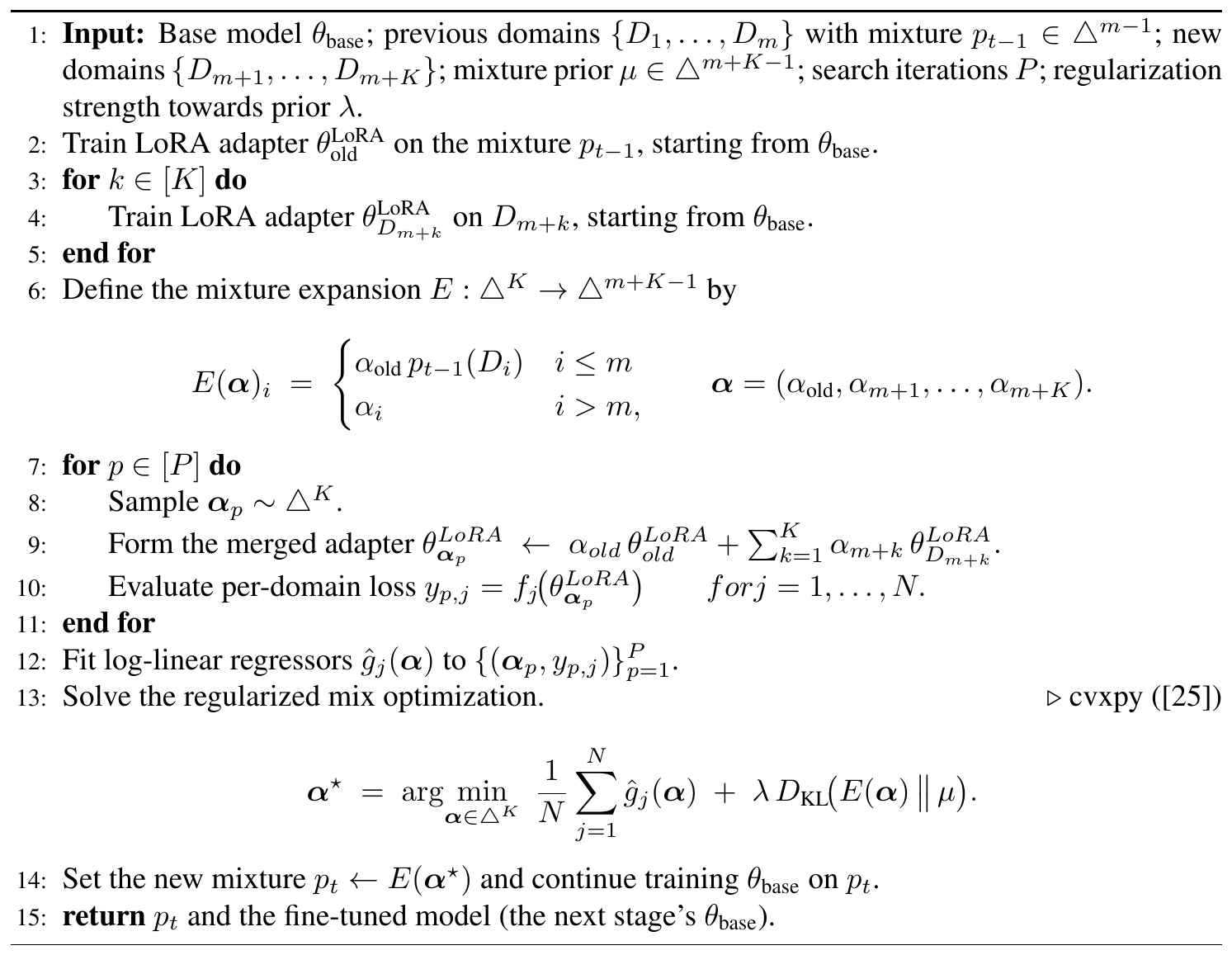
$\textsc{OP-Mix}$ (Algorithm 1).

In the continual setting, when $K$ new domains $D_{m+i}, i \in [K]$ arrive, we train a single LoRA adapter per domain $D_{m+i}$, starting from the current model. This gives us $\theta_{D_{m+i}}^{\text{LoRA}}$, a cheap approximation of what full finetuning on $D_{m+i}$ would produce. We also train $\theta_{D_{\text{old}}}^{\text{LoRA}}$ on the old data to approximate continued training on $D_{\text{old}}$. Next, we evaluate linear interpolation merges of $\theta_{D_{m+1}}^{\text{LoRA}}, \dots, \theta_{D_{m+K}}^{\text{LoRA}}$ and $\theta_{D_{\text{old}}}^{\text{LoRA}}$. We sample interpolation points in the $K$-simplex $\triangle^{K}$, and each interpolation point simulates a different mixing ratio between old and new data without additional training. We then fit a regression model to these evaluations, producing a smooth loss surface over the interpolation path (Algorithm 1, lines 7–12). Finally, we minimize over this surface to obtain $\alpha^\star$, the tradeoff between old and new data, distribute the resulting weight across all datasets, and do the final training run. See Figure 1 for a visual overview.

For pretraining, we begin with a warmup phase in which every document is sampled with equal probability (empirical risk minimization). After warmup, we reintroduce each dataset as new domains to adjust the data mixture. In § 4.1, we set warmup to 20% of the overall token budget.

4. Experimental Results

Section Summary: In experiments spanning pretraining, continual midtraining, and continual instruction tuning, OP-Mix adaptively optimizes data mixtures and delivers strong results across model sizes from 150M to 530M parameters. It matches or beats established baselines such as ERM, MergeMix, and OLMix in pretraining while using up to 14 percent less compute, and it substantially reduces catastrophic forgetting in continual settings, often approaching the performance of full retraining with roughly two-thirds less compute. These gains hold whether the objective is standard cross-entropy loss or on-policy distillation, confirming the method’s broad usefulness throughout the language-model lifecycle.

We examine $\textsc{OP-Mix}$ in several settings: pretraining, continual midtraining, and continual instruction fine-tuning. In pretraining, we examine $\textsc{OP-Mix}$ 's ability to find a good pretraining mixture for fixed training corpora. In midtraining ([14]), high quality datasets are upweighted relative to the original pretraining data mixture; here we continually finetune a pretrained model ladder from HuggingFace on successive reference datasets. Finally, we apply $\textsc{OP-Mix}$ to the continual instruction tuning setting, where a language model is finetuned on successive question-answering datasets, and consider two different objectives: cross-entropy loss and on-policy distillation ([17, 18, 19]). Further training details and hyperparameter choices are in Appendix A.

Pretraining baselines.

ERM samples from each data domain with probability proportional to domain size, equivalent to not optimizing the data mixture. MergeMix ([10]) finetunes independent models on each dataset, merges to simulate mixing, and uses regression to estimate the optimal mixture; we adapt it to pretraining with a 20% ERM warmup before finetuning (see Appendix A.2 for more details). It is a natural comparison—essentially $\textsc{OP-Mix}$ without data mixture expansion (Algorithm 1, line 6) and with full finetuning in place of LoRA. OLMix ([3]) trains small proxy models on randomly sampled mixtures over datasets and uses regression to estimate the optimal mixture.

Continual learning baselines.

Continual fine-tuning with WSD-S ([24]) trains on each dataset in succession with no replay of old data, using Weight-Stable-Decay-Simplified, a learning rate schedule designed for continual learning. For simplicity, we use WSD-S for all methods, including $\textsc{OP-Mix}$. 10% data replay extends the observation of [26] that having 10% of finetuning data be pretraining data mitigates catastrophic forgetting; we train with a 1:9 ratio between old and new data. Retraining (skyline): After training for $K \cdot R$ tokens from $K$ datasets and receiving a $(K{+}1)$ th dataset, train again for $(K{+}1) \cdot R$ tokens over all $K{+}1$ datasets.

To our knowledge, there currently are no adaptive data mixing baselines for continual learning. As noted in § 2, existing data mixing methods either operate over fixed data domains or require separate proxy models initialized from scratch.

4.1 $\textsc{OP-Mix}$ Works Across the Language Model Lifecycle

Across pretraining, continual midtraining, and continual instruction tuning, $\textsc{OP-Mix}$ achieves state-of-the-art performance (Figure 4–Figure 6).

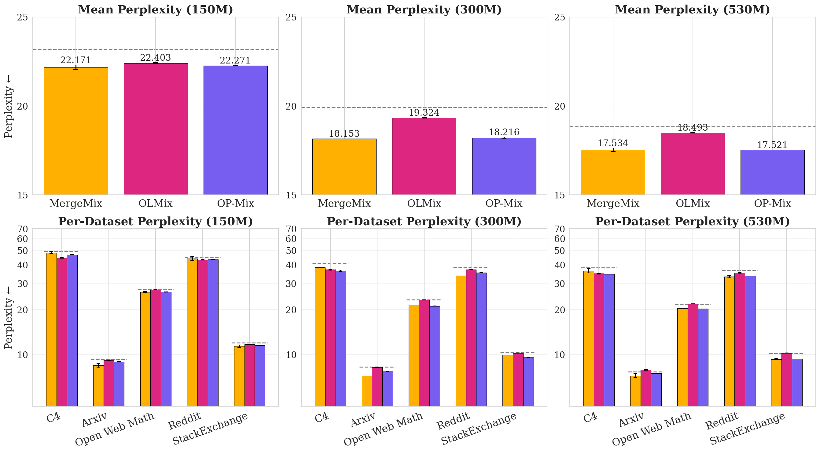
Pretraining (Figure 4).

We pretrain three different model sizes—150M, 300M, and 530M—from the OLMo model ladder ([27]) to Chinchilla-optimal ([28]) token counts of 3.2B, 6.5B, and 10.5B, respectively. We construct the pretraining data from 5 data domains: Algebraic Stack, ArXiv, c4, Reddit, and StackExchange ([29, 30]). During evaluation, we measure perplexity on all data domains and compute overall perplexity by a simple unweighted average. Each data domain contains more than 10.5B tokens, so no data mixture trains for more than one epoch on any data domain.

In pretraining, $\textsc{OP-Mix}$ matches the performance of MergeMix using up to 14% less compute (Figure 2 A) and outperforms OLMix by 5-6% at every scale. This is consistent with our on-policy hypothesis: $\textsc{OP-Mix}$ and MergeMix both build proxies from the model being trained, while OLMix uses a separate proxy whose learning dynamics diverge from the base model. These results are roughly mirrored by the downstream evaluations in Table 2 in Appendix, where $\textsc{OP-Mix}$ is either best or second-best in downstream task performance. Overall, $\textsc{OP-Mix}$ consistently outperforms ERM in perplexity and downstream evaluations while being more efficient than MergeMix.

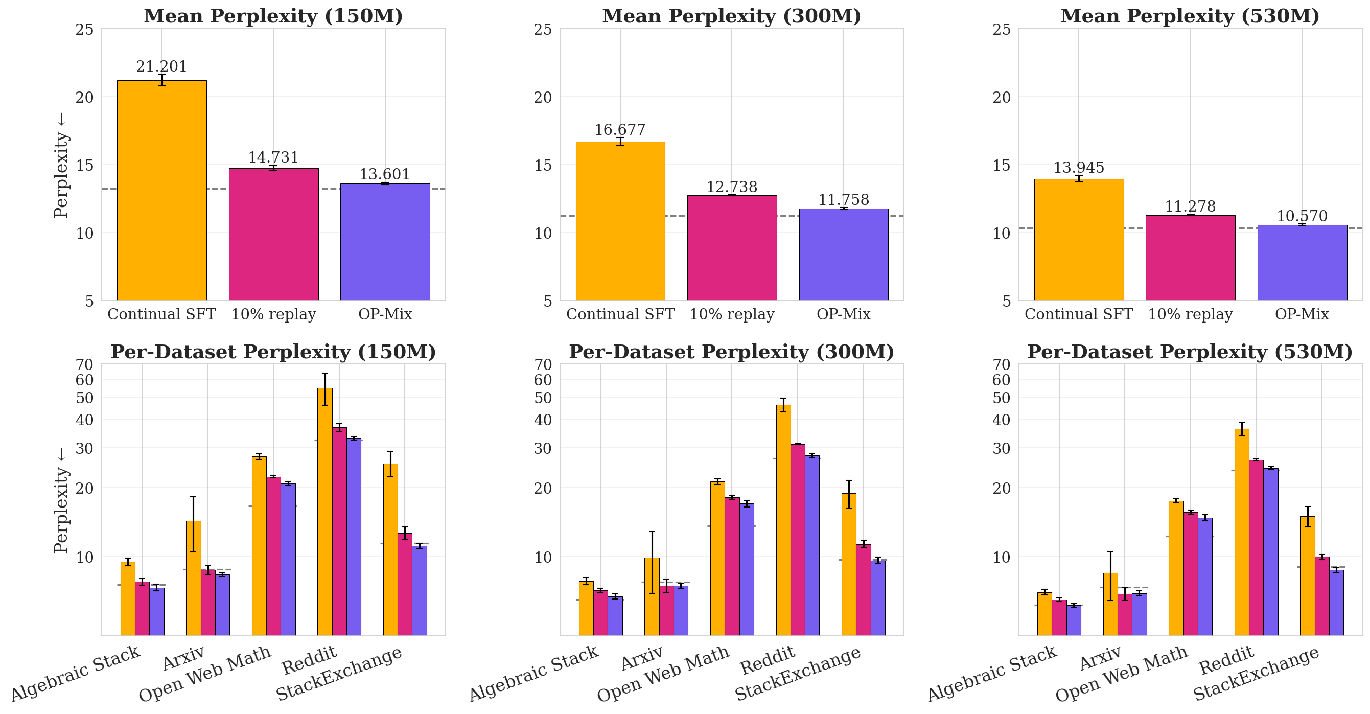
Continual Midtraining (Figure 5).

In continual midtraining, the user receives a stream of new data domains, emulating the real-life scenario where one updates a base model using new reference datasets. Here, our data mixture must expand per new dataset. In this section, we finetune open-source LMs pretrained on C4 ([29]) from the DataDecide model suite ([31]). We continually finetune models of parameter counts 150M, 300M, and 530M on Algebraic Stack, ArXiv, Open Web Math, Reddit, and StackExchange in alphabetic order. To account for ordering effects, we cyclically permute the order of the datasets so that each dataset appears once in every order position and train on all five combinations (see Table 6 in Appendix).

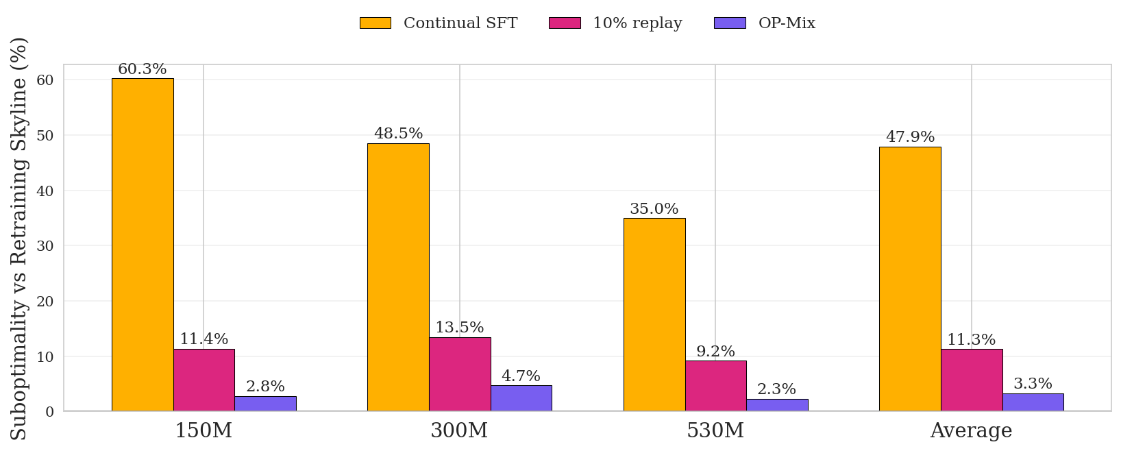
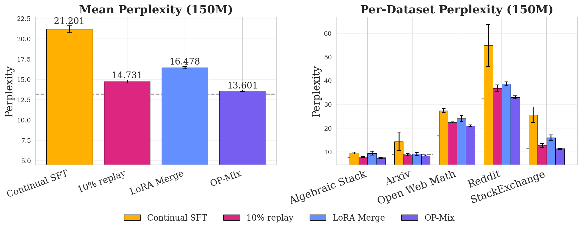
During continual midtraining, continual SFT suffers severe catastrophic forgetting (Figure 3), and of the data-mixing methods, $\textsc{OP-Mix}$ is best at mitigating it, nearly matching the performance of full retraining (Figure 9) while using up to 66% less compute. In Figure 10 (Appendix), we also include an ablation that merges in trained LoRAs into the base model using the optimized $\alpha^*$, instead of full finetuning. Although better than Continual SFT, LoRA-Merge is significantly worse than $\textsc{OP-Mix}$, indicating that there are benefits to using LoRA only as a proxy.

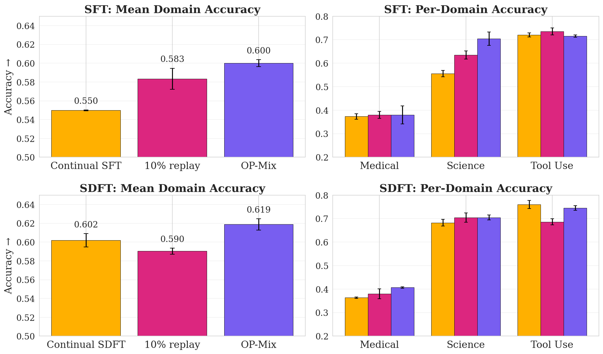
Continual Instruction Tuning (Figure 6).

We take the following continual learning task and ordering verbatim from [17]: we continually finetune Qwen2.5-7B-Instruct ([32]) on three instruction-following domains—Tool Use (4k examples), Science (1.2k examples), and Medical (10k examples)—introduced one at a time. In addition to standard SFT, we test Self-Distillation Finetuning (SDFT) ([17]) as the training objective. Performance is measured by mean accuracy across domains.

$\textsc{OP-Mix}$ on top of standard SFT (60.0%) matches the performance of SDFT (60.2%) while using 95% less compute, demonstrating that data mixing alone can recover the gains of a more sophisticated continual learning algorithm. (SDFT uses more compute as it repeatedly generates and distills on its own training data.) The two methods are also synergistic: combining $\textsc{OP-Mix}$ with SDFT achieves the best overall performance (61.9%), suggesting that data mixing and objective modifications are orthogonal axes of improvement.

4.2 Efficiency: $\textsc{OP-Mix}$ Pareto-Dominates on the Performance-Efficiency Frontier

Figure 2 (on page 2) compares methods by final performance versus total training FLOPs, counting both mixture selection and final training. $\textsc{OP-Mix}$ Pareto-dominates across pretraining, continual midtraining, and continual instruction tuning: no baseline achieves better performance at lower compute. $\textsc{OP-Mix}$ 's reuse of mixtures especially matters in continual midtraining (Figure 2 B), where the cost of naive retraining grows with every new domain. Unlike retraining, $\textsc{OP-Mix}$ turns adaptive data mixing into a lightweight operation that can be repeated whenever new data arrives.

5. Analysis

Section Summary: The analysis demonstrates that OP-Mix reliably identifies strong data mixtures, as the loss surface obtained by merging LoRA adapters closely matches the true surface from full training on those mixtures, incurring just a 0.9% average loss penalty versus the optimum. It then formalizes two sources of approximation error—replacing full fine-tuning with LoRA and using linear interpolation of weights instead of training on blended data—showing that the resulting performance gap is bounded by twice the sum of these errors. Empirical checks confirm the gap remains small and stable over successive stages, consistent with linear mode connectivity in models that share a common base.

5.1 $\textsc{OP-Mix}$ Reliably and Efficiently Estimates Optimal Data Mixtures

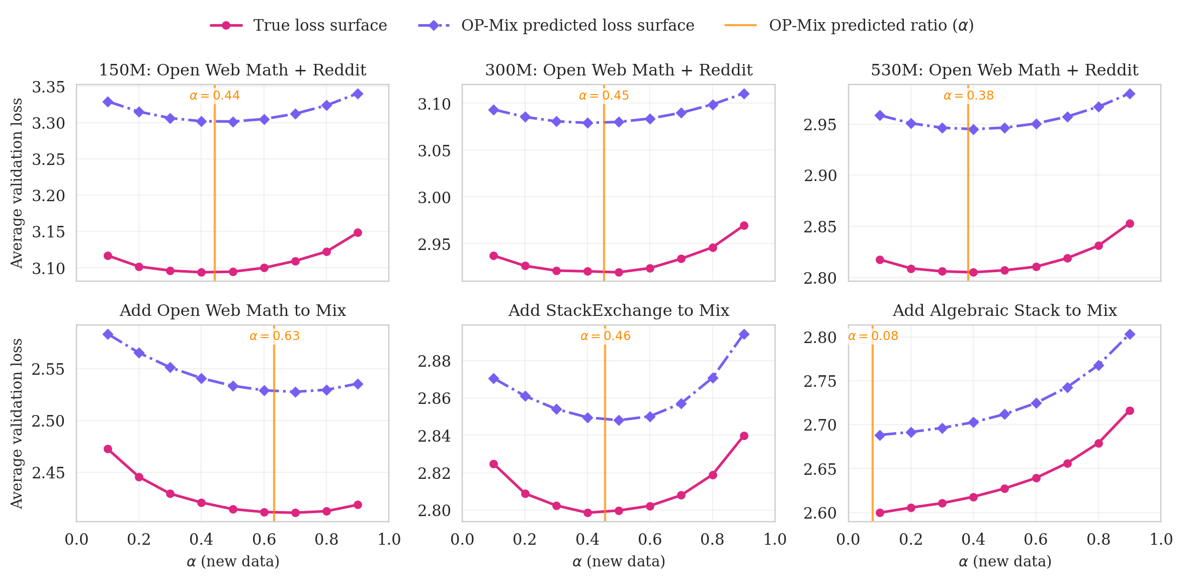
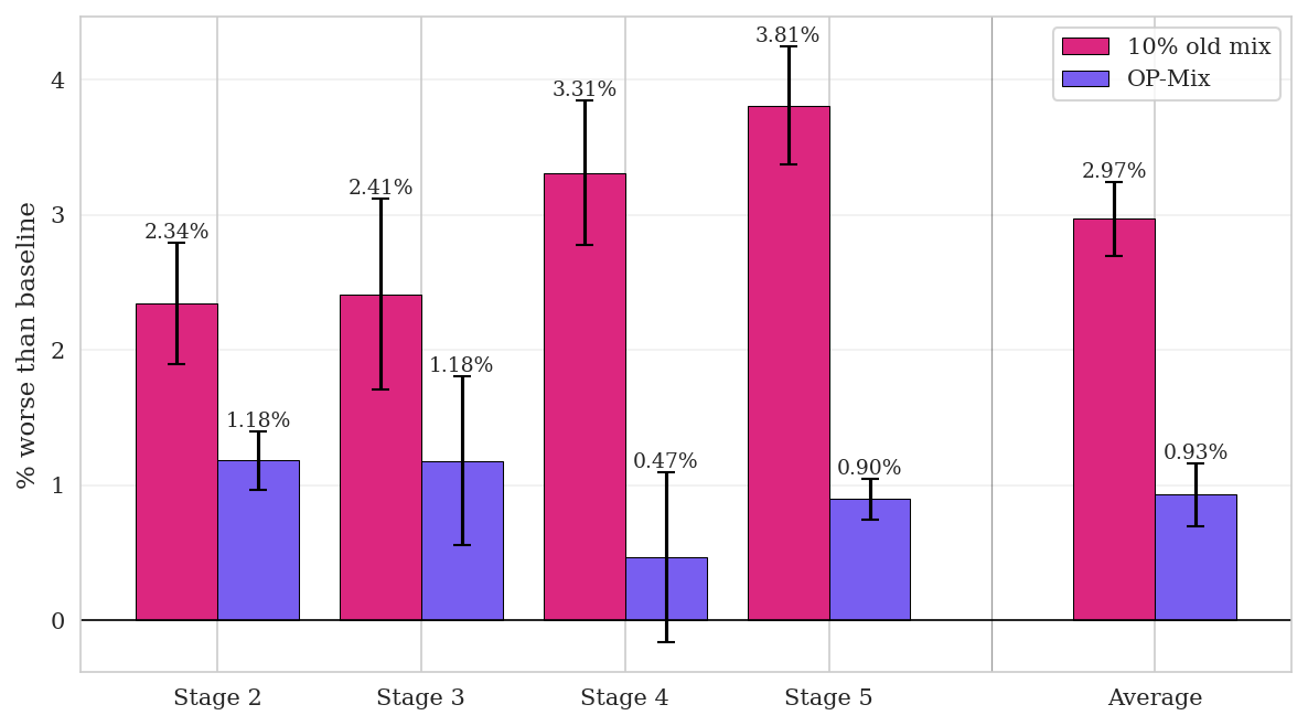
We ask whether $\textsc{OP-Mix}$ consistently recovers good mixing weights. In Figure 7, we plot the true loss surface with respect to mixture proportions in red and the estimated loss surface from $\textsc{OP-Mix}$ in purple. We generate the true loss surface by training on those proportions for all of training, as opposed to training a proxy. We find that merging LoRAs closely tracks the true data mixing loss surface. More concretely, in Figure 8 in the Appendix, we sweep for the best mixture at each stage in the continual midtraining setting and find that the average increase in loss of $\textsc{OP-Mix}$ from the optimal proportions is 0.9%, compared to a 2.9% increase for the fixed 10% data replay baseline.

5.2 Theoretical Analysis: Formalizing $\textsc{OP-Mix}$ 's Sources of Error

We now analyze the conditions under which $\textsc{OP-Mix}$ recovers an optimal interpolation weight, and bound the suboptimality of its predicted weight to the optimal weight. This section formalizes the intuition that $\textsc{OP-Mix}$ 's error is small if 1) LoRA performance is a good approximation of full fine-tuning performance and 2) linear interpolation is a good approximation for mixing.

Setup.

Suppose we receive a new domain $D_{m+1}$. Let $F(\alpha) = \frac{1}{N}\sum_{j=1}^{N} f_j(\theta^{\text{train}}(\alpha))$ denote the average evaluation performance of a model trained on the mixture assigning weight $\alpha \in [0, 1]$ to $D_{m+1}$ and distributing $1 - \alpha$ over previous domains $D_{\text{old}}$. $\textsc{OP-Mix}$ constructs a proxy for $F$ via two approximations: rather than training a full model on $D_{m+1}$, $\textsc{OP-Mix}$ trains two LoRA adapters $\theta^{\text{LoRA}}{D{m+1}}$ and $\theta^{\text{LoRA}}{D{\text{old}}}$; and rather than training on multiple data mixtures, $\textsc{OP-Mix}$ evaluates linear interpolations between the two LoRA adapters, yielding the proxy loss $\hat{F}(\alpha) = \frac{1}{N}\sum_{i=1}^N f_i!\left(\theta^{\text{LoRA}}(\alpha)\right)$.

To isolate the contributions of these two approximations, we follow [3] and define an intermediate surface $F^M(\alpha) = \frac{1}{N}\sum_{i=1}^N f_i(\theta^{\text{full}}(\alpha))$, where $\theta^{\text{full}}(\alpha) = (1-\alpha) \cdot \theta_{D_{\text{old}}} + \alpha \cdot\theta_{D_{m+1}}$ interpolates full finetuning updates instead of LoRAs. The two errors are then:

$ \varepsilon_{\text{merge}} := \sup_{\alpha \in [0, 1]} \left|F(\alpha) - F^M(\alpha)\right|, \quad \varepsilon_{\text{LoRA}} := \sup_{\alpha \in [0, 1]} \left|F^M(\alpha) - \hat{F}(\alpha)\right|. $

If both approximations are exact ($\varepsilon_{\mathrm{merge}} = \varepsilon_{\mathrm{LoRA}} = 0$), then $\textsc{OP-Mix}$ returns an optimal interpolation weight. When the approximations are imperfect, the following bound holds:

########## {caption="Remark 1: OP-Mix performance gap"}

Define the true regularized objective $J(\alpha) = F(\alpha) + \lambda , D_{\text{KL}}!\bigl(E(\boldsymbol{\alpha}) , \big|, \mu\bigr)$ and the proxy objective $\hat{J}(\alpha) = \hat{F}(\alpha) + \lambda , D_{KL}!\bigl(E(\boldsymbol{\alpha}) , \big|, \mu\bigr), $ and let $\alpha^\star \in \arg\min_{\alpha \in [0, 1]} J(\alpha)$ and $\hat{\alpha} \in \arg\min_{\alpha \in [0, 1]} \hat{J}(\alpha)$. Then:

$ J(\hat{\alpha}) - J(\alpha^\star) ;\le; 2!\left(\varepsilon_{merge} + \varepsilon_{LoRA}\right).\tag{1} $

Proof sketch: See Appendix B for full proof. The following holds:

$ J(\hat{\alpha}) - J(\alpha^\star) ;=; \underbrace{\big[J(\hat{\alpha}) - \hat{J}(\hat{\alpha})\big]}{\le, \varepsilon{merge} + \varepsilon_{LoRA}} ;+; \underbrace{\big[\hat{J}(\hat{\alpha}) - \hat{J}(\alpha^\star)\big]}{\le; 0} ;+; \underbrace{\big[\hat{J}(\alpha^\star) - J(\alpha^\star)\big]}{\le, \varepsilon_{merge} + \varepsilon_{LoRA}}. \nonumber $

The middle term is nonpositive because $\hat{\alpha}$ also minimizes $\hat{J}$. For the other two terms, the regularization terms cancel and the triangle inequality through $F^M$ gives $|F(\alpha) - \hat{F}(\alpha)| \le \varepsilon_{\mathrm{merge}} + \varepsilon_{\mathrm{LoRA}}$.

We verify empirically in Figure 8 that the overall approximation gap is small and non-increasing across continual learning stages. Furthermore, $\varepsilon_{\text{merge}}$ being small is empirically supported by linear mode connectivity ([33, 34]), which observes that linear interpolation does not incur large loss spikes when the finetuned models share a base model (see Corollary 7).

6. Related Work and Discussion

Section Summary: The section reviews continual learning research, which primarily tackles catastrophic forgetting of prior knowledge when models train on new data, through approaches like protecting parameters with regularization, replaying old examples, or adding model capacity. It also covers data mixing methods, including scaling laws that predict performance from mixture proportions via offline proxy models, as well as online algorithms that adapt mixtures during pretraining. The authors position OP-Mix as a novel replay-based technique that unifies mixing across training stages using efficient tools like LoRA and model merging, while acknowledging limits in scale and outlining extensions to larger models or reward-based training.

Continual learning.

The core challenge in continual learning is catastrophic forgetting, where training on new data degrades performance on previously learned tasks ([35]). Approaches to mitigating forgetting fall into three broad families: regularization-based methods constrain parameter updates to protect knowledge from earlier tasks ([36, 37]); replay-based methods retain or regenerate examples from previous tasks ([38, 39]); and architecture-based methods allocate new capacity for new tasks ([40, 41]). $\textsc{OP-Mix}$ is a replay-based method.

In the context of LLMs, forgetting can manifest across pretraining, instruction tuning, and alignment stages ([42, 43]). Our work considers in-weights learning, which updates model parameters. A parallel line of work keeps LLM weights frozen and accumulates knowledge in-context, e.g., via soft prompts ([44]) or modular KV-cache cartridges ([45]). However, the storage of in-context approaches grows with the dataset size, so amortizing knowledge from context to parameters using in-weights learning remains relevant.

Data mixing.

[1] established scaling laws for data mixtures, showing that downstream performance is a predictable function of mixture proportions. This empirically grounded the pipeline of training small proxy models on candidate mixtures and fitting a regression model to extrapolate to full scale ([2, 3]). In contrast to this offline approach, several online data mixing algorithms have been proposed for pretraining based on distributionally robust optimization, including DoReMi ([7]), DoGE ([5]) and GRAPE ([20]). [4] showed that both classes of algorithms are instances of the same linear framework.

Limitations and Future Work.

Our experiments top out at 530M parameters for pretraining and midtraining and 7B for instruction tuning, leaving open how $\textsc{OP-Mix}$ behaves at frontier scale (70B+ parameters). We also do not characterize how the LoRA proxy and model merging behave as the number of domains grows to 10 or 100. Future work can extend $\textsc{OP-Mix}$ to reward-based objectives like RLHF ([46]), where LoRA tends to work well ([47]). More broadly, our lifecycle-unification direction suggests that other training decisions, such as learning rate schedules or training objectives, may admit similarly unified formulations.

Conclusion.

The various phases of language model training are artificial divisions, and data mixing algorithms should work gracefully across them in a continual setting. Existing methods fall short on two fronts: they cannot incorporate new datasets, and they rely on off-policy proxy models. We address both limitations with $\textsc{OP-Mix}$, the first data mixing algorithm to achieve state-of-the-art results across pretraining, continual midtraining, and continual instruction tuning. By exploiting LoRA and linear mode connectivity to cheaply simulate candidate mixtures, $\textsc{OP-Mix}$ turns adaptive data mixing into a lightweight operation that can be repeated whenever new data arrives.

Acknowledgments

Section Summary: The authors thank several colleagues and the NYU Computation and Psycholinguistics Lab for helpful discussions and feedback on their work. Individual researchers received support through an NSF Graduate Research Fellowship and an Amazon AI PhD Fellowship. The project also drew on high-performance computing resources at NYU along with grants from Korean government institutes, Samsung, and multiple National Science Foundation awards.

We thank Graham Neubig, John Langford, Maxime Peyrard, Sebastian Cygert, Mayee Chen, and the NYU Computation and Psycholinguistics Lab for discussion and feedback. MYH is supported by the NSF Graduate Research Fellowship. AG is supported by the Amazon AI PhD Fellowship.

This work was supported in part through the NYU IT High Performance Computing resources, services, and staff expertise. This work was supported by the Institute of Information & Communications Technology Planning & Evaluation (IITP) with a grant funded by the Ministry of Science and ICT (MSIT) of the Republic of Korea in connection with the Global AI Frontier Lab International Collaborative Research. This work was also supported by the Samsung Advanced Institute of Technology (under the project Next Generation Deep Learning: From Pattern Recognition to AI) and the National Science Foundation (under NSF Awards 1922658, IIS-2239862, and IIS-2433429).

Appendix

Section Summary: The appendix presents additional figures, a performance table, and detailed reproducibility information for the OP-Mix method across pretraining and continual learning experiments. Figures compare OP-Mix against grid sweeps, full retraining, and simpler LoRA merging baselines on metrics like regret and downstream task performance, while Table 2 reports zero-shot accuracies for models of 150M to 530M parameters on benchmarks such as ARC, BoolQ, and MMLU. The reproducibility section lists shared hyperparameters like LoRA ranks and optimization settings, along with specifics for proxy construction and training schedules used in each experimental setting.

```latextable {caption="Table 2: Downstream zero-shot accuracy across ARC-Easy, ARC-Challenge ([48]), BoolQ ([49]), CommonsenseQA ([50]), HellaSwag ([51]), OpenBookQA ([52]), PIQA ([53]), WinoGrande ([54]), and MMLU ([55]), alongside their unweighted average. We ran evaluations using lm-eval-harness ([56]). Each block reports results for one model size. Bold marks the best result per column within each model size; italics mark the second best average score."} \begin{tabular}{l l c c c c c c c c c c} \toprule Size & Algorithm & ARC-E & ARC-C & BoolQ & CSQA & HSwag & OBQA & PIQA & WGrd & MMLU & Avg \ \midrule \multirow{4}{}{150M} & ERM & 33.57 & 20.85 & 56.72 & 19.49 & 27.08 & \textbf{24.60} & 58.27 & \textbf{51.04} & 23.01 & 34.96 \ & MergeMix & 33.26 & \textbf{21.76} & 60.05 & \textbf{19.52} & 27.37 & 23.93 & 57.85 & 50.72 & 23.00 & 35.28 \ & OLMix & 33.66 & \textbf{21.76} & \textbf{61.27} & 19.49 & 27.53 & 24.00 & \textbf{58.85} & 51.01 & 23.05 & \textbf{35.62} \ & OP-Mix & \textbf{33.68} & 21.16 & 59.92 & 19.49 & \textbf{27.62} & 23.93 & 58.34 & 50.49 & \textbf{23.07} & \textit{35.30} \ \midrule \multirow{4}{}{300M} & ERM & 34.82 & 21.53 & \textbf{60.18} & \textbf{19.60} & 28.29 & 25.33 & 59.45 & \textbf{51.33} & \textbf{23.06} & \textit{35.96} \ & MergeMix & 35.66 & 22.10 & 57.05 & 19.66 & 28.98 & 25.40 & 60.01 & 50.20 & 23.10 & 35.80 \ & OLMix & 35.90 & 21.56 & 54.10 & 19.49 & 28.80 & \textbf{25.80} & 60.39 & 50.59 & 23.04 & 35.52 \ & OP-Mix & \textbf{35.96} & \textbf{22.21} & 57.21 & 19.52 & \textbf{28.96} & 25.67 & \textbf{61.37} & 50.93 & \textbf{23.06} & \textbf{36.10} \ \midrule \multirow{4}{*}{530M} & ERM & 35.24 & 21.96 & 58.83 & 19.52 & 29.03 & 25.33 & 60.12 & 51.43 & 23.03 & 36.06 \ & MergeMix & \textbf{36.81} & \textbf{22.30} & 54.76 & \textbf{19.57} & 29.99 & \textbf{26.47} & \textbf{61.95} & 51.35 & \textbf{23.25} & 36.27 \ & OLMix & 36.41 & 21.99 & 59.04 & 19.44 & 29.54 & 26.13 & 61.43 & 50.83 & 23.12 & \textit{36.43} \ & OP-Mix & 36.59 & 21.99 & \textbf{61.45} & \textbf{19.57} & \textbf{30.13} & \textbf{26.47} & 61.15 & \textbf{51.78} & 23.10 & \textbf{36.91} \ \bottomrule \ \end{tabular}

### A. Reproducibility

#### A.1 Shared $\textsc{OP-Mix}$ configuration

Across all three settings, $\textsc{OP-Mix}$ uses the same high-level structure (Algorithm 1) and the same regression and solver. Shared choices are listed in Table 3.

: Table 3: Hyperparameters shared by $\textsc{OP-Mix}$  across pretraining, continual midtraining, and continual instruction tuning.

| Setting | Value |
| :--- | :--- |
| LoRA rank $r$ | 16 |
| LoRA scaling $\alpha$ | 32 |
| LoRA learning rate | 2× base finetuning LR |
| LoRA warmup | 0 steps |
| Regression form | log-linear per eval domain (fit via `cvxpy`) |
| Mix optimizer | `cvxpy` ([25]) on the reduced simplex $\triangle^{K}$ |
| Prior $\mu$ | uniform over the expanded domain set |
| KL regularization $\lambda$ | 0.05 |
| Base dtype | bfloat16 |
| Optimizer (base and LoRA) | AdamW, weight decay $0.01$ |
| LR schedule (base training) | WSD (warmup--stable--decay), 1000 decay steps |

The proxy construction differs slightly between settings. For pretraining, we Dirichlet-sample $P$ proxy mix vectors over $\{D_{\text{old}}, D_{m+1}, \dots, D_{m+K}\}$. For continual midtraining and continual instruction tuning, where $K=1$ new domain arrives per stage, we replace Dirichlet sampling with a deterministic 9-point grid over the old/new axis at $\alpha_{\text{new}} \in \{0.1, 0.2, \dots, 0.9\}$. In both continual settings the old- and new-domain LoRAs are trained with a *10/90* split (old probe mixes 10% of the new domain into the old mix; new probe mixes 10% of the old mix into the new domain) rather than one-hot specialization; we found this to prevent overestimation of forgetting while still being mathematically correct.

#### A.2 Pretraining

We pretrain from configuration-initialized OLMo models at three sizes on a five-domain mix of Algebraic Stack, ArXiv, c4, Reddit, and StackExchange, all tokenized with the DataDecide Dolma v1.5 tokenizer [31]. The model ladder uses the `allenai/DataDecide-c4-150M, 300M, 530M` architectures, initialized from config only (random weights). Per-size hyperparameters are in Table 4.

: Table 4: Pretraining hyperparameters for $\textsc{OP-Mix}$  and the ERM baseline. MergeMix uses the same prefix, proxy count, and probe length, but trains full-parameter proxies instead of LoRAs. OLMix uses a separate 20M-parameter proxy model (Table 5).

| | 150M | 300M | 530M |
| :--- | :---: | :---: | :---: |
| Base architecture | DataDecide-c4-150M | DataDecide-c4-300M | DataDecide-c4-530M |
| Total steps $R$ | 50, 000 | 50, 000 | 80, 000 |
| Global batch size | 32 | 64 | 64 |
| Sequence length | 1024 | 1024 | 1024 |
| Learning rate | $5\times10^{-4}$ | $4\times10^{-4}$ | $3\times10^{-4}$ |
| Warmup steps | 1, 000 | 5, 000 | 8, 000 |
| ERM warm start | 0.20 $R$ | 0.20 $R$ | 0.20 $R$ |
| LoRA steps | 5, 000 | 5, 000 | 5, 000 |
| Proxy points $P$ | 20 | 20 | 20 |

The ERM prefix is trained on the uniform mix $(1/5, 1/5, 1/5, 1/5, 1/5)$. After the prefix, each of the 5 LoRA probes is trained on a *90%-on-its-domain / 10%-on-the-old-mix* partition so the span of the 5 adapters covers the full simplex interior. We then build $P=20$ Dirichlet-sampled interpolation merges, evaluate each on the held-out shards of all 5 domains, fit the log-linear regression, and train for the remaining $0.8R$ steps on the fitted mix.

: Table 5: Proxy configuration for the OLMix baseline in pretraining.

| OLMix proxy (20M) | Value |
| :--- | :--- |
| Base architecture | DataDecide-c4-20M |
| Total steps | 10, 000 |
| Batch size | 32 |
| Learning rate | $1\times10^{-3}$ |
| Warmup steps | 5, 000 |
| Proxy mixtures | 64 Dirichlet samples |

#### A.3 Continual midtraining

We start from the pretrained DataDecide-c4 checkpoints from pretraining and continually finetune on the same five domains as pretraining, introduced one stage at a time. To control for ordering effects we run all five cyclic permutations `ord0` through `ord4` (Table 6).

: Table 6: Cyclic orderings of the five midtraining domains. Results are averaged across these five orderings.

| Ordering | Stage sequence |
| :--- | :--- |
| `ord0` | algebraic_stack $\to$ arxiv $\to$ open_web_math $\to$ reddit $\to$ stackexchange |
| `ord1` | arxiv $\to$ open_web_math $\to$ reddit $\to$ stackexchange $\to$ algebraic_stack |
| `ord2` | open_web_math $\to$ reddit $\to$ stackexchange $\to$ algebraic_stack $\to$ arxiv |
| `ord3` | reddit $\to$ stackexchange $\to$ algebraic_stack $\to$ arxiv $\to$ open_web_math |
| `ord4` | stackexchange $\to$ algebraic_stack $\to$ arxiv $\to$ open_web_math $\to$ reddit |

Per-stage hyperparameters are in Table 7. Every stage consists of two LoRA probes (old and new, with the 10/90 split above), a 9-point 1-D proxy scan, a `cvxpy` mix fit on the reduced $(\alpha_{\text{old}}, \alpha_{\text{new}})$ simplex, expansion of $\alpha_{\text{old}}^\star$ onto the previous stage's mix, and a full-model finetune on the expanded mix.

::: {caption="Table 7: Per-stage hyperparameters for continual midtraining. Stage 1 is a single-domain finetune; stages 2--5 run the full $\textsc{OP-Mix}$ pipeline on top of the previous stage's checkpoint."}

![](https://ittowtnkqtyixxjxrhou.supabase.co/storage/v1/object/public/public-images/d7rc5twq/complex_tab_1a8da96e7117.png)

:::

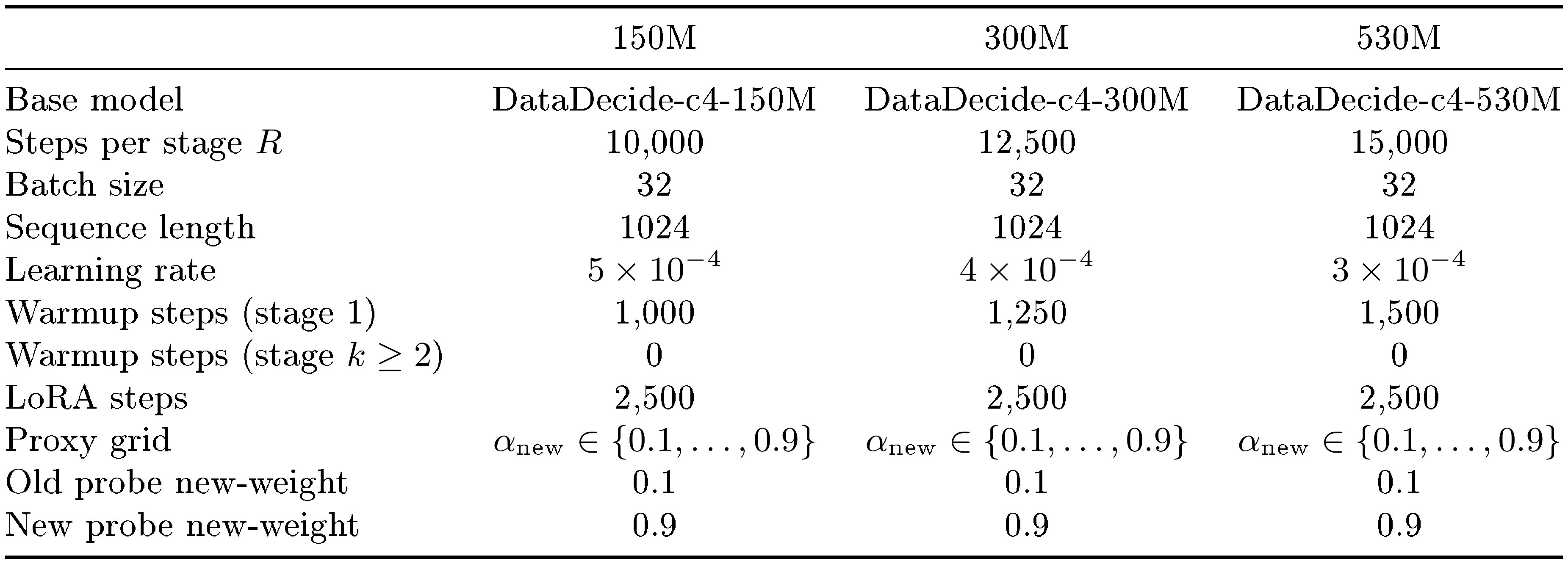
Baselines inherit the same $R$, batch size, sequence length, learning rate, and warmup schedule. The ``10% data replay'' baseline fixes $\alpha_{\text{old}}=0.1$ at every stage and expands onto the previous mix using the same expansion map $E$ as $\textsc{OP-Mix}$. ``Retrain'' trains from the original base model for $k\cdot R$ steps on the uniform mix over the $k$ domains seen so far.

#### A.4 Continual instruction tuning

We use Qwen2.5-7B-Instruct ([32]) as the base, and reuse the three domains and ordering of [17]: Tool Use (4,046 examples) $\to$ Science (1,233 examples) $\to$ Medical (10,000 examples). Each stage is one epoch over its dataset (capped at 10,000 examples). We evaluate with the SDFT accuracy metric of [17], averaged across the domains seen so far.

::: {caption="Table 8: Hyperparameters for the Qwen2.5-7B-Instruct continual instruction tuning experiments. The same settings are used for both the SFT and SDFT variants; SFT simply disables the SDFT-specific options. The LoRA probe is trained for a fixed 256 optimizer steps (short relative to the $\sim\!2{,}500$-step midtraining LoRA) because the instruction datasets here are small."}

![](https://ittowtnkqtyixxjxrhou.supabase.co/storage/v1/object/public/public-images/d7rc5twq/complex_tab_59fc1ca84eff.png)

:::

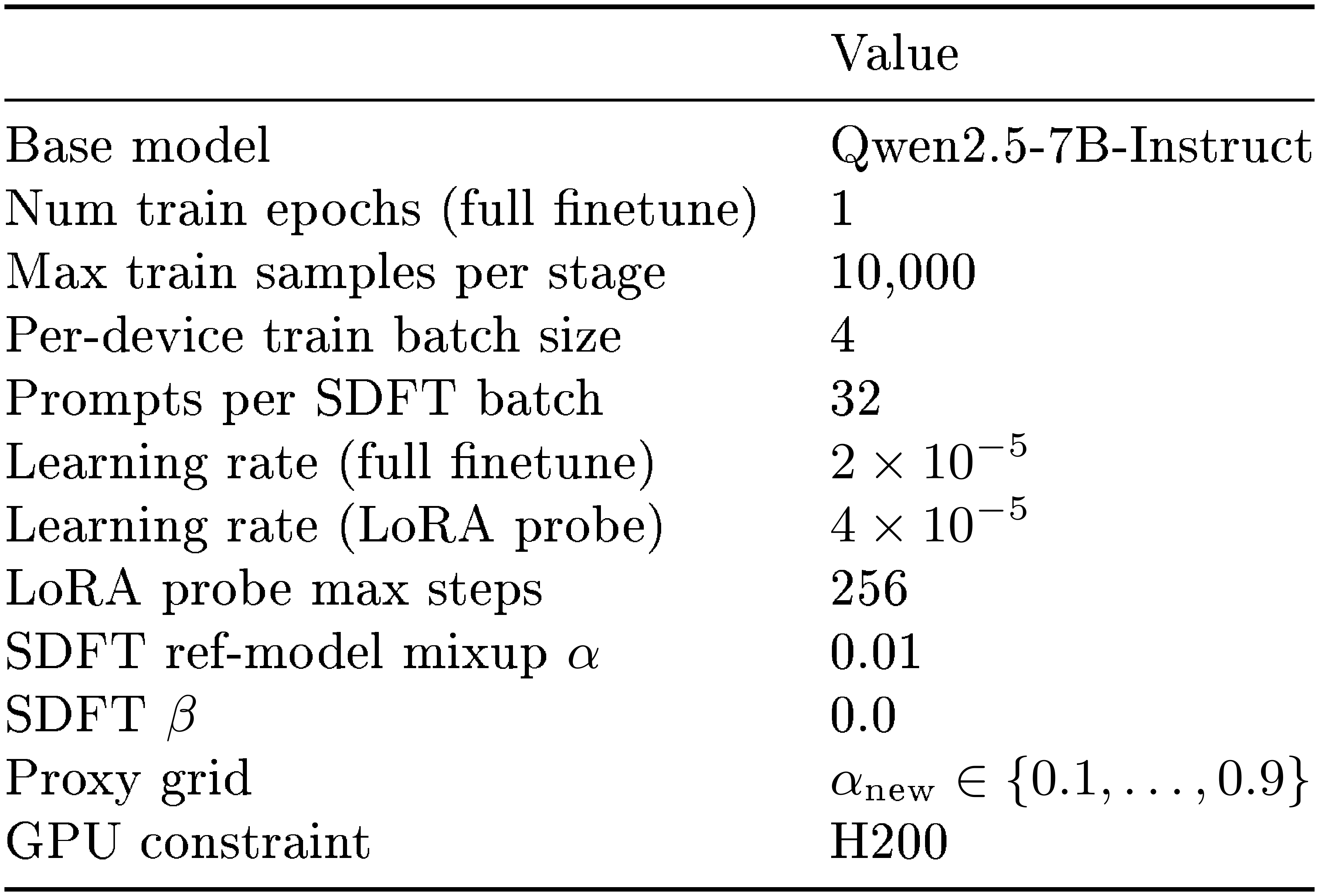
The difference between SFT and SDFT ([17]) is the training objective: SFT uses cross-entropy against the dataset targets, while SDFT replaces the targets with reverse KL-divergence to a teacher model's distribution. In the case of SDFT, the teacher is a moving average variant of the student that also receives the correct answer. In any case, $\textsc{OP-Mix}$ is applied identically on top of either objective: it only chooses the data-mix weights fed into the training loop, so ``SFT + $\textsc{OP-Mix}$ '' and ``SDFT + $\textsc{OP-Mix}$ '' use exactly the proxy, regression, and solver pipeline of Table 3, just with the respective loss.

**Compute.**

All experiments run on a cluster with a mix of A100, H100, L40S, and H200 GPUs. A nice property of LoRA is that it allows on-policy proxies to run on heterogeneous compute: for example, we can run pretraining on an H200 but run proxies on an L40S, which has less than a third of the GPU VRAM.

**Seeds and variance.**

Continual midtraining configuration is run for a single seed per model size, ordering cell; variance in the continual setting is instead quantified across the five cyclic orderings. Pretraining and continual instruction tuning results are both averaged across seeds $s \in \{42, 43, 44\}$.

### B. Theory

Consider one continual step of Algorithm 1. The current stage has previous domains $\{D_1, \dots, D_m\}$, over which we played the mixture $p_{t-1}\in\triangle^{m-1}$, and receives new domains $\{D_{m+1}, \dots, D_{m+K}\}$. Let

$
\boldsymbol{\alpha} = (\alpha_{\text{old}}, \alpha_{m+1}, \dots, \alpha_{m+K}) \in \triangle^{K}
$

denote the reduced-simplex weights used by $\textsc{OP-Mix}$, and let $E:\triangle^K \to \triangle^{m+K-1}$ be the mixture expansion map from Algorithm 1. We write $\theta_{\text{base}}$ for the current base model, and $\theta^{\text{train}}(\boldsymbol{\alpha})$ for the model obtained by continuing training from $\theta_{\text{base}}$ on the expanded mixture $E(\boldsymbol{\alpha})$.

For the proxy construction, let $\theta^{\text{full}}_{\text{old}}$ be the result of full finetuning on the old-data mixture $p_{t-1}$, and let $\theta^{\text{full}}_{D_{m+k}}$ be the result of full finetuning on $D_{m+k}$, all starting from $\theta_{\text{base}}$. Likewise, let $\theta^{\text{LoRA}}_{\text{old}}$ and $\theta^{\text{LoRA}}_{D_{m+k}}$ be the corresponding LoRA-adapted models produced by Algorithm 1, with the adapters applied to $\theta_{\text{base}}$. We then define the merged full-model proxy and merged LoRA proxy:

$
\begin{aligned}
\theta^M(\boldsymbol{\alpha}) &:= \alpha_{\text{old}}\theta^{\text{full}}_{\text{old}} + \sum_{k=1}^{K} \alpha_{m+k}\theta^{\text{full}}_{D_{m+k}}, \\
  \hat{\theta}(\boldsymbol{\alpha}) &:= \alpha_{\text{old}}\theta^{\text{LoRA}}_{\text{old}} + \sum_{k=1}^{K} \alpha_{m+k}\theta^{\text{LoRA}}_{D_{m+k}}.
\end{aligned}
$

Because the coefficients in $\boldsymbol{\alpha}$ sum to one and every model above is trained from the same $\theta_{\text{base}}$, these expressions are convex combinations of the corresponding parameter updates.

The three loss surfaces are therefore

$
\begin{aligned}
F(\boldsymbol{\alpha}) &:= \frac{1}{N}\sum_{j=1}^{N} f_j \!\left(\theta^{\text{train}}(\boldsymbol{\alpha})\right), \\
  F^M(\boldsymbol{\alpha}) &:= \frac{1}{N}\sum_{j=1}^{N} f_j \!\left(\theta^M(\boldsymbol{\alpha})\right), \\
  \hat{F}(\boldsymbol{\alpha}) &:= \frac{1}{N}\sum_{j=1}^{N} f_j \!\left(\hat{\theta}(\boldsymbol{\alpha})\right).
\end{aligned}
$

The regularized objectives are

$
\begin{aligned}
J(\boldsymbol{\alpha}) &:= F(\boldsymbol{\alpha}) + \lambda D_{\text{KL}} \! \bigl(E(\boldsymbol{\alpha})  \big \| \mu\bigr), \\
  \hat{J}(\boldsymbol{\alpha}) &:= \hat{F}(\boldsymbol{\alpha}) + \lambda D_{\text{KL}} \! \bigl(E(\boldsymbol{\alpha})  \big \| \mu\bigr),
\end{aligned}
$

with optimizers

$
\begin{aligned}
\boldsymbol{\alpha}^\star &:= \arg\min_{\boldsymbol{\alpha} \in \triangle^K} J(\boldsymbol{\alpha}), \\
  \hat{\boldsymbol{\alpha}} &:= \arg\min_{\boldsymbol{\alpha} \in \triangle^K} \hat{J}(\boldsymbol{\alpha}).
\end{aligned}
$

The two approximation errors are

$
\begin{aligned}
\varepsilon_{\text{merge}} &:= \sup_{\boldsymbol{\alpha} \in \triangle^K} \left|F(\boldsymbol{\alpha}) - F^M(\boldsymbol{\alpha})\right|, \\
  \varepsilon_{\text{LoRA}} &:= \sup_{\boldsymbol{\alpha} \in \triangle^K} \left| F^M(\boldsymbol{\alpha}) - \hat{F}(\boldsymbol{\alpha})\right|.
\end{aligned}
$

########## {caption="**Assumption 2**: Idealized proxy optimization"}

We assume: (i) the fitted regression surface used in Algorithm 1 recovers the merged-LoRA loss surface exactly, so the optimization step is equivalent to minimizing $\hat{J}$ over $\triangle^K$; and (ii) both $J$ and $\hat{J}$ are minimized exactly. This isolates the structural approximation errors induced by LoRA and model merging from finite-sample regression error, numerical optimization error, and proxy-training budget mismatch.

#### B.1 Exact Recovery

########## {caption="**Proposition 3**: Exact recovery"}

Under Assumption 2, if $\varepsilon_{\mathrm{merge}} = \varepsilon_{\mathrm{LoRA}} = 0$, then $\hat{F} = F$ on $\triangle^K$ and every minimizer of $\hat{J}$ is also a minimizer of $J$. In particular,

$
\hat{\boldsymbol{\alpha}} \in \arg\min_{\boldsymbol{\alpha} \in \triangle^K} J(\boldsymbol{\alpha}).
$

**Proof**: If $\varepsilon_{\mathrm{merge}} = 0$, then $F(\boldsymbol{\alpha}) = F^M(\boldsymbol{\alpha})$ for all $\boldsymbol{\alpha} \in \triangle^K$, so the merged full-model proxy matches the loss of training on the expanded mixture. If additionally $\varepsilon_{\mathrm{LoRA}} = 0$, then $F^M(\boldsymbol{\alpha}) = \hat{F}(\boldsymbol{\alpha})$ for all $\boldsymbol{\alpha}$, so the merged LoRA proxy is also exact. Hence $\hat{F}(\boldsymbol{\alpha}) = F(\boldsymbol{\alpha})$ on $\triangle^K$, which implies $\hat{J}(\boldsymbol{\alpha}) = J(\boldsymbol{\alpha})$ because both objectives share the same regularizer. Therefore $\arg\min \hat{J} = \arg\min J$, and in particular any optimizer $\hat{\boldsymbol{\alpha}}$ of the proxy objective is also an optimizer of the true objective.

This is the analog of Lemma 2 of [3], which shows exact recovery when the reused mixture is itself optimal. For $\textsc{OP-Mix}$, the corresponding ideal condition is that the reduced-simplex proxy surface exactly matches the true objective after expansion by $E$.

#### B.2 Performance Gap Bound

We first establish a uniform approximation lemma, then use it to prove Equation 1.

########## {caption="**Lemma 4**: Uniform proxy error"}

For any $\boldsymbol{\alpha} \in \triangle^K$:

$
\left|F(\boldsymbol{\alpha}) - \hat{F}(\boldsymbol{\alpha})\right| \;\le\; \varepsilon_{merge} + \varepsilon_{LoRA}.
$

**Proof**: By the triangle inequality, introducing the intermediate surface $F^M$:

$
\begin{aligned}
\left|F(\boldsymbol{\alpha}) - \hat{F}(\boldsymbol{\alpha})\right| &= \left|F(\boldsymbol{\alpha}) - F^M(\boldsymbol{\alpha}) + F^M(\boldsymbol{\alpha}) - \hat{F}(\boldsymbol{\alpha})\right| \nonumber \\
  &\le \left|F(\boldsymbol{\alpha}) - F^M(\boldsymbol{\alpha})\right| + \left|F^M(\boldsymbol{\alpha}) - \hat{F}(\boldsymbol{\alpha})\right| \nonumber \\
  &\le \sup_{\boldsymbol{\alpha}' \in \triangle^K} \left|F(\boldsymbol{\alpha}') - F^M(\boldsymbol{\alpha}')\right| + \sup_{\boldsymbol{\alpha}' \in \triangle^K} \left|F^M(\boldsymbol{\alpha}') - \hat{F}(\boldsymbol{\alpha}')\right| \nonumber \\
  &= \varepsilon_{merge} + \varepsilon_{LoRA}. \nonumber \blacksquare
\end{aligned}
$

########## {caption="**Remark**: OP-Mix performance gap, full proof"}

Under Assumption 2:

$
J(\hat{\boldsymbol{\alpha}}) - J(\boldsymbol{\alpha}^\star) \;\le\; 2\!\left(\varepsilon_{merge} + \varepsilon_{LoRA}\right). \tag{Equation 1}
$

**Proof**: We decompose the objective gap by adding and subtracting $\hat{J}$:

$
\begin{aligned}
J(\hat{\boldsymbol{\alpha}}) - J(\boldsymbol{\alpha}^\star) &= \big[J(\hat{\boldsymbol{\alpha}}) - \hat{J}(\hat{\boldsymbol{\alpha}})\big] + \big[\hat{J}(\hat{\boldsymbol{\alpha}}) - \hat{J}(\boldsymbol{\alpha}^\star)\big] + \big[\hat{J}(\boldsymbol{\alpha}^\star) - J(\boldsymbol{\alpha}^\star)\big].
\end{aligned}\tag{2}
$

**Middle term.** Since $\hat{\boldsymbol{\alpha}} = \arg\min_{\boldsymbol{\alpha} \in \triangle^K} \hat{J}(\boldsymbol{\alpha})$ and $\boldsymbol{\alpha}^\star \in \triangle^K$:

$
\hat{J}(\hat{\boldsymbol{\alpha}}) - \hat{J}(\boldsymbol{\alpha}^\star) \;\le\; 0.\tag{3}
$

**First term.** Note that $J(\boldsymbol{\alpha}) - \hat{J}(\boldsymbol{\alpha}) = F(\boldsymbol{\alpha}) - \hat{F}(\boldsymbol{\alpha})$ for any $\boldsymbol{\alpha}$, since the regularization terms are identical in $J$ and $\hat{J}$. Applying Lemma 4:

$
J(\hat{\boldsymbol{\alpha}}) - \hat{J}(\hat{\boldsymbol{\alpha}}) = F(\hat{\boldsymbol{\alpha}}) - \hat{F}(\hat{\boldsymbol{\alpha}}) \;\le\; \left|F(\hat{\boldsymbol{\alpha}}) - \hat{F}(\hat{\boldsymbol{\alpha}})\right| \;\le\; \varepsilon_{merge} + \varepsilon_{LoRA}.\tag{4}
$

**Third term.** By the same reasoning:

$
\hat{J}(\boldsymbol{\alpha}^\star) - J(\boldsymbol{\alpha}^\star) = \hat{F}(\boldsymbol{\alpha}^\star) - F(\boldsymbol{\alpha}^\star) \;\le\; \left|\hat{F}(\boldsymbol{\alpha}^\star) - F(\boldsymbol{\alpha}^\star)\right| \;\le\; \varepsilon_{merge} + \varepsilon_{LoRA}.\tag{5}
$

Substituting Equation 3, Equation 4, and 5 into Equation 2:

$
\begin{aligned}
J(\hat{\boldsymbol{\alpha}}) - J(\boldsymbol{\alpha}^\star) &\;\le\; (\varepsilon_{merge} + \varepsilon_{LoRA}) + 0 + (\varepsilon_{merge} + \varepsilon_{LoRA}) \nonumber \\
  &\;=\; 2(\varepsilon_{merge} + \varepsilon_{LoRA}). \nonumber \blacksquare
\end{aligned}
$

#### B.3 Characterizing the Approximation Errors

The bound in Equation 1 reduces the analysis of $\textsc{OP-Mix}$ to bounding $\varepsilon_{\mathrm{merge}}$ and $\varepsilon_{\mathrm{LoRA}}$ separately. We now provide Lipschitz-based characterizations of each.

########## {caption="**Proposition 5**: LoRA approximation bound"}

If each downstream metric $f_j$ is $L_j$-Lipschitz in model parameters with respect to the Frobenius norm, i.e., $|f_j(\theta) - f_j(\theta')| \le L_j \|\theta - \theta'\|_F$ for all $\theta, \theta'$, then with $L = \frac{1}{N}\sum_{j=1}^N L_j$:

$
\varepsilon_{LoRA} \;\le\; L \cdot \max \! \Biggl\{
  \left\| \theta^{full}_{old} - \theta^{LoRA}_{old}\right \|_F, \;
  \max_{k \in [K]} \left\| \theta^{full}_{D_{m+k}} - \theta^{LoRA}_{D_{m+k}}\right \|_F
  \Biggr\}.\tag{6}
$

**Proof**: For any $\boldsymbol{\alpha} \in \triangle^K$:

$
\begin{aligned}
\left|F^M(\boldsymbol{\alpha}) - \hat{F}(\boldsymbol{\alpha})\right| &= \left|\frac{1}{N}\sum_{j=1}^N \Big[f_j\!\big(\theta^M(\boldsymbol{\alpha})\big) - f_j\!\big(\hat{\theta}(\boldsymbol{\alpha})\big)\Big]\right| \nonumber \\
  &\le \frac{1}{N}\sum_{j=1}^N L_j \left\|\theta^M(\boldsymbol{\alpha}) - \hat{\theta}(\boldsymbol{\alpha})\right\|_F \nonumber \\
  &= L \left\|\alpha_{old} \Big(\theta^{full}_{old} - \theta^{LoRA}_{old}\Big) + \sum_{k=1}^K \alpha_{m+k} \Big(\theta^{full}_{D_{m+k}} - \theta^{LoRA}_{D_{m+k}}\Big)\right\|_F \nonumber \\
  &\le L \left[\alpha_{old} \left\|\theta^{full}_{old} - \theta^{LoRA}_{old}\right\|_F + \sum_{k=1}^K \alpha_{m+k} \left\|\theta^{full}_{D_{m+k}} - \theta^{LoRA}_{D_{m+k}}\right\|_F \right] \nonumber \\
  &\le L \cdot \max\!\Biggl\{
  \left\|\theta^{full}_{old} - \theta^{LoRA}_{old}\right\|_F, \;
  \max_{k \in [K]} \left\|\theta^{full}_{D_{m+k}} - \theta^{LoRA}_{D_{m+k}}\right\|_F
  \Biggr\}. \blacksquare
\end{aligned}
$

########## {caption="**Proposition 6**: Merging approximation bound"}

Under the same Lipschitz condition as Proposition 5, let $\theta^{\mathrm{train}}(\boldsymbol{\alpha})$ denote the model trained on the expanded mixture $E(\boldsymbol{\alpha})$, and let $\theta^M(\boldsymbol{\alpha})$ denote the merged full-model proxy. Then:

$
\varepsilon_{merge} \;\le\; L \cdot \sup_{\boldsymbol{\alpha} \in \triangle^K} \left\|\theta^{train}(\boldsymbol{\alpha}) - \theta^M(\boldsymbol{\alpha})\right\|_F.\tag{7}
$

**Proof**: For any $\boldsymbol{\alpha} \in \triangle^K$:

$
\begin{aligned}
\left|F(\boldsymbol{\alpha}) - F^M(\boldsymbol{\alpha})\right| &= \left|\frac{1}{N}\sum_{j=1}^N \Big[f_j\!\big(\theta^{train}(\boldsymbol{\alpha})\big) - f_j\!\big(\theta^M(\boldsymbol{\alpha})\big)\Big]\right| \nonumber \\
  &\le \frac{1}{N}\sum_{j=1}^N L_j \left\|\theta^{train}(\boldsymbol{\alpha}) - \theta^M(\boldsymbol{\alpha})\right\|_F \nonumber \\
  &= L \left\|\theta^{train}(\boldsymbol{\alpha}) - \theta^M(\boldsymbol{\alpha})\right\|_F. \nonumber
\end{aligned}
$

Taking the supremum over $\boldsymbol{\alpha}$ yields the result.

########## {caption="**Corollary 7**: Merging error vanishes under linear mode connectivity"}

Define the linearity gap

$
\delta_{\mathrm{LMC}} := \sup_{\boldsymbol{\alpha} \in \triangle^K} \left\|\theta^{\mathrm{train}}(\boldsymbol{\alpha}) - \theta^M(\boldsymbol{\alpha})\right\|_F.
$

For any $\varepsilon > 0$, if $\delta_{\mathrm{LMC}} \le \varepsilon / L$, then $\varepsilon_{\mathrm{merge}} \le \varepsilon$.

**Proof**: $\varepsilon_{\mathrm{merge}} \le L \cdot \delta_{\mathrm{LMC}} \le L \cdot \varepsilon / L = \varepsilon$.

The linearity gap $\delta_{\mathrm{LMC}}$ measures how well the convex hull of the old-data model and the new-domain models approximates actual training on the expanded mixture. Because $\textsc{OP-Mix}$ compresses all historical data into the single component $\theta^{\mathrm{full}}_{\mathrm{old}}$, it only needs this reduced simplex to be well behaved, rather than requiring one separately trained model for every historical domain.

Linear mode connectivity says that moving along the interpolation path between endpoint models does not create a large loss barrier. That observation is exactly why model merging is a plausible proxy in $\textsc{OP-Mix}$: it suggests that linear interpolation should not cause catastrophic loss blowups.

## References

> **Section Summary**: This references section lists dozens of academic papers, technical reports, and preprints that support a study on training and optimizing large language models. Most citations focus on recent methods for mixing and reweighting training data, along with related techniques such as model merging, distillation, and scaling laws, drawn from conferences like ICLR, NeurIPS, and ICML as well as arXiv. Foundational works on models including BERT and GPT, plus reports on systems like Llama, Gemma, and OLMo, are also included to provide broader context.


[1] Jiasheng Ye et al. (2025). *Data Mixing Laws: Optimizing Data Mixtures by Predicting Language Modeling Performance*. In *The Thirteenth International Conference on Learning Representations*. [https://openreview.net/forum?id=jjCB27TMK3](https://openreview.net/forum?id=jjCB27TMK3).

[2] Qian Liu et al. (2025). *RegMix: Data Mixture as Regression for Language Model Pre-training*. In *The Thirteenth International Conference on Learning Representations*. [https://openreview.net/forum?id=5BjQOUXq7i](https://openreview.net/forum?id=5BjQOUXq7i).

[3] Chen et al. (2026). *Olmix: A Framework for Data Mixing Throughout LM Development*. arXiv preprint arXiv:2602.12237.

[4] Mayee F Chen et al. (2025). *Aioli: A Unified Optimization Framework for Language Model Data Mixing*. In *The Thirteenth International Conference on Learning Representations*. [https://openreview.net/forum?id=sZGZJhaNSe](https://openreview.net/forum?id=sZGZJhaNSe).

[5] Simin Fan et al. (2024). *DOGE: Domain Reweighting with Generalization Estimation*. In *Forty-first International Conference on Machine Learning*. [https://openreview.net/forum?id=7rfZ6bMZq4](https://openreview.net/forum?id=7rfZ6bMZq4).

[6] Yiding Jiang et al. (2025). *Adaptive Data Optimization: Dynamic Sample Selection with Scaling Laws*. In *The Thirteenth International Conference on Learning Representations*. [https://openreview.net/forum?id=aqok1UX7Z1](https://openreview.net/forum?id=aqok1UX7Z1).

[7] Sang Michael Xie et al. (2023). *DoReMi: Optimizing Data Mixtures Speeds Up Language Model Pretraining*. In *Thirty-seventh Conference on Neural Information Processing Systems*. [https://openreview.net/forum?id=lXuByUeHhd](https://openreview.net/forum?id=lXuByUeHhd).

[8] Chen et al. (2023). *Skill-it! a data-driven skills framework for understanding and training language models*. In *Proceedings of the 37th International Conference on Neural Information Processing Systems*.

[9] Edward J Hu et al. (2022). *LoRA: Low-Rank Adaptation of Large Language Models*. In *International Conference on Learning Representations*. [https://openreview.net/forum?id=nZeVKeeFYf9](https://openreview.net/forum?id=nZeVKeeFYf9).

[10] Jiapeng Wang et al. (2026). *MergeMix: Optimizing Mid-Training Data Mixtures via Learnable Model Merging*. [https://arxiv.org/abs/2601.17858](https://arxiv.org/abs/2601.17858). arXiv:2601.17858.

[11] Zhixu Silvia Tao et al. (2025). *Merge to Mix: Mixing Datasets via Model Merging*. [https://arxiv.org/abs/2505.16066](https://arxiv.org/abs/2505.16066). arXiv:2505.16066.

[12] Radford et al. (2019). *Language models are unsupervised multitask learners*. OpenAI blog. 1(8). pp. 9.

[13] Jacob Devlin et al. (2019). *BERT: Pre-training of Deep Bidirectional Transformers for Language Understanding*. [https://arxiv.org/abs/1810.04805](https://arxiv.org/abs/1810.04805). arXiv:1810.04805.

[14] Team OLMo et al. (2025). *2 OLMo 2 Furious*. [https://arxiv.org/abs/2501.00656](https://arxiv.org/abs/2501.00656). arXiv:2501.00656.

[15] Emmy Liu et al. (2026). *Midtraining Bridges Pretraining and Posttraining Distributions*. [https://arxiv.org/abs/2510.14865](https://arxiv.org/abs/2510.14865). arXiv:2510.14865.

[16] Jason Wei et al. (2022). *Finetuned Language Models are Zero-Shot Learners*. In *International Conference on Learning Representations*. [https://openreview.net/forum?id=gEZrGCozdqR](https://openreview.net/forum?id=gEZrGCozdqR).

[17] Idan Shenfeld et al. (2026). *Self-Distillation Enables Continual Learning*. [https://arxiv.org/abs/2601.19897](https://arxiv.org/abs/2601.19897). arXiv:2601.19897.

[18] Lu, Kevin (2025). *On-policy distillation*. Thinking Machines Lab: Connectionism.

[19] Zhao et al. (2026). *Self-Distilled Reasoner: On-Policy Self-Distillation for Large Language Models*. arXiv preprint arXiv:2601.18734.

[20] Simin Fan et al. (2025). *GRAPE: Optimize Data Mixture for Group Robust Multi-target Adaptive Pretraining*. In *The Thirty-ninth Annual Conference on Neural Information Processing Systems*. [https://openreview.net/forum?id=JRmIvBcnWc](https://openreview.net/forum?id=JRmIvBcnWc).

[21] Gemma Team et al. (2025). *Gemma 3 Technical Report*. [https://arxiv.org/abs/2503.19786](https://arxiv.org/abs/2503.19786). arXiv:2503.19786.

[22] Aaron Grattafiori et al. (2024). *The Llama 3 Herd of Models*. [https://arxiv.org/abs/2407.21783](https://arxiv.org/abs/2407.21783). arXiv:2407.21783.

[23] An Yang et al. (2025). *Qwen3 Technical Report*. [https://arxiv.org/abs/2505.09388](https://arxiv.org/abs/2505.09388). arXiv:2505.09388.

[24] Kaiyue Wen et al. (2025). *Understanding Warmup-Stable-Decay Learning Rates: A River Valley Loss Landscape View*. In *The Thirteenth International Conference on Learning Representations*. [https://openreview.net/forum?id=m51BgoqvbP](https://openreview.net/forum?id=m51BgoqvbP).

[25] Steven Diamond and Stephen Boyd (2016). *CVXPY: A Python-embedded modeling language for convex optimization*. Journal of Machine Learning Research. 17(83). pp. 1–5.

[26] Louis Béthune et al. (2025). *Scaling Laws for Forgetting during Finetuning with Pretraining Data Injection*. In *Forty-second International Conference on Machine Learning*. [https://openreview.net/forum?id=vWMij23BmQ](https://openreview.net/forum?id=vWMij23BmQ).

[27] Groeneveld et al. (2024). *OLMo: Accelerating the Science of Language Models*. In *Proceedings of the 62nd Annual Meeting of the Association for Computational Linguistics (Volume 1: Long Papers)*. pp. 15789–15809. doi:10.18653/v1/2024.acl-long.841. [https://aclanthology.org/2024.acl-long.841/](https://aclanthology.org/2024.acl-long.841/).

[28] Hoffmann et al. (2022). *Training compute-optimal large language models*. arXiv preprint arXiv:2203.15556. 10.

[29] Colin Raffel et al. (2020). *Exploring the Limits of Transfer Learning with a Unified Text-to-Text Transformer*. Journal of Machine Learning Research. 21(140). pp. 1–67. [http://jmlr.org/papers/v21/20-074.html](http://jmlr.org/papers/v21/20-074.html).

[30] Maurice Weber et al. (2024). *RedPajama: an Open Dataset for Training Large Language Models*. [https://arxiv.org/abs/2411.12372](https://arxiv.org/abs/2411.12372). arXiv:2411.12372.

[31] Ian Magnusson et al. (2025). *DataDecide: How to Predict Best Pretraining Data with Small Experiments*. In *Forty-second International Conference on Machine Learning*. [https://openreview.net/forum?id=p9YlQPF8fE](https://openreview.net/forum?id=p9YlQPF8fE).

[32] An Yang et al. (2024). *Qwen2 Technical Report*. [https://arxiv.org/abs/2407.10671](https://arxiv.org/abs/2407.10671). arXiv:2407.10671.

[33] Frankle et al. (2020). *Linear mode connectivity and the lottery ticket hypothesis*. In *Proceedings of the 37th International Conference on Machine Learning*.

[34] Wortsman et al. (2022). *Model soups: averaging weights of multiple fine-tuned models improves accuracy without increasing inference time*. In *Proceedings of the 39th International Conference on Machine Learning*. pp. 23965–23998. [https://proceedings.mlr.press/v162/wortsman22a.html](https://proceedings.mlr.press/v162/wortsman22a.html).

[35] Michael McCloskey and Neal J. Cohen (1989). *Catastrophic Interference in Connectionist Networks: The Sequential Learning Problem*. doi:https://doi.org/10.1016/S0079-7421(08)60536-8. [https://www.sciencedirect.com/science/article/pii/S0079742108605368](https://www.sciencedirect.com/science/article/pii/S0079742108605368).

[36] James Kirkpatrick et al. (2017). *Overcoming catastrophic forgetting in neural networks*. Proceedings of the National Academy of Sciences. 114(13). pp. 3521-3526. doi:10.1073/pnas.1611835114. [https://www.pnas.org/doi/abs/10.1073/pnas.1611835114](https://www.pnas.org/doi/abs/10.1073/pnas.1611835114).

[37] Aljundi et al. (2018). *Memory Aware Synapses: Learning What (not) to Forget*. In *Computer Vision – ECCV 2018: 15th European Conference, Munich, Germany, September 8–14, 2018, Proceedings, Part III*. pp. 144–161. doi:10.1007/978-3-030-01219- $9_9. [$ https://doi.org/10.1007/978-3-030-01219- $9_9]($ https://doi.org/10.1007/978-3-030-01219-$9_9)$.

[38] Rolnick et al. (2019). *Experience Replay for Continual Learning*. In *Advances in Neural Information Processing Systems*. pp. . [https://proceedings.neurips.cc/paper_files/paper/2019/file/fa7cdfad1a5aaf8370ebeda47a1ff1c3-Paper.pdf](https://proceedings.neurips.cc/paper_files/paper/2019/file/fa7cdfad1a5aaf8370ebeda47a1ff1c3-Paper.pdf).

[39] Shin et al. (2017). *Continual learning with deep generative replay*. In *Proceedings of the 31st International Conference on Neural Information Processing Systems*. pp. 2994–3003.

[40] Andrei A. Rusu et al. (2022). *Progressive Neural Networks*. [https://arxiv.org/abs/1606.04671](https://arxiv.org/abs/1606.04671). arXiv:1606.04671.

[41] Wang et al. (2023). *Orthogonal Subspace Learning for Language Model Continual Learning*. In *Findings of the Association for Computational Linguistics: EMNLP 2023*. pp. 10658–10671. doi:10.18653/v1/2023.findings-emnlp.715. [https://aclanthology.org/2023.findings-emnlp.715/](https://aclanthology.org/2023.findings-emnlp.715/).

[42] Shi et al. (2025). *Continual Learning of Large Language Models: A Comprehensive Survey*. ACM Comput. Surv.. 58(5). doi:10.1145/3735633. [https://doi.org/10.1145/3735633](https://doi.org/10.1145/3735633).

[43] Junhao Zheng et al. (2025). *Spurious Forgetting in Continual Learning of Language Models*. In *The Thirteenth International Conference on Learning Representations*. [https://openreview.net/forum?id=ScI7IlKGdI](https://openreview.net/forum?id=ScI7IlKGdI).

[44] Anastasia Razdaibiedina et al. (2023). *Progressive Prompts: Continual Learning for Language Models*. In *The Eleventh International Conference on Learning Representations*. [https://openreview.net/forum?id=UJTgQBc9 $1_]($ https://openreview.net/forum?id=UJTgQBc9$1_)$.

[45] Sabri Eyuboglu et al. (2026). *Cartridges: Lightweight and general-purpose long context representations via self-study*. In *The Fourteenth International Conference on Learning Representations*. [https://openreview.net/forum?id=0k5w8O0SNg](https://openreview.net/forum?id=0k5w8O0SNg).

[46] Long Ouyang et al. (2022). *Training language models to follow instructions with human feedback*. In *Advances in Neural Information Processing Systems*. [https://openreview.net/forum?id=TG8KACxEON](https://openreview.net/forum?id=TG8KACxEON).

[47] Schulman, John (2025). *LoRA Without Regret*. [https://thinkingmachines.ai/blog/lora/](https://thinkingmachines.ai/blog/lora/). Thinking Machines Lab blog post. In collaboration with others at Thinking Machines.

[48] Peter Clark et al. (2018). *Think you have Solved Question Answering? Try ARC, the AI2 Reasoning Challenge*. ArXiv. abs/1803.05457.

[49] Christopher Clark et al. (2019). *BoolQ: Exploring the Surprising Difficulty of Natural Yes/No Questions*. In *NAACL*.

[50] Talmor et al. (2019). *CommonsenseQA: A Question Answering Challenge Targeting Commonsense Knowledge*. In *Proceedings of the 2019 Conference of the North American Chapter of the Association for Computational Linguistics: Human Language Technologies, Volume 1 (Long and Short Papers)*. pp. 4149–4158. doi:10.18653/v1/N19-1421. [https://aclanthology.org/N19-1421/](https://aclanthology.org/N19-1421/).

[51] Zellers et al. (2019). *HellaSwag: Can a Machine Really Finish Your Sentence?*. In *Proceedings of the 57th Annual Meeting of the Association for Computational Linguistics*.

[52] Todor Mihaylov et al. (2018). *Can a Suit of Armor Conduct Electricity? A New Dataset for Open Book Question Answering*. In *EMNLP*.

[53] Yonatan Bisk et al. (2020). *PIQA: Reasoning about Physical Commonsense in Natural Language*. In *Thirty-Fourth AAAI Conference on Artificial Intelligence*.

[54] Sakaguchi et al. (2019). *WinoGrande: An Adversarial Winograd Schema Challenge at Scale*. arXiv preprint arXiv:1907.10641.

[55] Dan Hendrycks et al. (2021). *Measuring Massive Multitask Language Understanding*. Proceedings of the International Conference on Learning Representations (ICLR).

[56] Gao et al. (2024). *The Language Model Evaluation Harness*. doi:10.5281/zenodo.12608602. [https://zenodo.org/records/12608602](https://zenodo.org/records/12608602).