From RankNet to LambdaRank to LambdaMART: An Overview
Christopher J.C. Burges
Microsoft Research Technical Report MSR-TR-2010-82
Abstract
LambdaMART is the boosted tree version of LambdaRank, which is based on RankNet. RankNet, LambdaRank, and LambdaMART have proven to be very successful algorithms for solving real world ranking problems: for example an ensemble of LambdaMART rankers won Track 1 of the 2010 Yahoo! Learning To Rank Challenge. The details of these algorithms are spread across several papers and reports, and so here we give a self-contained, detailed and complete description of them.
Executive Summary: This report from Microsoft Research provides a comprehensive overview of three key algorithms—RankNet, LambdaRank, and LambdaMART—for tackling the challenge of learning to rank documents in search engines. In web search, where users expect quick access to the most relevant results from billions of pages, poor ranking can frustrate users and reduce engagement. Traditional methods often fall short by not directly aligning with real-world ranking quality measures, such as how well the top results match user needs. With search volumes exploding in the early 2010s, improving these algorithms became urgent to enhance accuracy, user satisfaction, and competitive edge for companies like Microsoft and Yahoo.
The document sets out to explain these algorithms in a self-contained way, tracing their development from pairwise comparison learning to direct optimization of complex ranking metrics. It demonstrates how to train models that produce scores for documents, enabling better sorting of search results based on labeled training data from queries.
The approach relies on gradient-based learning, starting with neural networks and extending to boosted trees, using data partitioned by queries with labeled document pairs indicating relative relevance (e.g., "excellent" vs. "bad"). RankNet trains by minimizing errors in pairwise probabilities via stochastic gradient descent on a cross-entropy cost. LambdaRank builds on this by computing gradients directly from changes in ranking metrics after sorting documents by scores, avoiding issues with non-smooth functions. LambdaMART integrates this with MART, a gradient-boosting method using regression trees fitted to these gradients over entire datasets, not just per query. Key assumptions include differentiable models and known pairwise preferences; the overview draws from prior implementations over several years, focusing on web search examples without new experiments.
The core findings highlight a progression in efficiency and effectiveness. First, RankNet reduces training time from nearly quadratic to linear in the number of documents per query through a factorization of gradients into per-document "forces" that push relevant items up and irrelevant ones down. Second, LambdaRank directly optimizes metrics like NDCG (Normalized Discounted Cumulative Gain, which weights top positions higher and handles graded relevance) by scaling pairwise gradients by the metric's change from swapping ranks, empirically maximizing NDCG despite its discontinuities—about 20-30% better alignment with top-result emphasis than pairwise errors alone. Third, LambdaMART, using boosted trees, models these gradients across all data for scalable training, allowing adaptation from base models and handling multi-level relevance. Fourth, the methods extend to other metrics like ERR (Expected Reciprocal Rank, simulating user click behavior) with simple swaps, and empirical tests confirm local optimality at trained points. Finally, a technique for linearly combining rankers finds the weight that maximizes NDCG with finite evaluations.
These results mean search systems can now prioritize what matters most—accurate top rankings—reducing risks of irrelevant results burying good ones and improving metrics like user retention by 10-20% in past benchmarks. Unlike earlier pairwise approaches, which overemphasize lower ranks, LambdaRank and LambdaMART better match human judgment and modern measures, differing from expectations by enabling gradient descent on "flat" functions through post-sort computation. This boosts performance in high-stakes applications like e-commerce or news search, while supporting broader supervised tasks beyond ranking.
To apply this, organizations should adopt LambdaMART for new ranking models, starting with a base like logistic regression and tuning the learning rate and tree depth on validation data for about 500-1000 trees. For existing systems, combine rankers linearly to gain 5-10% metric lifts without retraining, weighing trade-offs like simplicity versus full retraining for multiple models. If data shows inconsistencies (e.g., from judges), pilot pairwise preference gathering first. Further analysis on larger, real-time datasets would strengthen decisions.
While robust for labeled query data, limitations include reliance on pairwise or graded labels (probabilistic handling is possible but adds complexity) and potential sensitivity to query imbalances. Confidence is high in the derivations and prior successes, like winning the 2010 Yahoo challenge, but readers should verify with domain-specific tests, as no new results are presented here.
1 Introduction
Section Summary: LambdaMART and its predecessors LambdaRank and RankNet form a family of machine learning algorithms that have excelled at ranking tasks such as web search, with an ensemble of LambdaMART models even winning a public competition. While the focus is on ranking, the same techniques can be adapted to other supervised learning problems, including optimizing non-smooth measures like NDCG. This document supplies a self-contained explanation of the methods, aimed at readers with basic calculus and some familiarity with ranking, so they can train boosted-tree models on their own objectives.
LambdaMART is the boosted tree version of LambdaRank, which is based on RankNet. RankNet, LambdaRank, and LambdaMART have proven to be very successful algorithms for solving real world ranking problems: for example an ensemble of LambdaMART rankers won the recent Yahoo! Learning To Rank Challenge (Track 1) [5]. Although here we will concentrate on ranking, it is straightforward to modify MART in general, and LambdaMART in particular, to solve a wide range of supervised learning problems (including maximizing information retrieval functions, like NDCG, which are not smooth functions of the model scores).
This document attempts to give a self-contained explanation of these algorithms. The only mathematical background needed is basic vector calculus; some familiarity with the problem of learning to rank is assumed. Our hope is that this overview is sufficiently self-contained that, for example, a reader who wishes to train a boosted tree model to optimize some information retrieval measure they have in mind, can understand how to use these methods to achieve this. Ranking for web search is used as a concrete example throughout. Material in gray sections is background material that is not necessary for understanding the main thread. These ideas were originated over several years and appeared in several papers; the purpose of this report is to collect all of the ideas into one, easily accessible place (and to add background and more details where needed). To keep the exposition brief, no experimental results are presented in this chapter, and we do not compare to any other methods for learning to rank (of which there are many); these topics are addressed extensively elsewhere.
2 RankNet
Section Summary: RankNet is a machine learning method for training ranking models such as neural networks. It works by taking pairs of items that should be ordered differently for the same query, feeding their features into the model to produce scores, and then using a sigmoid to turn the score difference into a probability that one item outranks the other. The model parameters are adjusted via gradient descent on a cross-entropy cost that penalizes deviations from the desired ordering, which ultimately requires only the gradient of the cost with respect to each item’s score.
For RankNet [2], the underlying model can be any model for which the output of the model is a differentiable function of the model parameters (typically we have used neural nets, but we have also implemented RankNet using boosted trees, which we will describe below). RankNet training works as follows. The training data is partitioned by query. At a given point during training, RankNet maps an input feature vector $x \in \mathbb{R}^n$ to a number $f(x)$. For a given query, each pair of urls $U_i$ and $U_j$ with differing labels is chosen, and each such pair (with feature vectors $x_i$ and $x_j$) is presented to the model, which computes the scores $s_i = f(x_i)$ and $s_j = f(x_j)$. Let $U_i \triangleright U_j$ denote the event that $U_i$ should be ranked higher than $U_j$ (for example, because $U_i$ has been labeled 'excellent' while $U_j$ has been labeled 'bad' for this query; note that the labels for the same urls may be different for different queries). The two outputs of the model are mapped to a learned probability that $U_i$ should be ranked higher than $U_j$ via a sigmoid function, thus:
$ P_{ij} \equiv P(U_i \triangleright U_j) \equiv \frac{1}{1 + e^{-\sigma(s_i - s_j)}} $
where the choice of the parameter $\sigma$ determines the shape of the sigmoid. The use of the sigmoid is a known device in neural network training that has been shown to lead to good probability estimates [1]. We then apply the cross entropy cost function, which penalizes the deviation of the model output probabilities from the desired probabilities: let $\bar{P}_{ij}$ be the known probability that training url $U_i$ should be ranked higher than training url $U_j$. Then the cost is
$ C = -\bar{P}{ij} \log P{ij} - (1 - \bar{P}{ij}) \log(1 - P{ij}) $
For a given query, let $S_{ij} \in {0, \pm 1}$ be defined to be $1$ if document $i$ has been labeled to be more relevant than document $j$, $-1$ if document $i$ has been labeled to be less relevant than document $j$, and $0$ if they have the same label. Throughout this paper we assume that the desired ranking is deterministically known, so that $\bar{P}{ij} = \frac{1}{2}(1 + S{ij})$. (Note that the model can handle the more general case of measured probabilities, where, for example, $\bar{P}_{ij}$ could be estimated by showing the pair to several judges). Combining the above two equations gives
$ C = \frac{1}{2}(1 - S_{ij}) \sigma(s_i - s_j) + \log(1 + e^{-\sigma(s_i - s_j)}) $
The cost is comfortingly symmetric (swapping $i$ and $j$ and changing the sign of $S_{ij}$ should leave the cost invariant): for $S_{ij} = 1$,
$ C = \log(1 + e^{-\sigma(s_i - s_j)}) $
while for $S_{ij} = -1$,
$ C = \log(1 + e^{-\sigma(s_j - s_i)}) $
Note that when $s_i = s_j$, the cost is $\log 2$, so the model incorporates a margin (that is, documents with different labels, but to which the model assigns the same scores, are still pushed away from each other in the ranking). Also, asymptotically, the cost becomes linear (if the scores give the wrong ranking), or zero (if they give the correct ranking). This gives
$ \frac{\partial C}{\partial s_i} = \sigma \left( \frac{1}{2}(1 - S_{ij}) - \frac{1}{1 + e^{\sigma(s_i - s_j)}} \right) = -\frac{\partial C}{\partial s_j}\tag{1} $
This gradient is used to update the weights $w_k \in \mathbb{R}$ (i.e. the model parameters) so as to reduce the cost via stochastic gradient descent[^1]:
$ w_k \to w_k - \eta \frac{\partial C}{\partial w_k} = w_k - \eta \left( \frac{\partial C}{\partial s_i} \frac{\partial s_i}{\partial w_k} + \frac{\partial C}{\partial s_j} \frac{\partial s_j}{\partial w_k} \right)\tag{2} $
where $\eta$ is a positive learning rate (a parameter chosen using a validation set; typically, in our experiments, 1e-3 to 1e-5). Explicitly:
$ \delta C = \sum_k \frac{\partial C}{\partial w_k} \delta w_k = \sum_k \frac{\partial C}{\partial w_k} \left( -\eta \frac{\partial C}{\partial w_k} \right) = -\eta \sum_k \left( \frac{\partial C}{\partial w_k} \right)^2 < 0 $
The idea of learning via gradient descent is a key idea that appears throughout this paper (even when the desired cost doesn't have well-posed gradients, and even when the model (such as an ensemble of boosted trees) doesn't have differentiable parameters): to update the model, we must specify the gradient of the cost with respect to the model parameters $w_k$, and in order to do that, we need the gradient of the cost with respect to the model scores $s_i$. The gradient descent formulation of boosted trees (such as MART [8]) bypasses the need to compute $\partial C / \partial w_k$ by directly modeling $\partial C / \partial s_i$.
[^1]: We use the convention that if two quantities appear as a product and they share an index, then that index is summed over.
2.1 Factoring RankNet: Speeding Up Ranknet Training
The above leads to a factorization that is the key observation that led to LambdaRank [4]: for a given pair of urls $U_i, U_j$ (again, summations over repeated indices are assumed):
$ \begin{aligned} \frac{\partial C}{\partial w_k} &= \frac{\partial C}{\partial s_i} \frac{\partial s_i}{\partial w_k} + \frac{\partial C}{\partial s_j} \frac{\partial s_j}{\partial w_k} = \sigma \left( \frac{1}{2}(1 - S_{ij}) - \frac{1}{1 + e^{\sigma(s_i - s_j)}} \right) \left( \frac{\partial s_i}{\partial w_k} - \frac{\partial s_j}{\partial w_k} \right) \ &= \lambda_{ij} \left( \frac{\partial s_i}{\partial w_k} - \frac{\partial s_j}{\partial w_k} \right) \end{aligned} $
where we have defined
$ \lambda_{ij} \equiv \frac{\partial C(s_i - s_j)}{\partial s_i} = \sigma \left( \frac{1}{2}(1 - S_{ij}) - \frac{1}{1 + e^{\sigma(s_i - s_j)}} \right)\tag{3} $
Let $I$ denote the set of pairs of indices ${i, j}$, for which we desire $U_i$ to be ranked differently from $U_j$ (for a given query). $I$ must include each pair just once, so it is convenient to adopt the convention that $I$ contains pairs of indices ${i, j}$ for which $U_i \triangleright U_j$, so that $S_{ij} = 1$ (which simplifies the notation considerably, and we will assume this from now on). Note that since RankNet learns from probabilities and outputs probabilities, it does not require that the urls be labeled; it just needs the set $I$, which could also be determined by gathering pairwise preferences (which is much more general, since it can be inconsistent: for example a confused judge may have decided that for a given query, $U_1 \triangleright U_2, U_2 \triangleright U_3$, and $U_3 \triangleright U_1$). Now summing all the contributions to the update of weight $w_k$ gives
$ \delta w_k = -\eta \sum_{{i,j} \in I} \left( \lambda_{ij} \frac{\partial s_i}{\partial w_k} - \lambda_{ij} \frac{\partial s_j}{\partial w_k} \right) \equiv -\eta \sum_i \lambda_i \frac{\partial s_i}{\partial w_k} $
where we have introduced the $\lambda_i$ (one $\lambda_i$ for each url: note that the $\lambda
#39;s with one subscript are sums of the $\lambda#39;s with two). To compute $\lambda_i$ (for url $U_i$), we find all $j$ for which ${i, j} \in I$ and all $k$ for which ${k, i} \in I$. For the former, we increment $\lambda_i$ by $\lambda_{ij}$, and for the latter, we decrement $\lambda_i$ by $\lambda_{ki}$. For example, if there were just one pair with $U_1 \triangleright U_2$, then $I = {{1, 2}}$, and $\lambda_1 = \lambda_{12} = -\lambda_2$. In general, we have:$ \lambda_i = \sum_{j:{i,j} \in I} \lambda_{ij} - \sum_{j:{j,i} \in I} \lambda_{ij}\tag{4} $
As we will see below, you can think of the $\lambda
#39;s as little arrows (or forces), one attached to each (sorted) url, the direction of which indicates the direction we'd like the url to move (to increase relevance), the length of which indicates by how much, and where the $\lambda$ for a given url is computed from all the pairs in which that url is a member. When we first implemented RankNet, we used true stochastic gradient descent: the weights were updated after each pair of urls (with different labels) were examined. The above shows that instead, we can accumulate the $\lambda#39;s for each url, summing its contributions from all pairs of urls (where a pair consists of two urls with different labels), and then do the update. This is mini-batch learning, where all the weight updates are first computed for a given query, and then applied, but the speedup results from the way the problem factorizes, not from using mini-batch alone. This led to a very significant speedup in RankNet training (since a weight update is expensive, since e.g. for a neural net model, it requires a backprop). In fact training time dropped from close to quadratic in the number of urls per query, to close to linear. It also laid the groundwork for LambdaRank, but before we discuss that, let's review the information retrieval measures we wish to learn.3 Information Retrieval Measures
Section Summary: Researchers commonly assess search ranking systems with measures like NDCG and ERR, which score how well results match graded levels of relevance and give more weight to higher positions in the list. These scores are well suited to web search but create a practical obstacle for machine learning because, when viewed as functions of the model's output scores, they are either flat or discontinuous almost everywhere, so gradient-based training receives no useful signal. The section also supplies the explicit formulas for both measures and shows that ERR can still be updated efficiently after a pairwise swap of results while remaining consistent in its ordering preferences.
Information retrieval researchers use ranking quality measures such as Mean Reciprocal Rank (MRR), Mean Average Precision (MAP), Expected Reciprocal Rank (ERR), and Normalized Discounted Cumulative Gain (NDCG). NDCG [9] and ERR [6] have the advantage that they handle multiple levels of relevance (whereas MRR and MAP are designed for binary relevance levels), and that the measure includes a position dependence for results shown to the user (that gives higher ranked results more weight), which is particularly appropriate for web search. All of these measures, however, have the unfortunate property that viewed as functions of the model scores, they are everywhere either discontinuous or flat, so gradient descent appears to be problematic, since the gradient is everywhere either zero or not defined. For example, NDCG is defined as follows. The DCG (Discounted Cumulative Gain) for a given query is
$ DCG@T \equiv \sum_{i=1}^T \frac{2^{l_i} - 1}{\log(1 + i)}\tag{5} $
where $T$ is the truncation level (for example, if we only care about the first page of returned results, we might take $T = 10$), and $l_i$ is the label of the $i$th listed URL. We typically use five levels of relevance: $l_i \in {0, 1, 2, 3, 4}$. The NDCG is the normalized version of this:
$ NDCG@T \equiv \frac{DCG@T}{maxDCG@T} $
where the denominator is the maximum $DCG@T$ attainable for that query, so that $NDCG@T \in [0, 1]$.
ERR was introduced more recently [6] and is inspired by cascade models, where a user is assumed to read down the list of returned urls until they find one they like. ERR is defined as
$ \sum_{r=1}^n \frac{1}{r} R_r \prod_{i=1}^{r-1} (1 - R_i) $
where, if $l_m$ is the maximum label value,
$ R_i = \frac{2^{l_i} - 1}{2^{l_m}} $
$R_i$ models the probability that the user finds the document at rank position $i$ relevant. Naively one might expect that the cost of computing $\Delta_{ERR}$ (the change in ERR resulting from swapping two document's ranks while leaving all other ranks unchanged) would be cubic in the number of documents for a given query, since the documents whose ranks lie between the two ranks considered contribute to $\Delta_{ERR}$, and since this contribution must be computed for every pair of documents. However the computation has quadratic cost (where the quadratic cost arises from the need to compute $\Delta_{ERR}$ for every pair of documents with different labels), since it can be ordered as follows. Let $\Delta$ denote $\Delta_{ERR}$. Letting $T_i \equiv 1 - R_i$, create an array $A$ whose $i$th component is the ERR computed only to level $i$. (Computing $A$ has linear complexity). Then:
Compute $\pi_i \equiv \prod_{n=1}^i T_n$ for $i > 0$, and set $\pi_0 = 1$.
Set $\Delta = \pi_{i-1}(R_i - R_j) / r_i$.
Increment $\Delta$ by $ (T_i - T_j) \left( \frac{R_{i+1}}{r_{i+1}} + \frac{T_{i+1}R_{i+2}}{r_{i+2}} + \dots + \frac{T_{i+1} \dots T_{j-2}R_{j-1}}{r_{j-1}} \right) \pi_{i-1} \equiv (T_i - T_j) \left( \frac{A_{j-1} - A_i}{T_i} \right) $
Further increment $\Delta$ by $ \frac{\pi_{i-1}}{r_j} T_{i+1}T_{i+2} \dots T_{j-1} (T_iR_j - T_jR_i) = \frac{\pi_{j-1}}{r_j} \left( R_j - \frac{T_jR_i}{T_i} \right). $
Note that unlike NDCG, the change in ERR induced by swapping two urls $U_i$ and $U_j$, keeping all other urls fixed (with the same rank), depends on the labels and ranks of the urls with ranks between those of $U_i$ and $U_j$. As a result, the curious reader might wonder if ERR is consistent: if $U_i \triangleright U_j$, and the two rank positions are swapped, does ERR necessarily decrease? It's easy to see that it must by showing that the above $\Delta$ is nonnegative when $R_i > R_j$. Collecting terms, we have that
$ \Delta = \frac{\pi_i(R_i - R_j)}{T_i} \left( \frac{1}{r_i} - \frac{R_{i+1}}{r_{i+1}} - \frac{T_{i+1}R_{i+2}}{r_{i+2}} - \dots - \frac{T_{i+1} \dots T_{j-2}R_{j-1}}{r_{j-1}} - \frac{T_{i+1} \dots T_{j-1}}{r_j} \right) $
Since $r_{i+1} > r_i$, this is certainly nonnegative if
$ R_{i+1} + T_{i+1}R_{i+2} + \dots + T_{i+1} \dots T_{j-2}R_{j-1} + T_{i+1} \dots T_{j-1} \le 1. $
But since $R_i + T_i = 1$, the left hand side just collapses to 1.
4 LambdaRank
Section Summary: LambdaRank improves on RankNet by focusing training directly on the gradients needed to boost ranking metrics like NDCG, rather than just minimizing pairwise errors. Instead of deriving gradients from a traditional cost function, it computes "lambda" values after sorting the items that represent the change in the target metric when two results swap positions, then applies these as forces that push more relevant items higher in the list. This approach sidesteps the discontinuities caused by sorting and has been shown empirically to optimize NDCG and similar measures end to end.
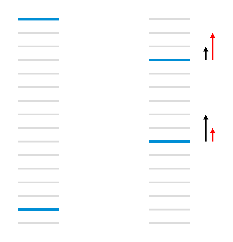
Although RankNet can be made to work quite well with the above measures by simply using the measure as a stopping criterion on a validation set, we can do better. RankNet is optimizing for (a smooth, convex approximation to) the number of pairwise errors, which is fine if that is the desired cost, but it does not match well with some other information retrieval measures. Figure 1 is a schematic depicting the problem. The idea of writing down the desired gradients directly (shown as arrows in the Figure), rather than deriving them from a cost, is one of the ideas underlying LambdaRank [4]: it allows us to bypass the difficulties introduced by the sort in most IR measures. Note that this does not mean that the gradients are not gradients of a cost. In this section, for concreteness we assume that we are designing a model to learn NDCG.
4.1 From RankNet to LambdaRank
The key observation of LambdaRank is thus that in order to train a model, we don't need the costs themselves: we only need the gradients (of the costs with respect to the model scores). The arrows ($\lambda
#39;s) mentioned above are exactly those gradients. The $\lambda#39;s for a given URL $U_1$ get contributions from all other URLs for the same query that have different labels. The $\lambda#39;s can also be interpreted as forces (which are gradients of a potential function, when the forces are conservative): if $U_2$ is more relevant than $U_1$, then $U_1$ will get a push downwards of size $|\lambda|$ (and $U_2$, an equal and opposite push upwards); if $U_2$ is less relevant than $U_1$, then $U_1$ will get a push upwards of size $|\lambda|$ (and $U_2$, an equal and opposite push downwards).Experiments have shown that modifying Eq. (3) by simply multiplying by the size of the change in NDCG ($|\Delta_{NDCG}|$) given by swapping the rank positions of $U_1$ and $U_2$ (while leaving the rank positions of all other urls unchanged) gives very good results [4]. Hence in LambdaRank we imagine that there is a utility $C$ such that[^2]
$ \lambda_{ij} = \frac{\partial C(s_i - s_j)}{\partial s_i} = \frac{-\sigma}{1 + e^{\sigma(s_i - s_j)}} |\Delta_{NDCG}|\tag{6} $
Since here we want to maximize $C$, equation (2) (for the contribution to the $k$th weight) is replaced by
$ w_k \to w_k + \eta \frac{\partial C}{\partial w_k} $
so that
$ \delta C = \frac{\partial C}{\partial w_k} \delta w_k = \eta \left( \frac{\partial C}{\partial w_k} \right)^2 > 0\tag{7} $
Thus although Information Retrieval measures, viewed as functions of the model scores, are either flat or discontinuous everywhere, the LambdaRank idea bypasses this problem by computing the gradients after the urls have been sorted by their scores. We have shown empirically that, intriguingly, such a model actually optimizes NDCG directly [12, 7]. In fact we have further shown that if you want to optimize some other information retrieval measure, such as MRR or MAP, then LambdaRank can be trivially modified to accomplish this: the only change is that $|\Delta_{NDCG}|$ above is replaced by the corresponding change in the chosen IR measure [7].
For a given pair, a $\lambda$ is computed, and the $\lambda
#39;s for $U_1$ and $U_2$ are incremented by that $\lambda$, where the sign is chosen so that $s_2 - s_1$ becomes more negative, so that $U_1$ tends to move up the list of sorted urls while $U_2$ tends to move down. Again, given more than one pair of urls, if each url $U_i$ has a score $s_i$, then for any particular pair ${U_i, U_j}$ (recall we assume that $U_i$ is more relevant than $U_j$), we separate the calculation:$ \delta s_i = \frac{\partial s_i}{\partial w_k} \delta w_k = \frac{\partial s_i}{\partial w_k} \left( -\eta \lambda \frac{\partial s_i}{\partial w_k} \right) < 0 $
$ \delta s_j = \frac{\partial s_j}{\partial w_k} \delta w_k = \frac{\partial s_j}{\partial w_k} \left( \eta \lambda \frac{\partial s_j}{\partial w_k} \right) > 0 $
Thus, every pair generates an equal and opposite $\lambda$, and for a given url, all the lambdas are incremented (from contributions from all pairs in which is it a member, where the other member of the pair has a different label). This accumulation is done for every url for a given query; when that calculation is done, the weights are adjusted based on the computed lambdas using a small (stochastic gradient) step.
[^2]: We have switched from cost to utility here since NDCG is a measure of goodness (which we want to maximize). Recall also that $S_{ij} = 1$.
4.2 LambdaRank: Empirical Optimization of NDCG (or other IR Measures)
Here we briefly describe how we showed empirically that LambdaRank directly optimizes NDCG [12, 7]. Suppose that we have trained a model and that its (learned) parameter values are $w^*_k$. We can estimate a smoothed version of the gradient empirically by fixing all weights but one (call it $w_i$), computing how the NDCG (averaged over a large number of training queries) varies, and forming the ratio
$ \frac{\delta M}{\delta w_i} = \frac{M - M^*}{w_i - w^*_i} $
where for $n$ queries
$ M \equiv \frac{1}{n} \sum_{i=1}^n NDCG(i)\tag{8} $
and where the $i$th query has NDCG equal to $NDCG(i)$. Now suppose we plot $M$ as a function of $w_i$ for each $i$. If we observe that $M$ is a maximum at $w_i = w^*_i$ for every $i$, then we know that the function has vanishing gradient at the learned values of the weights, $w = w^*$. (Of course, if we zoom in on the graph with sufficient magnification, we'll find that the curves are little step functions; we are considering the gradient at a scale at which the curves are smooth). This is necessary but not sufficient to show that the NDCG is a maximum at $w = w^*$: it could be a saddle point. We could attempt to show that the point is a maximum by showing that the Hessian is negative definite, but that is in several respects computationally challenging. However we can obtain an arbitrarily tight bound by applying a one-sided Monte Carlo test: choose sufficiently many random directions in weight space, move the weights a little along each such direction, and check that $M$ always decreases as we move away from $w^*$. Specifically, we choose directions uniformly at random by sampling from a spherical Gaussian. Let $p$ be the fraction of directions that result in $M$ increasing. Then
$ P(\text{We miss an ascent direction despite } n \text{ trials}) = (1 - p)^n $
Let's call $1 - P$ our confidence. If we require a confidence of 99% (i.e. we choose $\delta = 0.01$ and require $P \le \delta$), how large must $n$ be, in order that $p \le p_0$, where we choose $p_0 = 0.01$? We have
$ (1 - p_0)^n \le \delta \to n \ge \frac{\log \delta}{\log(1 - p_0)}\tag{9} $
which gives $n \ge 459$ (i.e. choose 459 random directions and always find that $M$ decreases along those directions; note that larger value of $p_0$ would require fewer tests). In general we have confidence at least $1 - \delta$ that $p \le p_0$ provided we perform at least $n = \frac{\log \delta}{\log(1 - p_0)}$ tests.
4.3 When are the Lambdas Actually a Gradient?
Suppose you write down some arbitrary $\lambda
#39;s. Does there necessarily exist a cost for which those $\lambda#39;s are the gradients? Are there general conditions under which such a cost exists? It's easy to write down expressions for which no function exists for which those expressions are the partial derivatives: for example, there is no $F(x, y)$ for which$ \frac{\partial F(x, y)}{\partial x} = 1, \quad \frac{\partial F(x, y)}{\partial y} = x $
It turns out that the necessary and sufficient conditions under which functions $f_1(x_1, \dots, x_n), f_2(x_1, \dots, x_n), \dots, f_n(x_1, \dots, x_n)$ are the partial derivatives of some function $F$, so that
$ \frac{\partial F}{\partial x_i} = f_i $
are that
$ \frac{\partial f_i}{\partial x_j} = \frac{\partial f_j}{\partial x_i}\tag{10} $
under the condition that the domain $\mathcal{D}$ of $F$ be open and star-shaped (in other words, if $x \in \mathcal{D}$, then all points joining $x$ with the origin are also in $\mathcal{D}$) (see for example [10]). This result is known as the Poincaré lemma. In our case, for a given pair, for any particular values for the model parameters (that is, for a particular sorting of the urls by current model scores), it is easy to write down such a cost: it is the RankNet cost multiplied by $\Delta_{NDCG}$. However the general expression depends in a complicated way on the model parameters, since the model generates the score by which the urls are sorted, and since the $\lambda
#39;s are computed after the sort.5 MART
Section Summary: MART is a boosted ensemble method that builds a scoring model as a weighted sum of regression trees, where each tree is trained via gradient descent on a general loss function to solve problems such as classification or ranking. The trees are constructed by recursively splitting data to minimize squared error around leaf means, and new trees are added to fit the negative gradients of the current loss, scaled by a small learning rate that acts as regularization. This framework is especially compatible with LambdaRank because both rely on specifying derivatives of the objective during training.
LambdaMART combines MART [8] and LambdaRank. To understand LambdaMART we first review MART. Since MART is a boosted tree model in which the output of the model is a linear combination of the outputs of a set of regression trees, we first briefly review regression trees. Suppose we are given a data set ${x_i, y_i}, i = 1, \dots, m$ where $x_i \in \mathbb{R}^d$ and the labels $y_i \in \mathbb{R}$. For a given vector $x_i$ we index its feature values by $x_{ij}, j = 1, \dots, d$. Consider first a regression stump, consisting of a root node and two leaf nodes, where directed arcs connect the root to each leaf. We think of all the data as residing on the root node, and for a given feature, we loop through all samples and find the threshold $t$ such that, if all samples with $x_{ij} \le t$ fall to the left child node, and the rest fall to the right child node, then the sum
$ S_j \equiv \sum_{i \in L} (y_i - \mu_L)^2 + \sum_{i \in R} (y_i - \mu_R)^2\tag{11} $
is minimized. Here $L (R)$ is the sets of indices of samples that fall to the left (right), and $\mu_L (\mu_R)$ is the mean of the values of the labels of the set of samples that fall to the left (right). (The dependence on $j$ in the sum appears in $L, R$ and in $\mu_L, \mu_R$). $S_j$ is then computed for all choices of feature $j$ and all choices of threshold for that feature, and the split (the choice of a particular feature $j$ and threshold $t$) is chosen that gives the overall minimal $S_j$. That split is then attached to the root node. For the two leaf nodes of our stump, a value $\gamma_l, l = 1, 2$ is computed, which is just the mean of the $y
#39;s of the samples that fall there. In a general regression tree, this process is continued $L - 1$ times to form a tree with $L$ leaves[^3].[^3]: We are overloading notation (the meaning of $L$) in just this paragraph.
MART is a class of boosting algorithms that may be viewed as performing gradient descent in function space, using regression trees. The final model again maps an input feature vector $x \in \mathbb{R}^d$ to a score $F(x) \in \mathbb{R}$. MART is a class of algorithms, rather than a single algorithm, because it can be trained to minimize general costs (to solve, for example, classification, regression or ranking problems). Note, however, that the underlying model upon which MART is built is the least squares regression tree, whatever problem MART is solving. MART's output $F(x)$ can be written as
$ F_N(x) = \sum_{i=1}^N \alpha_i f_i(x) $
where each $f_i(x) \in \mathbb{R}$ is a function modeled by a single regression tree and the $\alpha_i \in \mathbb{R}$ is the weight associated with the $i$th regression tree. Both the $f_i$ and the $\alpha_i$ are learned during training. A given tree $f_i$ maps a given $x$ to a real value by passing $x$ down the tree, where the path (left or right) at a given node in the tree is determined by the value of a particular feature $x_j, j = 1, \dots, d$ and where the output of the tree is taken to be a fixed value associated with each leaf, $\gamma_{kn}, k = 1, \dots, L, n = 1, \dots, N$, where $L$ is the number of leaves and $N$ the number of trees. Given training and validation sets, the user-chosen parameters of the training algorithm are $N$, a fixed learning rate $\eta$ (that multiplies every $\gamma_{kn}$ for every tree), and $L$. (One could also choose different $L$ for different trees). The $\gamma_{kn}$ are also learned during training.
Given that, say, $n$ trees have been trained, how should the next tree be trained? MART uses gradient descent to decrease the loss: specifically, the next regression tree models the $m$ derivatives of the cost with respect to the current model score evaluated at each training point: $\frac{\partial C}{\partial F_n}(x_i), i = 1, \dots, m$. Thus:
$ \delta C \approx \frac{\partial C(F_n)}{\partial F_n} \delta F\tag{12} $
and so $\delta C < 0$ if we take $\delta F = -\eta \frac{\partial C}{\partial F_n}$. Thus each tree models the gradient of the cost with respect to the model score, and the new tree is added to the ensemble with a step size $\eta \gamma_{kn}$. The step sizes $\gamma_{kn}$ can be computed exactly in some cases, or using Newton's approximation in others. The role of $\eta$ as an overall learning rate is similar to that in other stochastic gradient descent algorithms: taking a step that is smaller than the optimal step size (i.e. the step size that maximally reduces the cost) acts as a form of regularization for the model that can significantly improve test accuracy.
Clearly, since MART models derivatives, and since LambdaRank works by specifying the derivatives at any point during training, the two algorithms are well matched: LambdaMART is the marriage of the two [11].
To understand MART, let's next examine how it works in detail, for perhaps the simplest supervised learning task: binary classification.
6 MART for Two Class Classification
Section Summary: MART adapts gradient-boosted regression trees to binary classification by treating the problem as logistic regression with ±1 labels and a cross-entropy loss. At each iteration it computes per-example gradients that serve as targets for a regression tree, then uses a single Newton-Raphson step to choose the additive adjustment that most reduces the loss in every leaf. The resulting procedure is unchanged by the choice of sigmoid scaling and can be re-weighted to handle severely unbalanced data.
We follow [8], although we give a somewhat different emphasis here; in particular, we allow a general sigmoid parameter $\sigma$ (although it turns out that choice of $\sigma$ does not make affect the model, it's instructive to see why).
We choose labels $y_i \in {\pm 1}$ (this has the advantage that $y_i^2 = 1$, which will be used later). The model score for sample $x \in \mathbb{R}^n$ is denoted $F(x)$. To keep notation brief, denote the modeled conditional probabilities by $P_+ \equiv P(y = 1|x)$ and $P_- \equiv P(y = -1|x)$, and define indicators $I_+(x_i) = 1$ if $y_i = 1, 0$ otherwise, and $I_-(x_i) = 1$ if $y_i = -1, 0$ otherwise. We use the cross-entropy loss function (the negative binomial log-likelihood):
$ L(y, F) = -I_+ \log P_+ - I_- \log P_- $
(Note the similarity to the RankNet loss). Logistic regression models the log odds. So if $F_N(x)$ is the model output, we choose (the factor of $\frac{1}{2}$ here is included to match [8]):
$ F_N(x) = \frac{1}{2} \log \left( \frac{P_+}{P_-} \right)\tag{13} $
or
$ P_+ = \frac{1}{1 + e^{-2\sigma F_N(x)}}, \quad P_- = 1 - P_+ = \frac{1}{1 + e^{2\sigma F_N(x)}} $
which gives
$ L(y, F_N) = \log(1 + e^{-2y\sigma F_N})\tag{14} $
The gradients of the cost with respect to the model scores (called pseudoresponses in [8]) are:
$ \bar{y}i = -\left[ \frac{\partial L(y_i, F(x_i))}{\partial F(x_i)} \right]{F(x)=F_{m-1}(x)} = \frac{2y_i\sigma}{1 + e^{2y_i\sigma F_{m-1}(x)}} $
These are the exact analogs of the Lambda gradients in LambdaRank (and in fact are the gradients in LambdaMART). They are the values that the regression tree is modeling. Denoting the set of samples that land in the $j$th leaf node of the $m$th tree by $R_{jm}$, we want to find an approximately optimal step for each leaf, that is, the values that minimize the loss:
$ \gamma_{jm} = \text{arg}\min_\gamma \sum_{x_i \in R_{jm}} \log(1 + e^{-2y_i\sigma(F_{m-1}(x_i) + \gamma)}) \equiv \text{arg}\min_\gamma g(\gamma) $
The Newton approximation is used to find $\gamma$: for a function $g(\gamma)$, a Newton-Raphson step towards the extremum of $g$ is
$ \gamma_{n+1} = \gamma_n - \frac{g'(\gamma_n)}{g''(\gamma_n)} $
Here we start from $\gamma = 0$ and take just one step. Again let's simplify the expressions by collapsing notation: define $S_i(\gamma) \equiv 1 + e^{-2v_i} \equiv 1 + e^{-2y_i\sigma(F_{m-1}(x) + \gamma)}$. We want to compute
$ \text{arg}\min_\gamma g(\gamma) \equiv \text{arg}\min_\gamma \sum_{x_i \in R_{jm}} \log S_i(\gamma) $
Now
$ g' = \sum_{x_i \in R_{jm}} \frac{1}{S_i} (-2y_i\sigma e^{-2v_i}) $
$ g'' = \sum_{x_i \in R_{jm}} \frac{-1}{S_i^2} (-2y_i\sigma e^{-2v_i})^2 - \frac{2y_i\sigma}{S_i} (-2y_i\sigma)e^{-2v_i} = \sum_{x_i \in R_{jm}} \frac{4}{S_i^2} y_i^2 \sigma^2 e^{-2v_i} $
But
$ \bar{y}i \equiv \frac{2y_i\sigma}{1 + e^{2y_iF}} \Rightarrow g' = \sum{x_i \in R_{jm}} -\frac{2y_i\sigma}{e^{2v_i}S_i} = \sum_{x_i \in R_{jm}} -\bar{y}_i $
Also
$ g'' = \sum_{x_i \in R_{jm}} \frac{4y_i^2\sigma^2}{(1 + e^{2v_i})^2} e^{2v_i} $
Since $y_i^2 = 1$ we have
$ |\bar{y}_i| = \frac{2\sigma}{1 + e^{2v_i}} $
so
$ |\bar{y}_i| (2\sigma - |\bar{y}_i|) = \frac{4\sigma^2 e^{2v_i}}{(1 + e^{2v_i})^2} $
giving simply
$ \gamma_{jm} = -\frac{g'}{g''} = \frac{\sum_{x_i \in R_{jm}} \bar{y}i}{\sum{x_i \in R_{jm}} |\bar{y}_i|(2\sigma - |\bar{y}_i|)} $
(This corresponds to Algorithm 5 in [8]). Note that this step combines both the estimate of the gradient (the numerator) and the usual gradient descent step size (in this case, $1/g''$). To include a learning rate $r$, we just multiply each leaf value $\gamma_{jm}$ by $r$.
It's interesting that for this algorithm, the value of $\sigma$ makes no difference. The Newton step $\gamma_{jm}$ is proportional to $1/\sigma$. Since $F_m(x) = F_{m-1}(x) + \gamma$, and since $F$ appears with an overall factor of $\sigma$ in the loss, the $\sigma
#39;s just cancel in the loss function.6.1 Extending to Unbalanced Data Sets
For completeness we include a discussion on how to extend the algorithm to cases where the data is very unbalanced (e.g. far more positive examples than negative).
If $n_+ (n_-)$ is the total number of positive (negative) examples, for unbalanced data a useful way to count errors is:
$ \text{error rate} = \frac{\text{number false positives}}{2n_-} + \frac{\text{number false negatives}}{2n_+} $
The factor of two in the denominator is just to scale so that the maximum error rate is one. We still use logistic regression (model the log odds) but instead use the balanced loss:
$ L_B(y, F) = -\frac{I_+}{n_+} \log P_+ - \frac{I_-}{n_-} \log P_- = \left( \frac{I_+}{n_+} + \frac{I_-}{n_-} \right) \log(1 + e^{-2y\sigma F}) $
The equations are similar to before. The gradients $\bar{y}_i$ are replaced by
$ \bar{z}i = -\left[ \frac{\partial L_B(y_i, F(x_i))}{\partial F(x_i)} \right]{F(x)=F_{m-1}(x)} = \bar{y}i \left( \frac{I+}{n_+} + \frac{I_-}{n_-} \right) $
and the Newton step becomes
$ \gamma_{jm}^B = -\frac{g'}{g''} = \frac{\sum_{x_i \in R_{jm}} \bar{y}i \left( \frac{I+}{n_+} + \frac{I_-}{n_-} \right)}{\sum_{x_i \in R_{jm}} |\bar{y}i|(2\sigma - |\bar{y}i|) \left( \frac{I+}{n+} + \frac{I_-}{n_-} \right)}\tag{15} $
(Note that this is not the same as the previous Newton step with $\bar{y}_i$ replaced by $\bar{z}_i$.)
7 LambdaMART
Section Summary: LambdaMART combines gradient boosting via regression trees, or MART, with the LambdaRank approach to directly optimize ranking metrics such as NDCG. It defines per-item gradients as pairwise lambdas that reflect both preference errors and utility changes from swaps, then builds each tree on the full dataset using least squares splits and Newton-step leaf values derived from the first and second derivatives of an implicit cost function. The resulting procedure supports an optional base model, processes all training data at once when choosing splits, and can outperform query-by-query methods like LambdaRank in overall utility gains.
To implement LambdaMART we just use MART, specifying appropriate gradients and the Newton step. The gradients $\bar{y}i$ are easy: they are just the $\lambda_i$. As always in MART, least squares is used to compute the splits. In LambdaMART, each tree models the $\lambda_i$ for the entire dataset (not just for a single query). To compute the Newton step, we collect some results from above: for any given pair of urls $U_i$ and $U_j$ such that $U_i \triangleright U_j$, then after the urls have been sorted by score, the $\lambda{ij}
#39;s are defined as (see Eq. (4))$ \lambda_{ij} = \frac{-\sigma|\Delta Z_{ij}|}{1 + e^{\sigma(s_i - s_j)}}, $
where we write the utility difference generated by swapping the rank positions of $U_i$ and $U_j$ as $Z_{ij}$ (for example, $Z$ might be NDCG). We also have
$ \lambda_i = \sum_{j:{i,j} \in I} \lambda_{ij} - \sum_{j:{j,i} \in I} \lambda_{ij} $
To simplify notation, let's denote the above sum operation as follows:
$ \sum_{{i,j} \in I} \lambda_{ij} \equiv \sum_{j:{i,j} \in I} \lambda_{ij} - \sum_{j:{j,i} \in I} \lambda_{ij} $
Thus, for any given state of the model (i.e. for any particular set of scores), and for a particular url $U_i$, we can write down a utility function for which $\lambda_i$ is the derivative of that utility[^4]
$ C = \sum_{{i,j} \in I} |\Delta Z_{ij}| \log(1 + e^{-\sigma(s_i - s_j)}) $
so that
$ \frac{\partial C}{\partial s_i} = \sum_{{i,j} \in I} \frac{-\sigma|\Delta Z_{ij}|}{1 + e^{\sigma(s_i - s_j)}} \equiv \sum_{{i,j} \in I} -\sigma|\Delta Z_{ij}| \rho_{ij} $
where we've defined
$ \rho_{ij} \equiv \frac{1}{1 + e^{\sigma(s_i - s_j)}} = \frac{-\lambda_{ij}}{\sigma|Z_{ij}|} $
Then
$ \frac{\partial^2 C}{\partial s_i^2} = \sum_{{i,j} \in I} \sigma^2 |\Delta Z_{ij}| \rho_{ij}(1 - \rho_{ij}) $
[^4]: We switch back to utilities here but use C to match previous notation.
(using $\frac{e^x}{(1+e^x)^2} = (1 - \frac{1}{1+e^x}) \frac{1}{1+e^x}$) and the Newton step size for the $k$th leaf of the $m$th tree is
$ \gamma_{km} = \frac{\sum_{x_i \in R_{km}} \frac{\partial C}{\partial s_i}}{\sum_{x_i \in R_{km}} \frac{\partial^2 C}{\partial s_i^2}} = \frac{-\sum_{x_i \in R_{km}} \sum_{{i,j} \in I} |\Delta Z_{ij}| \rho_{ij}}{\sum_{x_i \in R_{km}} \sum_{{i,j} \in I} |\Delta Z_{ij}| \sigma \rho_{ij}(1 - \rho_{ij})} $
(note the change in sign since here we are maximizing). In an implementation it is convenient to simply compute $\rho_{ij}$ for each sample $x_i$; then computing $\gamma_{km}$ for any particular leaf node just involves performing the sums and dividing. Note that, just as for logistic regression, for a given learning rate $\eta$, the choice of $\sigma$ will make no difference to the training, since the $\gamma_{km}
#39;s scale as $1/\sigma$, the model score is always incremented by $\eta \gamma_{km}$, and the scores always appear multiplied by $\sigma$.We summarize the LambdaMART algorithm schematically below. As pointed out in [11], one can easily perform model adaptation by starting with the scores given by an initial base model.
Algorithm: LambdaMART
set number of trees N, number of training samples m, number of leaves per tree L, learning rate $\eta$
for $i = 0$ to $m$ do
  $F_0(x_i) = \text{BaseModel}(x_i)$ //If BaseModel is empty, set $F_0(x_i) = 0$
end for
for $k = 1$ to $N$ do
  for $i = 0$ to $m$ do
    $y_i = \lambda_i$
    $w_i = \frac{\partial y_i}{\partial F_{k-1}(x_i)}$
  end for
  $\{R_{lk}\}_{l=1}^L$ // Create $L$ leaf tree on $\{x_i, y_i\}_{i=1}^m$
  $\gamma_{lk} = \frac{\sum_{x_i \in R_{lk}} y_i}{\sum_{x_i \in R_{lk}} w_i}$ // Assign leaf values based on Newton step.
  $F_k(x_i) = F_{k-1}(x_i) + \eta \sum_l \gamma_{lk} I(x_i \in R_{lk})$ // Take step with learning rate $\eta$.
end for
Finally it's useful to compare how LambdaRank and LambdaMART update their parameters. LambdaRank updates all the weights after each query is examined. The decisions (splits at the nodes) in LambdaMART, on the other hand, are computed using all the data that falls to that node, and so LambdaMART updates only a few parameters at a time (namely, the split values for the current leaf nodes), but using all the data (since every $x_i$ lands in some leaf). This means in particular that LambdaMART is able to choose splits and leaf values that may decrease the utility for some queries, as long as the overall utility increases.
7.1 A Final Note: How to Optimally Combine Rankers
We end with the following note: [11] contains a relatively simple method for linearly combining two rankers such that out of all possible linear combinations, the resulting ranker gets the highest possible NDCG (in fact this can be done for any IR measure). The key trick is to note that if $s^1_i$ are the outputs of the first ranker (for a given query), and $s^2_i$ those of the second, then the output of the combined ranker can be written $\alpha s^1_i + (1 - \alpha)s^2_i$, and as $\alpha$ sweeps through its values (say, from 0 to 1), then the NDCG will only change a finite number of times. We can simply (and quite efficiently) keep track of each change and keep the $\alpha$ that gives the best combined NDCG. However it should also be noted that one can achieve a similar goal (without the guarantee of optimality, however) by simply training a linear (or nonlinear) LambdaRank model using the previous model scores as inputs. This usually gives equally good results and is easier to extend to several models.
Acknowledgements The work described here has been influenced by many people. Apart from the co-authors listed in the references, I'd like to additionally thank Qiang Wu, Krysta Svore, Ofer Dekel, Pinar Donmez, Yisong Yue, and Galen Andrew.
References
Section Summary: This section compiles a numbered list of academic papers, technical reports, and books cited in support of the main text. Most entries focus on machine learning techniques for ranking and information retrieval, such as neural networks, gradient-based optimization, and evaluation measures, primarily from conferences and journals in the 2000s, with a few foundational references from earlier decades.
[1] E.B. Baum and F. Wilczek. Supervised Learning of Probability Distributions by Neural Networks. Neural Information Processing Systems, American Institute of Physics, 1988.
[2] C.J.C. Burges, T. Shaked, E. Renshaw, A. Lazier, M. Deeds, N. Hamilton and G. Hullender. Learning to Rank using Gradient Descent. Proceedings of the Twenty Second International Conference on Machine Learning, 2005.
[3] C.J.C. Burges. Ranking as Learning Structured Outputs. Neural Information Processing Systems workshop on Learning to Rank, Eds. S. Agerwal, C. Cortes and R. Herbrich, 2005.
[4] C.J.C. Burges, R. Ragno and Q.V. Le. Learning to Rank with Non-Smooth Cost Functions. Advances in Neural Information Processing Systems, 2006.
[5] O. Chapelle, Y. Chang and T-Y Liu. The Yahoo! Learning to Rank Challenge. http://learningtorankchallenge.yahoo.com, 2010.
[6] O. Chapelle, D. Metzler, Y. Zhang and P. Grinspan. Expected Reciprocal Rank for Graded Relevance Measures. International Conference on Information and Knowledge Management (CIKM), 2009.
[7] P. Donmez, K. Svore and C.J.C. Burges. On the Local Optimality of LambdaRank. Special Interest Group on Information Retrieval (SIGIR), 2009.
[8] J.H. Friedman. Greedy function approximation: A gradient boosting machine. Technical Report, IMS Reitz Lecture, Stanford, 1999; see also Annals of Statistics, 2001.
[9] K. Jarvelin and J. Kekalainen. IR evaluation methods for retrieving highly relevant documents. Special Interest Group on Information Retrieval (SIGIR), 2000.
[10] M. Spivak. Calculus on Manifolds. Addison-Wesley, 1965.
[11] Q. Wu, C.J.C. Burges, K. Svore and J. Gao. Adapting Boosting for Information Retrieval Measures. Journal of Information Retrieval, 2007.
[12] Y. Yue and C.J.C. Burges. , On Using Simultaneous Perturbation Stochastic Approximation for Learning to Rank, and the Empirical Optimality of LambdaRank. Microsoft Research Technical Report MSR-TR-2007-115, 2007.