
Replicable Conformal Prediction
Marios Papamichalis $^{}$
$^{}$ Human Nature Lab, Yale University, New Haven, CT 06511, USA. [email protected]
Regina Ruane $^{\dagger}$
$^{\dagger}$ Department of Statistics and Data Science, The Wharton School, University of Pennsylvania, Philadelphia, PA, USA. [email protected]
Theofanis Papamichalis $^{\ddagger}$
$^{\ddagger}$ Department of Economics, Yale University, New Haven, CT, USA. [email protected]
Abstract
Two analysts who calibrate a conformal predictor on independent samples deploy different set-valued classifiers with probability one, because the calibrated threshold is an order statistic of continuous scores. We ask when the identical classifier can be deployed, and at what cost. Exact agreement is impossible: a procedure that returns one fixed output with high probability cannot be uniformly valid, and with a shared seed an exactly replicable procedure must ignore its data. Rounding the threshold upward on a shared-seed random grid (replicable calibration, RECAL) makes the deployed classifier identical across analysts with probability at least $1-\rho$, preserves marginal coverage, keeps training-conditional coverage within $\varepsilon$ of target, and needs $O(\kappa^{2}\alpha(1-\alpha)/(\varepsilon^{2}\rho^{2}))$ calibration points at miscoverage level $\alpha$, where $\kappa$ bounds the local score-density ratio. Lower bounds with explicit constants show the sample cost and a coverage inflation of order $\sqrt{\alpha(1-\alpha)/n}/\rho$ at calibration size $n$ are unavoidable for any threshold calibrator; a consistent plug-in removes the factor $\kappa^{2}$ asymptotically. Without any seed, a deterministic grid confines all analysts to two adjacent classifiers, optimally. Selecting the most favorable of $M$ recalibrations changes a RECAL classifier with probability at most $(M-1)\rho$; the same selection silently undercovers standard split conformal. Experiments on real ImageNet outputs, a four-hospital site split, four language-model families, and synthetic testbeds match the theory, including the predicted $(\varepsilon\rho)^{-2}$ sample frontier.
Executive Summary: Standard split conformal prediction turns a fixed model into a set-valued classifier by calibrating a threshold on held-out scores. Because that threshold is an order statistic of continuous scores, two analysts who calibrate independently on i.i.d. samples almost surely deploy different classifiers. This instability is invisible to ordinary coverage checks yet creates practical difficulties: hospitals or regulators cannot certify a single frozen artifact, serving systems cannot safely cache predictions, and an adversary who redraws the calibration set multiple times and keeps the most favorable draw can produce undercovering sets that still pass support audits. The instability is therefore both a reproducibility failure and a selective-inference vulnerability at deployment time.
The paper asks when two independent calibrations can be made to return exactly the same classifier with high probability while retaining the finite-sample coverage guarantee, what sample and set-size cost this requires, and whether the resulting procedure protects against selective recalibration.
The authors first prove impossibility results for exact replication, then introduce ReCal: a shared-seed procedure that rounds the usual conformal quantile upward onto a random grid whose offset is drawn once from a shared uniform random variable. Analysis relies on the exact Beta law of realized coverage, a local margin condition on the score density near the target quantile, and explicit finite-sample tail bounds. Lower bounds are derived by reduction to a replicable-coin problem on a carefully chosen hard family of distributions. The procedure is evaluated on synthetic ImageNet-scale data, real ImageNet logits, four language-model families, a four-hospital clinical split, and controlled small-data regimes, with replication metrics (identity, pointwise agreement, churn mass, and list membership) reported alongside coverage and set size.
Exact identity is impossible for any uniformly valid procedure that returns a single fixed classifier with probability greater than 1−min{α,1−α}; with a shared seed, exact replicability forces the output law to be data-oblivious. ReCal achieves ρ-replicability, preserves marginal coverage ≥1−α, and keeps training-conditional coverage within ε of target using n = O(κ² α(1−α)/(ε² ρ²)) calibration points. Matching lower bounds (with explicit constants) show that any threshold-based replicable calibrator must pay a sample cost of the same order and must inflate coverage by Ω(√[α(1−α)/n]/ρ). Selective recalibration of M independent runs changes the deployed classifier with probability at most min{1,(M−1)ρ} and degrades expected coverage by at most the same amount. Without a shared seed, deterministic-grid rounding confines all analysts to a common two-element list of adjacent thresholds. Experiments confirm the predicted (ερ)⁻² sample frontier, the geometry of churn concentration, and the selection bound; identity rates reach the design targets once a modest safety factor on the margin constant is used.
Replicable calibration converts an unverifiable and exploitable source of variability into a checkable property of the deployed artifact. It therefore supports auditing, caching, version control, and joint deployment across independent parties, while simultaneously bounding the coverage loss that selective recalibration can inflict. The set-size premium is unavoidable for any replicable threshold procedure and is paid in score mass; on long-tailed vocabularies the translation into set size can be large unless rank regularization is applied. The procedure works unchanged for any nested family (APS, RAPS, conformal risk control, conformal LM stopping) that calibrates a single scalar.
For settings that require a single verifiable classifier, adopt ReCal with a pre-registered shared seed and κ̂ = 1.5 (or a data-driven pilot when sample size permits). When shared randomness is unavailable, use the deterministic-grid two-list variant and verify that every analyst’s threshold lies in the certified adjacent pair. For long-tailed scores, combine ReCal with rank regularization. When further reduction of the finite-sample κ² factor is needed, run the asymptotically exact plug-in pilot. Before production use at very small calibration sizes, conduct a short pilot to confirm that the realized identity rate meets the design target.
The sharpest rates require a local margin condition; without it the distribution-free binary-search fallback remains valid but pays an extra logarithmic factor. The analysis is for threshold calibrators on nested families; full conformal and arbitrary refitted maps are outside its scope. Real-image and clinical experiments use modest sample sizes or cross-validated scores; frozen production-scale deployment remains future work. The theory and all reported experiments are consistent with the stated constants and rates.
1. Introduction
Section Summary: Conformal prediction produces classifiers with reliable coverage guarantees by calibrating a threshold on held-out data, but independent calibrations on different samples almost always yield different output sets, creating instability that can be exploited through selective recalibration and undermining auditability or reproducibility. The paper introduces replicable calibration methods that use a shared random seed to force two independent runs to agree on the exact same classifier with high probability, while preserving the original validity guarantees at a modest increase in sample size or prediction-set size. It also proves fundamental limits showing when exact agreement is impossible without shared randomness or under strong uniformity requirements.
Conformal prediction converts a trained model into a set-valued classifier with a finite-sample coverage guarantee ([1, 2, 3]): a threshold $\widetilde{\tau}$ is calibrated on $n$ held-out points, the classifier $\mathcal{C}(x)={y:s(x, y)\le \widetilde{\tau}}$ is deployed, and the probability that the true label is covered is at least $1-\alpha$. In deployment the calibrated classifier is an artifact: hashed, cached, versioned, audited. Three examples motivate this paper: two hospitals validate one frozen diagnostic model on their own held-out data before a joint deployment; a regulator re-runs a vendor's calibration during an audit; a serving system caches conformal answer sets for language-model decoding ([4]). In each case the question is whether two independent calibrations produce the identical classifier, a stronger event than achieving similar coverage.
With standard split conformal they never do. The calibrated threshold is an order statistic of continuously distributed scores, so two independent calibrations agree with probability zero (Proposition 3), and realized coverage fluctuates across calibration draws according to an exact Beta law ([5]). The instability is exploitable: a party that redraws its calibration set $M$ times and keeps the most favorable draw deploys sets that undercover by an amount on the order of $\sqrt{\log M}$ times the coverage standard deviation (Corollary 9), while the artifact passes any support check (Section 8, Figure 1 b). A selective-inference failure at the deployment layer ([6, 7]): candidate-wise validity does not survive selection ([8]); replicability restores selection robustness (Corollary 9). Cross-sample instability is documented at benchmark scale ([9]); for prediction sets, built to be audited, it undermines that function.
A separate line of work formalizes agreement across independent samples. An algorithm is $\rho$-replicable if two runs on independent samples that share an internal random seed return the identical output with probability at least $1-\rho$ ([10]); the theory covers costs, list relaxations, and connections to privacy and stability ([11, 12, 13, 14]). To our knowledge the framework has not previously been applied to conformal prediction or distribution-free uncertainty quantification; this paper does so and characterizes the achievable trade-offs for conformal calibration.
Questions.
First, can any procedure return one fixed classifier with high probability and remain valid for every distribution? Second, we determine which relaxed agreements are achievable, at what sample and set-size cost, and whether that cost is necessary. Third, we quantify what replicable calibration guarantees against selective recalibration.
Answers.
Exact agreement is impossible in a strong sense: any procedure that outputs one fixed classifier with probability $1-\delta$ and is uniformly valid to within $\varepsilon$ cannot exist when $\varepsilon+\delta<\min{\alpha, 1-\alpha}$; with a shared seed, exact replicability forces the output law to be the same under every distribution, so the deployed sets are uninformative (Theorem 4). Rounding the threshold upward on a random grid whose offset is generated from one shared seed ($\textsc{ReCal}$; Algorithm 1) makes the deployed classifier $\rho$-replicable, preserves the marginal guarantee, and keeps a two-sided training-conditional band, at sample complexity $O(\kappa^{2}\alpha(1-\alpha)/(\varepsilon^{2}\rho^{2}))$ under a local margin condition (Theorem 6). A direct argument shows $n\ge\tfrac{9}{16384}, \alpha(1-\alpha)/(\varepsilon^{2}\rho^{2})$ is necessary for any threshold calibrator (Theorem 13), and the same machinery bounds the set-size cost: any replicable threshold calibrator inflates coverage by $\Omega(\sqrt{\alpha(1-\alpha)/n}/\rho)$, which $\textsc{ReCal}$ attains up to $\kappa^{2}$ (Corollary 14); a consistent pilot removes the prior constant and the $\kappa^{2}$ asymptotically (Proposition 12). Without a shared seed, single-answer replication is impossible below failure probability $1/2$; a deterministic grid places every analyst, with probability $1-\delta$, in a common two-element list of adjacent classifiers at rate $O(\kappa^{2}\log(1/\delta)/\varepsilon^{2})$, optimal within the margin class (Theorem 16).
What exact identity provides, and what it costs.
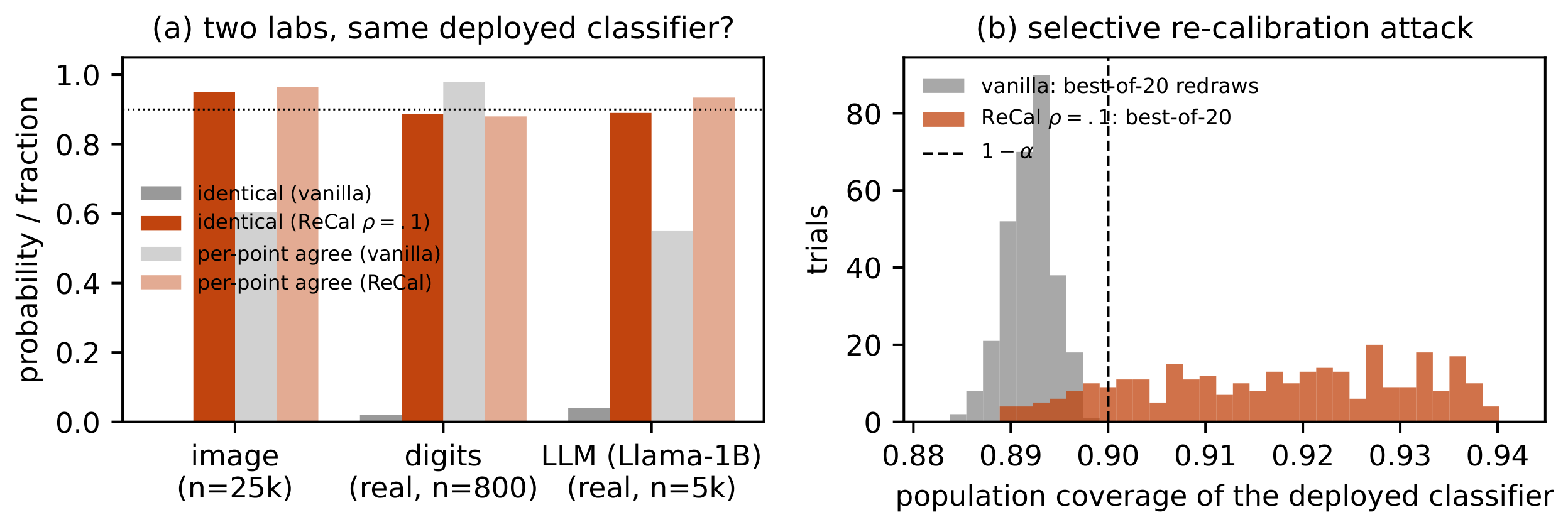
Identity is the relevant event wherever artifacts are hashed, cached, or certified, and it bounds selection: with a pre-registered seed, $M$ calibration redraws yield a second distinct classifier with probability at most $\min{1, (M-1)\rho}$, and expected coverage degrades by at most the same amount (Corollary 9); continuous stability notions such as one-point stability ([15]) do not provide this. Identity has a cost beyond set size: $\textsc{ReCal}$ concentrates disagreement into rare full-grid-cell events, so on small-sample real data pointwise agreement can decrease while identity rises from $0$ to $0.9$; we therefore report a full spectrum of replication metrics (Definition 1).
Contributions.
(C1) Impossibility theory: obliviousness of exact replication, necessity of shared randomness, and a seedless two-element-list frontier with matching optimality (Theorem 4 and Theorem 16). (C2) $\textsc{ReCal}$, a replicable split-conformal calibrator with preserved validity and explicit constants, with corollaries for unequal calibration sizes, selective recalibration, and robustness to score and population mismatch, and a pilot procedure with confidence bands whose single prior input ($\hat\kappa\ge\kappa$) is identified, stress-tested, and asymptotically unnecessary (Theorem 6, Corollary 7, Corollary 8, and Corollary 9, Corollary 25 in Appendix B, Proposition 10 and Proposition 12). (C3) Lower bounds with the $\alpha(1-\alpha)$ dependence, proved directly with explicit constants and attained up to the factor $\kappa^{2}$, for the sample size and for the set-size cost, with a lemma localizing where the cost surfaces (Theorem 13, Corollary 14, Lemma 15). (C4) An instrumented version of the standard conformal evaluation ([16, 17]) adding replication metrics (a set-valued, calibration-resampling analogue of the churn analysis of [9]), applied to a synthetic image-scale testbed, a real small-data task, and next-token logits from four language-model families ($50$ k– $152$ k vocabularies), with direct measurements of the frontier and the selection attack; all synthetic results regenerate deterministically on one CPU core.
2. Related work
Section Summary: Research on replicability has linked the concept to differential privacy, global stability, and related lower bounds, while producing algorithms for tasks such as statistical queries, bandits, and quantiles, often incurring logarithmic overhead. Work on conformal prediction has established calibration methods, risk-control extensions, and ways to manage variability or privacy, yet typically focuses on single-run guarantees rather than consistent outputs across independent data samples. The section positions the present paper as extending these lines by adding set-level identity semantics, tighter distribution-free bounds, and theory for list size and obliviousness while treating earlier quantile constructions as a fallback.
Replicability. [10] introduced $\rho$-replicability with replicable statistical queries and a coin-problem lower bound of $\Omega(1/\rho^{2})$ at fixed tolerance; [11] connected replicability, differential privacy, and perfect generalization (with an inherent quadratic overhead in one direction); [13, 18] tie replicability to global stability and Borsuk–Ulam obstructions underlying list-size lower bounds; [12] formalize list/certificate replicability; [14] resolve the $N$-coin problem via isoperimetry; replicable bandits, RL, and testing followed ([19, 20, 21]). Closest algorithmically is the replicable quantile of [22], Thm. B.6 ($\widetilde{O}(\log^{2}R/(\alpha^{2}\rho^{2}))$ over an $R$-point grid via statistical-query (SQ) binary search); relative to it we contribute the conformal semantics (set-level identity with the finite-sample guarantee kept, two-sided coverage bands, unequal- $n$ analysts), constants via the exact Beta law (no $\log^{2}R$; Remark 11), the coverage-metric lower bound, and the obliviousness/list theory; their construction is our distribution-free fallback (Proposition 29).
Conformal prediction. Foundations and training-conditional behavior: [1, 2, 5, 23]; APS/RAPS define the scores and evaluation we instrument ([16, 17]); nested families ([24]) coincide with our output class; conformal risk control (CRC) and conformal-LM stopping ([25, 4]) calibrate one scalar, so $\textsc{ReCal}$ applies unchanged (we instantiate a risk-controlled variant in Section 8). One-point stability ([15]) and e-value derandomization ([26]) are within-run notions, orthogonal to cross-sample identity. [27] ask when one calibration set may be reused across predictions; we ask when two different sets yield one classifier. [28], App. C make a single run deterministic via input-hash jitter; we adopt the device for tie-breaking (Remark 2) and show it leaves cross-sample identity at zero; post-selection inference conditions on the selection ([6, 8, 7]), while Corollary 9 makes the selected object nearly deterministic, a complementary route (Table 1). Private prediction sets ([29]) privatize the same quantile; the generic DP-to-replicability conversion ([11]) costs quadratic overhead and a shared seed anyway. Prediction churn and multiplicity are documented deployment problems ([30, 31, 9]); replicable calibration yields one verifiable classifier.
3. Preliminaries: calibration and replication metrics
Section Summary: Split conformal prediction uses a fixed scoring function on held-out data to set a threshold that guarantees marginal coverage at level 1-α, with the exact coverage distribution following a Beta law when scores are continuous. Replicability requires that two independent runs on data from the same distribution produce identical outputs with high probability, or at least land in a small list of possible outputs, and this property is preserved by any deterministic post-processing of the threshold. The section introduces a spectrum of metrics to assess replication quality—from exact identity of the resulting prediction sets to average pointwise agreement and churn—and shows that ordinary split conformal fails to replicate because independent calibrations almost surely yield different thresholds and therefore different sets.
Split conformal. $(X_i, Y_i)\overset{\text{iid}}{\sim}P$ on $\mathcal{X}\times \mathcal{Y}$; $s: \mathcal{X}\times \mathcal{Y}\to \mathbb{R}$ is a fixed measurable score (a frozen artifact); $S_i=s(X_i, Y_i)$ has continuous law $F$ (Remark 2); $q=F^{-1}(1-\alpha)$. With $k=\lceil(1-\alpha)(n+1)\rceil$ and $\alpha\ge1/(n+1)$, the threshold is $\widetilde{\tau}n=S{(k)}$, the deployed classifier is $\mathcal{C}\tau(\cdot)={y:s(\cdot, y)\le\tau}$ at $\tau= \widetilde{\tau}n$, and $\mathbb{P}(Y{n+1}\in \mathcal{C}{\widetilde{\tau}n}(X{n+1}))\ge1-\alpha$. For continuous $F$, $F(\widetilde{\tau}_n)\overset{d}{=}\mathrm{Beta}(k, n{+}1{-}k)$, the exact law of realized coverage ([5]).
Replicability. A calibrator $\mathcal{A}$ maps $(\mathcal{D}, r)$ to an output, $r$ a shared random string. $\mathcal{A}$ is $\rho$-replicable over a class $\mathcal{P}$ if $\mathbb{P}_{\mathcal{D}, \mathcal{D}'\sim P^{\otimes n}, r}[\mathcal{A}(\mathcal{D};r)\neq \mathcal{A}(\mathcal{D}';r)]\le\rho$ for all $P\in \mathcal{P}$ ([10]); it is $(\ell, \delta)$-list replicable if for every $P$ there is $\mathcal{L}(P)$, $| \mathcal{L}(P)|\le\ell$, with $\mathbb{P}[\mathcal{A}(\mathcal{D};r)\in \mathcal{L}(P)]\ge1-\delta$ ([12]). Both are preserved under deterministic post-processing. For threshold calibrators, identical $\tau$ gives identical set maps at every test input.
########## {caption="Definition 1: Replication spectrum"}
For two runs producing set maps $\mathcal{C}, \mathcal{C}'$ we track four criteria: (i) identity $\mathbb{P}[\mathcal{C}\equiv \mathcal{C}']$; (ii) pointwise agreement $\mathbb{E}{X}, \mathbb{P}[\mathcal{C}(X)= \mathcal{C}'(X)]$; (iii) churn mass $\mathbb{E}{X}, | \mathcal{C}(X), \triangle, \mathcal{C}'(X)|$, also reported conditionally on $\mathcal{C}(X)\neq \mathcal{C}'(X)$; (iv) list membership as above.
Identity implies (ii) and (iii) at their extreme values and places both outputs in a common singleton list; the criteria are not totally ordered, and, as the experiments show, maximizing (i) can worsen the conditional version of (iii). We report the full spectrum throughout.
########## {caption="Remark 2: Continuity by deterministic jitter"}
Replace $s$ by $\widetilde{s}(x, y)=s(x, y)-u(x), g(x, y)$ with fixed measurable $u: \mathcal{X}\to[0, 1)$, $g>0$, used identically by all analysts (adapted from [28]): ties break identically and marginal validity is unaffected. Continuity of the induced law holds when $u(X)$ is atomless and independent of $(s(X, Y), g(X, Y))$, and more generally when its conditional law given that pair is atomless; marginal atomlessness alone is insufficient ($s=u=x$, $g\equiv1$ gives $\widetilde{s}\equiv0$), and a finite-range hash satisfies the hypotheses only approximately (exact conditions, counterexamples, and learned scores: Appendix B).
########## {caption="Proposition 3: Standard split conformal never replicates"}
If $F$ is continuous, two independent calibrations give $\mathbb{P}[\widetilde{\tau}_n= \widetilde{\tau}_n']=0$; the map-equality events (pointwise, or $P_X$-almost everywhere) have probability zero in the completed joint law; and realized coverage fluctuates by the Beta law above. (Full statement, boundary levels, and proof: Appendix B.)
4. Exact replication is impossible and forces obliviousness
Section Summary: Exact replication of a prediction procedure's output is incompatible with any nontrivial guarantee that the output set will cover the true label with probability close to 1-α for every possible data distribution. Any procedure satisfying exact replication (even with shared randomness) must produce an output whose distribution does not depend on the observed sample, rendering its validity guarantees vacuous and forcing the procedure to ignore the data entirely. This impossibility result therefore requires relaxing replication to an approximate (ε, ρ) notion that permits limited disagreement across runs.
We first show that exact replication is incompatible with nontrivial validity, which motivates the $(\varepsilon, \rho)$ relaxation and the shared seed. Let $\mathcal{Y}$ be finite, $| \mathcal{Y}|=K\ge2$, and $\mathcal{P}{\mathrm{ac}}$ the class of distributions on $\mathbb{R}^{d}\times \mathcal{Y}$ with absolutely continuous $X$-marginal (labels arbitrary). Call a set-valued procedure uniformly $\varepsilon$-valid if $\mathbb{P}{\mathcal{D}, r, (X, Y)\sim P}[Y\in\widehat{\mathcal{C}}(X)]\in[1-\alpha-\varepsilon, , 1-\alpha+\varepsilon]$ for every $P\in \mathcal{P}_{\mathrm{ac}}$; the two-sided requirement excludes the trivial $\widehat{\mathcal{C}}\equiv \mathcal{Y}$.
########## {caption="Theorem 4: Obliviousness of exact replication"}
(a) If $\varepsilon+\delta<\min(\alpha, 1-\alpha)$, no $(1, \delta)$-list-replicable procedure is uniformly $\varepsilon$-valid. Every seedless $\rho$-replicable procedure is $(1, \rho)$-list replicable, so no seedless procedure is uniformly $\varepsilon$-valid and $\rho$-replicable when $\varepsilon+\rho<\min(\alpha, 1-\alpha)$. (b) With a shared seed $R$, any exactly ($0$-)replicable procedure equals a fixed measurable $v_\star(R)$ almost surely under every $P\in \mathcal{P}_{\mathrm{ac}}$, so its output law is $P$-independent, and if it is also uniformly $\varepsilon$-valid, there is a fixed kernel $p$ with $p(x, y)\in[1-\alpha-\varepsilon, 1-\alpha+\varepsilon]$ for a.e. $x$ and every $y$, coverage under every $P$ equals $\mathbb{E}_P[p(X, Y)]$, and $(1-\alpha-\varepsilon)K\le \mathbb{E}|\widehat{\mathcal{C}}(x)|\le(1-\alpha+\varepsilon)K$ for a.e. $x$. (Proof: Appendix A.)
Part (b) shows that an output law that does not vary with the sample cannot depend on the distribution, so its validity is vacuous; the exact endpoint is attained only by data-oblivious procedures (Appendix A's example, exactly $(1, \min{\alpha, 1-\alpha})$-list replicable at $\varepsilon=0$). Determinism does not circumvent (a): sample randomness remains, and the same appendix gives a deterministic, uniformly $0$-valid procedure with atomless output law. Shared randomness is therefore necessary, and the following sections develop the $(\varepsilon, \rho)$ relaxation.
5. ReCal: replicable calibration with a shared seed
Section Summary: ReCal lets two analysts produce identical prediction thresholds from independent calibration samples by sharing a single random offset u drawn uniformly from a small interval of width β. Under a mild local density condition around the target quantile, the probability that their thresholds differ is bounded by a term that shrinks with sample size and β, while each run still delivers at least the nominal marginal coverage guarantee unconditionally. The same shared-seed device extends directly to unequal sample sizes and to settings where an adversary chooses which of many calibrated models to deploy, keeping both replicability and coverage close to their targets.

Rounding up can only enlarge sets, so the classical guarantee survives unconditionally; the analysis controls the probability that two independent thresholds straddle a shared grid point, and the coverage inflation of at most one cell. Both are governed by a local margin condition.
########## {caption="Assumption 5: Local margin"}
There are $\Delta>0$, $0<f_{\min}\le f_{\max}<\infty$ with $F$ admitting a density $f\in[f_{\min}, f_{\max}]$ on $I=[q-\Delta, q+\Delta]$; write $\kappa=f_{\max}/f_{\min}$. (Local only; for probability-scale scores such as APS, $f\approx1$ near the quantile under approximate calibration, the probability integral transform.)
########## {caption="Theorem 6: Upper bound"}
Let $F$ be continuous, let Assumption 5 hold, let $k=\lceil(1-\alpha)(n+1)\rceil\le n$, and let $n\ge4/(f_{\min}\Delta)$. Two analysts run $\textsc{ReCal}$ with shared $(\beta, u)$, $u\sim\mathrm{Unif}[0, \beta)$, on independent samples of size $n$. Then: (i) $\displaystyle \mathbb{P}[\tau\neq\tau']\le\frac{B_n}{f_{\min}\beta}+4e^{-nf_{\min}^{2}\Delta^{2}/2}$, where $B_n:=\sqrt{2\alpha(1-\alpha)/n}+\sqrt2/n$; (ii) for every fixed offset $u$, marginal coverage is $\ge k/(n+1)\ge1-\alpha$, with no margin condition; and for $\delta$ with $e_n(\delta):=\sqrt{\log(2/\delta)/(2n)}+2/n\le f_{\min}(\Delta-\beta)$, with probability $\ge1-\delta$ over the sample and then simultaneously for every $u\in[0, \beta)$, $1-\alpha-e_n(\delta)\le F(\tau)\le1-\alpha+e_n(\delta)+f_{\max}\beta$; (iii) on ${\tau=\tau'}$ the two deployed classifiers (same score) coincide at every test input. (Proof: Appendix B.)
Neither (i) nor the marginal claim uses $\beta\le\Delta/2$; only the conditional band does, through $\Delta-\beta$. The proof is exact finite-sample distribution theory: (i)–(iii) are read off the $\mathrm{Beta}(k, n{+}1{-}k)$ law of $F(\widetilde{\tau}_n)$ instead of uniform-deviation bounds, the source of the constants in Remark 11.
########## {caption="Corollary 7: The $(\varepsilon, \rho)$ protocol"}
Given $(\varepsilon, \rho, \delta)$ with $\varepsilon\le f_{\max}\Delta$, set $\beta=\varepsilon/(2f_{\max})$ (so $\beta\le\Delta/2$). With the explicit finite-sample remainder $n_0$ in Appendix B (for fixed $\alpha, \delta$ and margin constants, $n_0=o((\varepsilon\rho)^{-2})$), $n\ge\max{32\kappa^{2}\alpha(1-\alpha)/(\varepsilon^{2}\rho^{2}), , 8\log(2/\delta)/\varepsilon^{2}, , n_0}$ makes $\textsc{ReCal}$ $\rho$-replicable with marginal coverage $\ge1-\alpha$ and, with probability $1-\delta$ over the calibration sample and for every realized shared offset, $F(\tau)\in[1-\alpha-\varepsilon/2, , 1-\alpha+\varepsilon]$.
########## {caption="Corollary 8: Unequal calibration sizes"}
Analysts sharing $(s, \alpha, \beta, u)$ with sizes $n_A\neq n_B$, where $\alpha\ge\max{1/(n_A{+}1), 1/(n_B{+}1)}$ and $n_A, n_B\ge4/(f_{\min}\Delta)$, satisfy, for every $\beta>0$, $\mathbb{P}[\tau_A\neq\tau_B]\le\big[\sqrt{\alpha(1-\alpha)}(n_A^{-1/2}+n_B^{-1/2})+3/(n_A\wedge n_B)\big]/(f_{\min}\beta)+4e^{-(n_A\wedge n_B)f_{\min}^{2}\Delta^{2}/2}$. Each analyst separately retains marginal coverage $\ge1-\alpha$, and per-analyst conditional bands hold as in Theorem 6(ii) with a union bound (Appendix B).
The bound permits $n_A\neq n_B$: analysts need not coordinate sample sizes.
########## {caption="Corollary 9: Bound on selective recalibration"}
Suppose an offset $u\sim\mathrm{Unif}[0, \beta)$ is drawn independently of all data, fixed, and used in every run. An adversary draws $\mathcal{D}_1, \dots, \mathcal{D}M$ i.i.d. and deploys $\mathcal{A}(\mathcal{D}{J};u)$ for an arbitrary data-dependent selection $J$. If $\mathcal{A}$ is $\rho$-replicable ex ante, i.e. $\mathbb{E}u \mathbb{P}{\mathcal{D}, \mathcal{D}'}[\mathcal{A}(\mathcal{D};u)\ne \mathcal{A}(\mathcal{D}';u)]\le\rho$, then $\mathbb{P}[\exists j\le M: \mathcal{A}(\mathcal{D}_j;u)\neq \mathcal{A}(\mathcal{D}_1;u)]\le c_M:=\min{1, (M-1)\rho}$, so with probability at least $1-c_M$ every selection deploys the same classifier; and if each unselected run is marginally valid (true for $\textsc{ReCal}$ with $k\le n$), then, writing $\mathrm{cov}P(\mathcal{C})= \mathbb{P}{(X, Y)\sim P}(Y\in \mathcal{C}(X))$, every selection rule retains $\mathbb{E}, \mathrm{cov}_P(\mathcal{A}(\mathcal{D}J;u))\ge1-\alpha-c_M$. Against standard split conformal the selected coverage drops by approximately $a_M\sigma_n$, where $\sigma_n$ is the standard deviation of the $\mathrm{Beta}(k, n{+}1{-}k)$ coverage law and $a_M= \mathbb{E}\max{j\le M}Z_j$ for i.i.d. standard normal $Z_j$ ($a_M\sim\sqrt{2\log M}$ only as $M\to\infty$); the exact finite- $M$ formula, the $\mathrm{Beta}(1, M)$ law of the selected coverage quantile, and its total-variation distance $\tfrac{M-1}{M}M^{-1/(M-1)}$ from the honest law are in Appendix B. (Measurement: Section 8.)
Candidate-wise marginal validity does not by itself survive adaptive selection; the display above is what replicability adds. A support-only audit of the deployed threshold has zero power against this selection, while the positive total-variation gap permits tests whose power exceeds their size.
Imperfect sharing degrades gracefully: with $|s_A{-}s_B|_\infty\le\eta_s$ and population total variation $\eta_P$, the mismatch bound gains terms linear in $2\eta_s{+}\eta_P$, motivating the hash-verified score artifact (Corollary 25, Appendix B).
########## {caption="Proposition 10: Pilot rule with a confidence band"}
Split a public pilot of $n_p=2m$ scores (disjoint from all calibration data): $\hat{q}p$ is the conformal quantile of the first half, $N_W$ counts second-half scores in $W=[\hat{q}p-h, \hat{q}p+h]$ with $h\le\Delta/2$, and $\hat{f}{\mathrm L}:=\max{N_W, 1}/\big((1+c), 2hm\big)$ for an accuracy $c\in(0, 1)$. If $e_m(\delta_p/3)\le f{\min}\Delta/2$ and $m\ge3\log(3/\delta_p)/(2c^{2}hf{\min})$, then on a pilot event $\mathcal{G}p$ of probability $\ge1-\delta_p$: $W\subseteq I$ and $\tfrac{1-c}{1+c}f{\min}\le\hat{f}{\mathrm L}\le f{\max}$. Set $\beta:=2\hat\kappa B_n/(\hat{f}{\mathrm L}\rho)$, $B_n$ as in Theorem 6, with shared offset $u=\beta V$, $V\sim\mathrm{Unif}[0, 1)$. For every pilot realization in $\mathcal{G}p$, under Appendix B's explicit side conditions ($\overline\beta_n\le\Delta/2$, tail $\le\rho/2$), two analysts satisfy $\mathbb{P}[\tau\ne\tau'\mid \mathcal{D}p]\le\rho$; unconditionally $\mathbb{P}[\tau\ne\tau']\le\rho+\delta_p$, made exactly $\rho\star$ by running the construction at $\rho_0=(\rho\star-\delta_p)/(1-\delta_p)$ (for $0<\delta_p<\rho\star$). Marginal coverage $\ge1-\alpha$ holds for every pilot and offset realization, and the conditional band holds with rounding excess at most $\tfrac{2(1+c)}{1-c}\hat\kappa\kappa B_n/\rho$. A valid $\hat\kappa\ge\kappa$ remains the one input that cannot be certified from data, and $\hat\kappa=1.5$ was consistent with the target in every configuration of the safety study (Section 8). (Full statement and proof: Appendix B.)
########## {caption="Remark 11: Magnitude of the constants"}
At $(\alpha, \varepsilon, \rho, \delta)=(0.1, 0.02, 0.1, 0.05)$, $\kappa=1$, the calibration size required by three analyses of the same rounding scheme: exact-Beta (Corollary 7) 7.2 x 10^5; a Dvoretzky–Kiefer–Wolfowitz (DKW)/union analysis ($32\log(8/\rho)/(\varepsilon^{2}\rho^{2})$) 3.5 x 10^7; SQ binary search (after [22]) $\gtrsim\log_2^{2}(2^{32})/(\varepsilon^{2}\rho^{2})\approx2.6\times10^{8}$. These factors of $50$ – $350$ quantify the benefit of Assumption 5; the empirical anchor (Appendix F) places the certified constants within about $5\times$ of the measured frontier.
########## {caption="Proposition 12: The plug-in is asymptotically exact, without $\hat\kappa$ "}
Fix $\alpha\in(0, 1)$, $\rho\in(0, 1]$, and a score law with density $f$ continuous and positive at $q=F^{-1}(1-\alpha)$; let $\hat{f}_n$ be any shared pilot with $\hat{f}_n\to_pf(q)$, $\hat{f}_n\ge f_0>0$, independent of both calibration samples, and run $\textsc{ReCal}$ with $\beta_n=2B_n/(\hat{f}_n\rho)$, $\hat\kappa{=}1$. Then, with $Z$ standard normal, (i) $\mathbb{P}[\tau\neq\tau']\to \mathbb{E}[\min(\rho|Z|/2, 1)]\le\rho\sqrt{2/\pi}/2<2\rho/5$; (ii) $\mathbb{E} F(\tau)-\tfrac{k}{n+1}=(1+o(1)), B_n/\rho$; and (iii) $\mathbb{P}[F(\tau)\le\tfrac{k}{n+1}+e_n(\delta)+(2+o(1))B_n/\rho]\ge1-\delta-o(1)$. The width, hence the premium, carries no $\kappa$: the factor $\kappa^{2}$ in Corollary 7 is a finite-sample certificate, not an asymptotic necessity, and (ii)–(iii) meet Corollary 14 within an absolute factor; a $\sqrt{2/\pi}$ width makes (i) exactly $\rho$. (Proof: Appendix B; empirical check: Appendix G.)
Extensions ($\textsc{ReCal}^{+}$, distribution-free fallback, CRC, conformal-LM): Remark 28, Appendix E.
6. Lower bounds: samples and set size
Section Summary: This section establishes fundamental sample-size lower bounds showing that any replicable procedure for producing threshold-based prediction sets must draw at least on the order of α(1-α) divided by ε²ρ² observations to simultaneously achieve replicability parameter ρ and two-sided accuracy ε across all continuous distributions. It further proves that replicability necessarily inflates the output sets by an additive margin of size roughly sqrt(α(1-α)/n)/ρ, and that this inflation arises because even small threshold shifts on a shared grid move an entire cell’s probability mass in or out of the set. These limits match the performance of the paper’s ReCal algorithm up to constants and explain the unavoidable variability and churn observed in replicable conformal methods.
########## {caption="Theorem 13: Lower bound"}
Fix an integer $n\ge1$ and $\alpha\in(0, 1)$, $0<\varepsilon\le\min(\alpha, 1-\alpha)/4$, $0<\rho\le1$, $0\le\delta\le\tfrac1{16}$. Let $\mathcal{A}:[0, 1]^n\times\mathsf R\to \mathbb{R}$ be jointly measurable, with a shared seed $r\sim\nu$ independent of the data. If, for every atomless Borel law $P$ on $[0, 1]$ with CDF $F_P$, $\mathcal{A}$ is $\rho$-replicable and $\mathbb{P}[F_P(\mathcal{A}(\mathcal{D};r))\in[1-\alpha\pm\varepsilon]]\ge1-\delta$, then $n;\ge;\tfrac{9(1-8\delta)^{2}}{4096}, \tfrac{\alpha(1-\alpha)}{\varepsilon^{2}\rho^{2}};\ge;\tfrac{9}{16384}, \tfrac{\alpha(1-\alpha)}{\varepsilon^{2}\rho^{2}}$. The proof is self-contained, incurs no logarithmic loss, and uses accuracy only at the two endpoints of the hard family, each satisfying Assumption 5 with $\kappa=1$, $\Delta=\varepsilon$, constant density in $[2\min(\alpha, 1-\alpha), 2]$; the whole family satisfies it with $\Delta=\tfrac14$, $f_{\min}=\min(\alpha, 1-\alpha)$, $f_{\max}=2$. The bound concerns exact replication of the scalar threshold; Appendix C states the exact scope (set-map-only replicability is not automatically covered). (Proof: Appendix C.)
The proof plants a coin: under $P_m$ with density $2m$ on $[0, \tfrac12)$ and $2(1-m)$ on $[\tfrac12, 1]$, $m\in[1-\alpha\pm2\varepsilon]$, two-sided accuracy forces $\mathrm{sign}(\tau-\tfrac12)$ to reveal the endpoint; $N=#{S_i<\tfrac12}\sim\mathrm{Bin}(n, m)$ is sufficient with an ancillary complement, so the replicable coin-problem bounds ([10, 14]) transfer with gap $4\varepsilon$ at bias $\approx1-\alpha$, whose binomial variance contributes the $\alpha(1-\alpha)$ factor, matching Corollary 7 up to $\kappa^{2}$ and logarithms. Scope: the threshold restriction is necessary, since a fixed set can meet the band on this family without learning anything (Appendix C), though over all of $\mathcal{P}_{\mathrm{ac}}$ even that is impossible (Theorem 4), and nested families are exactly the conformal output class; because interior members have vanishing margin width, the bound constrains procedures replicable over all continuous distributions; whether procedures replicable only over a fixed-margin class can be faster, that is, whether the factor $\kappa^{2}$ is necessary at finite $n$ is open; asymptotically it is not (Proposition 12, Section 9).
########## {caption="Corollary 14: Set-size cost of replicability"}
In the setting of Theorem 13, let $0\le\delta\le\tfrac1{32}$ and $0<e\le\min(\alpha, 1-\alpha)/4$. If $\mathcal{A}$ is $\rho$-replicable and, for every atomless $P$, satisfies the validity side $\mathbb{P}[F_P(\mathcal{A}(\mathcal{D};r))\ge1-\alpha]\ge1-\delta$ and the inflation cap $\mathbb{P}[F_P(\mathcal{A}(\mathcal{D};r))\le1-\alpha+e]\ge1-\delta$, then $e;\ge;\tfrac{3(1-16\delta)}{32}, \sqrt{\alpha'(1-\alpha')/n}, /\rho;\ge;\tfrac{3}{70}, \sqrt{\alpha(1-\alpha)/n}, /\rho, \qquad \alpha':=\alpha-e/2.$ (Proof: Appendix C.)
The bound is necessarily worst-case: for one fixed $P$ the oracle $\tau\equiv F_P^{-1}(1-\alpha)$ is $0$-replicable, exactly valid, with zero inflation. $\textsc{ReCal}$ attains the frontier up to $\kappa^{2}$: Theorem 6(ii) with the protocol width caps inflation at $e_n(\delta)+f_{\max}\beta=O(\kappa^{2}\sqrt{\alpha(1-\alpha)/n}/\rho)$. The expectation-only analogue is open.
########## {caption="Lemma 15: Churn localization"}
For any two runs of a shared-grid threshold rule with outputs $\tau, \tau'\in u+\beta\mathbb{Z}$ and any input $x$, $| \mathcal{C}\tau(x), \triangle, \mathcal{C}{\tau'}(x)|=#{y:\ \tau\wedge\tau'<s(x, y)\le\tau\vee\tau'}$, and on ${\tau\neq\tau'}$ the interval is a disjoint union of full grid cells, so the churn is at least the label mass of one full cell. Consequently $\mathbb{E}X\big[| \mathcal{C}\tau(X)\triangle \mathcal{C}{\tau'}(X)|, \big|, \tau\neq\tau'\big]\ge\min{C}m_\beta(C)$, the minimum over grid cells $C$ meeting the localization window of Theorem 6(ii) of $m_\beta(C):= \mathbb{E}_X#{y:s(X, y)\in C}$. (Proof: Appendix C.)
Together they explain F6 and F8: the unavoidable inflation is paid in score mass, and a grid converts it into $m_\beta$ labels per cell, in set size always and in churn on the rare mismatches; the concentration measured in Section 8 is this geometry, not an artifact of $\textsc{ReCal}$.
7. The seedless setting: an optimal two-element list
Section Summary: In settings without shared randomness, a deterministic recalibration procedure can ensure with high probability that every analyst's output threshold belongs to the same short, fixed two-element list whose elements are a known distance apart, while still guaranteeing approximate validity for the underlying score distribution. This list depends only on public constants and the unknown distribution, not on any random seed, and the result holds uniformly over a broad class of continuous distributions. The construction is optimal, as no procedure can guarantee a single shared threshold with comparable probability for every distribution in the class, and related methods such as full conformal prediction cannot be stabilized by rounding or seeding.
########## {caption="Theorem 16: Seedless $2$-list, optimally"}
Fix public constants $\Delta>0$, $0<f_{\min}\le f_{\max}<\infty$; let $\mathfrak F$ be the nonempty class of continuous score distributions satisfying Assumption 5 with these constants, $\kappa=f_{\max}/f_{\min}$, $\beta=\varepsilon/(2f_{\max})\le\Delta/2$, and $0<\varepsilon<\min(\alpha, 1-\alpha)$. (a) For $F\in\mathfrak F$ and $n\ge\lceil32\kappa^{2}\log(2/\delta)/\varepsilon^{2}\rceil$, deterministic-grid $\textsc{ReCal}$ ($u=0$) satisfies, with probability $\ge1-\delta$ over the calibration sample, the joint event that $\tau$ lies in a sample-independent two-element list $\mathcal{L}{n, \delta}(F)={g, g+\beta}\subset\beta\mathbb Z$, depending only on $F$ and the public parameters and hence unknown to the analysts, and $F(\tau)\in[1-\alpha-\tfrac{\varepsilon}{4\kappa}, , 1-\alpha+\tfrac\varepsilon2+\tfrac{\varepsilon}{4\kappa}]\subseteq[1-\alpha\pm\varepsilon]$; any $m$ analysts all land in the common list with probability $\ge1-m\delta$, marginal validity is preserved, and no $\rho^{-2}$ factor appears. (b) For $\delta<\tfrac12$, list size two is optimal within $\mathfrak F$: no procedure (any sample size, any seed law) has both a deterministic singleton output $v_F$ and the two-sided band, each with probability $\ge1-\delta$, for every $F\in\mathfrak F$; this is already impossible on ${\mathrm{Unif}[t, t+f{\min}^{-1}]}\subseteq\mathfrak F$, whose membership needs only $f_{\min}\Delta\le\min(\alpha, 1-\alpha)$, forced by $\mathfrak F\neq\varnothing$ (Lemma 26). The optimality claim is about numerical thresholds; it transfers to classifier maps whenever $t\mapsto \mathcal{C}_t$ is injective on the admissible range (Appendix D). (Proof: Appendix D.)
This quantifies, in a deployed-statistics setting, the general separations between list replicability and replicability ([12, 13]): one replicable answer costs a seed and $1/\rho^{2}$; two answers cost neither. For a regulator who cannot coordinate randomness, "every analyst's classifier is one of two adjacent thresholds, $\beta$ apart" is a checkable property (F7, Section 8).
########## {caption="Proposition 17: Full conformal is not rescuable by rounding"}
Consider full conformal prediction with the $1$-nearest-neighbor score, calibration size $n\ge2$, and data law $P$ absolutely continuous with respect to Lebesgue measure on $\mathbb{R}^{2}$. For a rank cutoff $m$, let $\widehat{\mathcal{C}}^{(m)}\mathcal{D}(x)$ be the set of labels whose full-conformal rank among the $n{+}1$ scores is at least $m$ (Appendix D fixes the tie convention). For every nonendpoint cutoff $m\in{1, \dots, n}$, two independent runs satisfy $\mathbb{P}[\widehat{\mathcal{C}}^{(m)}\mathcal{D}\equiv\widehat{\mathcal{C}}^{(m)}{\mathcal{D}'}]=0$ (map equality read in the completed law); with any shared seed $U$ and measurable cutoff $M(U)$, the agreement probability equals $\mathbb{P}[M(U)\in{0, n{+}1}]$ exactly. The usual rule ${\widehat{p}\mathcal{D}>\alpha}$, where $\widehat{p}_\mathcal{D}$ is the full-conformal $p$-value, is the cutoff $\lfloor\alpha(n{+}1)\rfloor$, so agreement is zero for every $\alpha\in[1/(n{+}1), 1)$, with no integrality condition, and trivially one below; $n\ge2$ is sharp. This covers exactly the sample-independent, seed-dependent monotone transformations of the $p$-value grid followed by a strict threshold; within this class, stabilizing the refitted training map is the remaining route ([10, 20]). (Full statement, conventions, and proof: Appendix D.)
8. Experiments
Section Summary: The experiments evaluate replicability across multiple tracks, including synthetic and real ImageNet image classification with APS and RAPS scores, small-scale digit data, next-token prediction from four large language models on WikiText, and clinical predictions across hospital sites. Using shared randomization protocols and pilot estimates for calibration parameters, the tests compare standard methods against ReCal variants on metrics such as coverage validity, average prediction-set size, and agreement between independent analysts. Results show that conventional approaches produce low identity rates and substantial disagreement on outputs, while ReCal reliably meets targeted replicability levels with only moderate increases in set size and preserved validity.
Experimental tracks. (1) Image-classification track: an operating-point-matched synthetic testbed at ImageNet dimensions ($K{=}1{,}000$, pool $50$ k, top-1 $79%$), $n{=}25{,}000$, with APS and RAPS scores ([16, 17]); (1b) real ImageNet: ResNet-50 cross-validated probabilities on the ILSVRC-2012 validation set ($N{=}50{,}000$, $K{=}1{,}000$, top-1 $72.7%$) ([32]), via $\log p$ logits, same interface (Appendix G). (2) a small- $n$ real track (scikit-learn digits, $n{=}800$; Appendix G). (3) LLM track (real): next-token logits from four locally run model families (GPT-2, Pythia-1.4B, Qwen2.5-1.5B, Llama-3.2-1B; $K$ from $50{,}257$ to $151{,}936$) on WikiText-103 ($N{=}10{,}000$; $5{,}000$ for Llama), $n{=}5{,}000$: the answer-set/top- $p$ regime of [4], real probabilities. (4) Clinical site-split track: the four UCI Heart Disease hospitals (Cleveland, Budapest, Long Beach VA, Zurich; $123$ – $303$ patients per site) ([33]), a frozen Cleveland-trained score calibrated across sites (Appendix G). The testbeds (Appendix G) make population coverage exact and the frontier measurable; --logits swaps in real image logits unchanged; Appendix G lists their limitations. Protocol: shared deterministic jitter (Remark 2); public pilot for $\hat{f}$ (image $0.84$; digits $1.31$, alternate build $1.38$; four LLM families $0.64$ – $1.10$; Pythia sweep $0.96$ – $1.15$; Appendix G), so Assumption 5 is mild here, as expected for probability-scale scores; the implemented hash jitter meets Remark 2's hypotheses only approximately, the residual $.01$ – $.05$ baseline identities being the finite-pool ties (Appendix G); $\hat\kappa{=}1$ unless stated, with $\hat\kappa{=}1.5$ the recommended default (both reported; Table 6, Appendix G), the pilot's plain point estimate used without Proposition 10's factor- $2$ margin ($\hat\kappa$ absorbs both slacks); $\pm$ denotes the standard deviation across pairs or trials; identity rates carry binomial standard errors (Appendix G).
\begin{tabular}{lcccc}
\toprule
Method & Coverage & Avg. size & Ident. & Agree \\
\midrule
APS (fresh randomization) & $.9003\pm.0020$ & $15.0$ & $.00$ & $.49$ \\
APS (derandomized jitter) & $.9003\pm.0020$ & $15.0$ & $.00$ & $.61$ \\
RAPS (derandomized) & $.9001\pm.0020$ & $6.9$ & $.00$ & $.87$ \\
\textsc{ReCal}-APS $\rho{=}.1$ & $.9127\pm.0066$ & $18.0$ & $.95$ & $.97$ \\
\textsc{ReCal}-APS $\rho{=}.01$ & $.9631\pm.0238$ & $56.1$ & $1.00$ & $1.00$ \\
\textsc{ReCal}-RAPS $\rho{=}.1$ & $.9156\pm.0080$ & $8.2$ & $.96$ & $.88$ \\
Det.-grid $2$-list ($\beta$ as $\rho{=}.1$) & $.9177\pm.0000$ & $19.1$ & $1.00$ & $1.00$ \\
\bottomrule
\end{tabular}
\begin{tabular}{llcccc}
\toprule
Model & Method & Coverage & Avg. size & Ident. & Agree \\
\midrule
\multirow{2}{*}{GPT-2 ($50{,}257$; $.40$)}
  {} & APS (derand.) & $.9001\pm.0041$ & $353$ & $.02$ & $.24$ \\
  {} & \textsc{ReCal} $\rho{=}.1$ & $.9270\pm.0156$ & $546$ & $.90$ & $.86$ \\
\midrule
\multirow{2}{*}{Pythia-1.4B ($50{,}304$; $.50$)}
  {} & APS (derand.) & $.8998\pm.0048$ & $108.5$ & $.00$ & $.40$ \\
  {} & \textsc{ReCal} $\rho{=}.1$ & $.9275\pm.0154$ & $171.6$ & $.93$ & $.97$ \\
\midrule
\multirow{2}{*}{Qwen2.5-1.5B ($151{,}936$; $.52$)}
  {} & APS (derand.) & $.9006\pm.0039$ & $96.8$ & $.00$ & $.47$ \\
  {} & \textsc{ReCal} $\rho{=}.1$ & $.9541\pm.0267$ & $1165$ & $.96$ & $.92$ \\
\midrule
\multirow{2}{*}{Llama-3.2-1B ($128{,}256$; $.52$)}
  {} & APS (derand.) & $.9000\pm.0044$ & $83.7$ & $.04$ & $.55$ \\
  {} & \textsc{ReCal} $\rho{=}.1$ & $.9297\pm.0183$ & $132.8$ & $.89$ & $.93$ \\
\bottomrule
\end{tabular}
Findings.
(F1) Baselines do not replicate, and the magnitude of disagreement is large. The $0.00$ identity entries are Proposition 3. On real ImageNet two calibrations agree on $65%$ of points ($87%$ derandomized) with identity $0.00$; on the four real language models two honest analysts' answer sets agree on only $24$ – $55%$ of contexts and differ by $5$ – $20$ tokens per context (Table 2–Table 3; synthetic long-tail in Appendix G); derandomization ([28]) raises agreement ($.49\to.61$ image, $.20\to.24$ GPT-2) with identity unchanged. Small nonzero baseline identity rates ($.01$ – $.05$) are finite-pool tie artifacts (Appendix G).
(F2) $\textsc{ReCal}$ attains its replicability targets; small-sample plug-in error requires a safety factor. Synthetic image track: identity $.95$ at $\rho{=}.1$, $1.00$ at $\rho{=}.01$ over $100$ pairs ($0/100$ certifies only $\le.03$ by the rule of three); achieved non-replication tracks the target from below across the $\rho$ sweep (Figure 3 a, Appendix G); the qualification is small- $n$ plug-in error. On the real language models the $\hat\kappa{=}1$ plug-in achieved $.060$ – $.103$ against the $.10$ target, at or below within one standard error (Table 6, Appendix G); on real ImageNet, $.87$ at $\hat\kappa{=}1$ (within one standard error of target) and $.98$ at $\hat\kappa{=}1.5$. Pre-registering $\hat\kappa{=}1.5$ brings every configuration to target, up to one statistical tie (Pythia $.103$; digits and RAPS in Table 6), at Proposition 10's cost; it is the recommended default.
(F3) Validity is preserved, and the set-size cost is quantified. Every $\textsc{ReCal}$ calibration in this paper attained realized coverage $\ge1-\alpha$, concentrating on grid atoms as predicted (all tracks and sweeps; Figure 2, Appendix G). At $n{=}25{,}000$ the cost is $+19%$ set size at $\rho{=}.1$ on the synthetic track and $+17%$ on real ImageNet (Table 1, Appendix G); the appendix cost curve gives $+17/+11/+91%$ at $\rho{=}.1/.2/.02$ (baseline differs slightly; Figure 6, Appendix G); coverage inflation is $.013$ at $\rho{=}.1$ (bound $.023$). On the real language models at $n{=}5{,}000$ the $\rho{=}.1$ cost is $55$ – $59%$ (GPT-2, Pythia, Llama); Qwen's $+1104%$ is F8's tail-geometry effect, not a coverage effect. At $n{=}800$ the same targets cost $+238%$ at $\rho{=}.1$ ($+4%$ at $\rho{=}.2$): Theorem 13 at work; small $n$ forces larger $\rho$ or larger sets. On the four-hospital track ($n{\approx}120$ – $200$), cross-site identity $.84$ – $.96$ at $\rho{\in}{.3, .5}$ costs near-vacuous sets ($1.7$ – $1.9$ of $2$) at coverage $.97$ – $.99$ under real shift: the small- $n$ wall on real sites (Appendix G). By Corollary 14, these premiums are, up to $\kappa^{2}$, a price any replicable threshold calibrator must pay.
(F4) The measured sample-complexity frontier is consistent with the predicted rate. With $\beta$ set by $\varepsilon$ alone, measured mismatch decays approximately as $n^{-1/2}$ (fitted exponents $-.49, -.50, -.43, -.49$), and the crossing $n^\ast(\varepsilon, \rho)$ of each fitted mismatch curve at level $\rho$ fits slope $2.09$ (bootstrap CI $[1.99, 2.28]$) in $1/(\varepsilon\rho)$ (Figure 4, Appendix G); an $\alpha$ sweep at fixed width tracks $B_n(\alpha)/(\hat{f}\beta)$ at proportionality $.97$, $R^{2}{=}.99$ (Appendix G); $\kappa^{2}$ is not separately tested. The constants: fitted $n^\ast{\approx}3.6{\times}10^{4}$ at $(\varepsilon, \rho)=(.04, .1)$ against the conservative 1.8 x 10^5 of Corollary 7.
(F5) The selection attack is demonstrated and bounded. Selecting the lowest-coverage of $M{=}20$ standard-split recalibrations (full-pool coverage, an oracle stress test) yields coverage $.8920\pm.0024$ over $300$ trials (honest $.9003$), below nominal and invisible to a support check. Against $\textsc{ReCal}$ at $\rho{=}.1$ the selected coverage is $.9170$, above $1-\alpha$: each candidate is an upward-rounded, marginally valid threshold, so selection only reduced rounding inflation; in general Corollary 9 bounds selected coverage by $1-\alpha-c_M$. At $\rho{=}.01$ the identity bound is active: two or more distinct classifiers appeared in $1.3%$ of trials (bound $(M{-}1)\rho{=}.19$; achieved mismatch $0$), and selected coverage equals honest coverage to three decimals. At $\rho{=}.1$, $M{=}20$ the union bound exceeds one ($31%$ of trials had two or more distinct outputs) and the protection is guarantee preservation; both regimes are reported (Figure 1 b).
(F6) Identity concentrates disagreement into rare, large events. $\textsc{ReCal}$ converts frequent small disagreements into rare one-cell disagreements, exactly Lemma 15's geometry (Table 4, Appendix G). Where baseline churn already exceeds a cell, $\textsc{ReCal}$ improves every metric (GPT-2: $20.1\to0.0$ marginal tokens, $60$ mismatch-free pairs); where it is smaller than a cell, identity has a real cost on the continuous metrics (Llama: $5.0\to15.1$ tokens for identity $0\to.90$; the small- $n$ digits track shows the same pattern, Appendix G). Auditability, caching, or selection robustness justify the cost; others can use $\rho{=}.2$ ($+4%$), and by Lemma 15 no grid rule shrinks conditional churn below one cell's mass.
(F7) Seedless outputs form two-element lists. All deterministic-grid outputs fall on two adjacent grid values (empirical mass $1.000$, all tracks including real ImageNet); within-pair identity, not guaranteed, was $1.00$ (image), $.63$ (digits); the adjacency check of Section 7 held in every pair.
(F8) On real models the set-size cost depends on vocabulary tail geometry. The coverage cost is uniform and small (inflation $.027$ – $.054$, below the bound $\approx.06$; Table 2), but the set-size translation of one probability cell depends on how many tokens lie above the quantile: Qwen2.5's $152$ k tail turns a $.094$ cell into $+1{,}068$ tokens; GPT-2's $.058$ cell, $+193$. Rank regularization removes it: $\textsc{ReCal}$-RAPS on Qwen reaches identity $.92$ below standard-APS size ($53$ tokens, coverage $.921$). Sizes above are at $\rho{=}.1$; tighter targets grow the effect (Table 3; cell mass: Lemma 15). On the $50$ k-vocabulary models the same density variation makes $\hat\kappa{=}1$ an underestimate (identity $.72/.76$, coverage $\ge.90$); for long-tail vocabularies use tail regularization and $\hat\kappa>1$.
9. Discussion, limitations, and future work
Section Summary: The approach allows different analysts to verify consistent performance on the actual deployed model, whether a single classifier or a certified pair, while keeping data and computation costs unchanged. Current experiments, however, relied on averaged outputs from multiple models rather than one fixed network and used relatively small clinical datasets, so full-scale production testing remains necessary. Some supporting theory also applies only in the limit of very large samples or addresses only part of the reproducibility problem, leaving other aspects open for further study.
Replicable calibration makes cross-analyst agreement checkable on the deployed artifact: one classifier or a certified pair, with matched sample and set-size costs and a selection bound.
Three limitations point to future work. First, the real-image run uses cross-validated probability outputs ([32]), not one frozen network's raw logits, and the clinical sites are small ($n{\le}303$); frozen production-scale deployment remains future work. Second, Proposition 12 removes $\hat\kappa$ and $\kappa^{2}$ asymptotically under continuity at the quantile; finite- $n$ uniform removal is open. Third, Proposition 17 covers cutoff stabilization only; training-map and selection replicability remain open.
Appendix
Section Summary: This appendix sets out the formal mathematical framework and proofs underlying the results in Section 4. It defines procedures that map calibration data and random seeds to prediction sets, along with precise notions of uniform coverage validity across all absolutely continuous distributions and of list replicability that limits output variation. The proof of Theorem 4(a) proceeds by contradiction to show that these two properties cannot hold together when the allowed slack parameters are too small, because replicability forces the output to concentrate on a single fixed value whose coverage cannot stay inside the required interval for every possible data distribution.
A. Proofs for Section 4
Measurable formulation.
Fix integers $d, n\geq1$, a target miscoverage level $\alpha\in(0, 1)$, and a finite label set $\mathcal{Y}$ with $| \mathcal{Y}|=K\geq2$. Equip $\mathcal{Y}$ and $2^{\mathcal{Y}}$ with their discrete sigma-fields. Let $\mathcal{P}_{\mathrm{ac}}$ be the class of all Borel probability laws on $\mathbb R^d\times \mathcal{Y}$ whose $X$-marginal is absolutely continuous with respect to $d$-dimensional Lebesgue measure. Let $(\mathsf R, \mathcal R)$ and $(\mathsf V, \mathcal V)$ be standard Borel spaces, let $\nu$ be a fixed probability law on $\mathsf R$, and let $R\sim\nu$ be independent of the calibration sample and test pair. A procedure is a jointly measurable map
$ \mathcal{A}:(\mathbb R^d\times \mathcal{Y})^n\times\mathsf R \longrightarrow\mathsf V. $
Each $v\in\mathsf V$ deterministically encodes a measurable deployed set map $\mathcal{C}_v:\mathbb R^d\to2^{\mathcal{Y}}$, and
$ \Gamma(v, x, y):= \mathbf{1}{y\in \mathcal{C}_v(x)} $
is jointly measurable. All randomness affecting the deployed map is included in $R$ before $v$ is output; no fresh randomness is drawn when $\mathcal{C}_v(x)$ is evaluated. Equality, list membership, and replication below concern the encoded output in $\mathsf V$. If replication is instead intended to mean equality of deployed maps, assume explicitly that $v\mapsto \mathcal{C}_v$ is injective on the admissible output family.
For $\mathcal{D}\sim P^{\otimes n}$, $R\sim\nu$, and an independent test pair $(X, Y)\sim P$, define the marginal coverage
$ \operatorname{Cov}P(\mathcal{A}) := \mathbb{P}!\left{Y\in \mathcal{C}{\mathcal{A}(\mathcal{D};R)}(X)\right}, $
where the probability averages over $\mathcal{D}$, $R$, and the independent test pair. The procedure is uniformly two-sided $\varepsilon$-valid (the main text's uniform $\varepsilon$-validity) if
$ \operatorname{Cov}P(\mathcal{A}) \in[1-\alpha-\varepsilon, , 1-\alpha+\varepsilon] \qquad\text{for every }P\in \mathcal{P}{\mathrm{ac}}. $
For $\delta\in[0, 1]$, the procedure is $(1, \delta)$-list replicable over $\mathcal{P}{\mathrm{ac}}$ if, for every $P\in \mathcal{P}{\mathrm{ac}}$, there is a deterministic set $L_P\subseteq\mathsf V$, depending on $P$ but not on the realized sample or seed, such that
$ |L_P|\leq1 \quad\text{and}\quad (P^{\otimes n}\otimes\nu) {\mathcal{A}(\mathcal{D};R)\in L_P}\geq1-\delta. $
For probability laws $P, Q$ on a common measurable space $(\Omega, \mathcal F)$, we use the convention $\operatorname{d_{\mathrm{TV}}}(P, Q):=\sup_{A\in\mathcal F}|P(A)-Q(A)|$. When two runs have no shared randomness, their complete seeds are independent copies $R, R'\sim\nu$. Thus seedless $\rho$-replicability means
$ \mathbb{P}!\left{ \mathcal{A}(\mathcal{D};R)\neq \mathcal{A}(\mathcal{D}';R') \right}\leq\rho \qquad\text{for every }P\in \mathcal{P}_{\mathrm{ac}}, $
where $\mathcal{D}, \mathcal{D}'\overset{\mathrm{iid}}{\sim}P^{\otimes n}$ and $\mathcal{D}, \mathcal{D}', R, R'$ are mutually independent. Shared-seed replication uses the same $R$ in both runs. Finally, put $\ell_\varepsilon:=\max{0, 1-\alpha-\varepsilon}$ and $u_\varepsilon:=\min{1, 1-\alpha+\varepsilon}$.
A.1 Proof of Theorem 4(a)
Proof: Suppose, toward a contradiction, that $\mathcal{A}$ is both $(1, \delta)$-list replicable and uniformly two-sided $\varepsilon$-valid, where $\varepsilon+\delta<\min{\alpha, 1-\alpha}$. In particular, $\delta<1/2$. Let
$ \mu_P :=\mathcal L_{P^{\otimes n}\otimes\nu} (\mathcal{A}(\mathcal{D};R)). $
For each $P\in \mathcal{P}_{\mathrm{ac}}$, list replicability and $1-\delta>0$ imply that $L_P={v_P}$ for some $v_P\in\mathsf V$ and
$ \mu_P({v_P})\geq1-\delta. $
Because $1-\delta>1/2$, this heavy atom is unique.
We first show that $v_P$ is independent of $P$. By data processing, invariance of total variation under multiplication by the common seed law, and the product bound,
$ \begin{aligned} \operatorname{d_{\mathrm{TV}}}(\mu_P, \mu_Q) &\leq \operatorname{d_{\mathrm{TV}}}(P^{\otimes n}\otimes\nu, Q^{\otimes n}\otimes\nu)\ &= \operatorname{d_{\mathrm{TV}}}(P^{\otimes n}, Q^{\otimes n}) \leq 1-{1-\operatorname{d_{\mathrm{TV}}}(P, Q)}^n \leq n, \operatorname{d_{\mathrm{TV}}}(P, Q). \end{aligned} $
Consequently, if $n \operatorname{d_{\mathrm{TV}}}(P, Q)<1-2\delta$, then
$ \mu_Q({v_P}) \geq1-\delta-n \operatorname{d_{\mathrm{TV}}}(P, Q)>\delta. $
If $v_P\neq v_Q$, the corresponding singletons are disjoint, and
$ 1 \geq\mu_Q({v_P})+\mu_Q({v_Q})
\delta+(1-\delta)=1, $
a contradiction. Thus $v_P=v_Q$ whenever $n \operatorname{d_{\mathrm{TV}}}(P, Q)<1-2\delta$.
For arbitrary $P, Q\in \mathcal{P}{\mathrm{ac}}$, put $P_t=(1-t)P+tQ$, $0\leq t\leq1$. The class $\mathcal{P}{\mathrm{ac}}$ is convex, and
$ \operatorname{d_{\mathrm{TV}}}(P_s, P_t) =|s-t| \operatorname{d_{\mathrm{TV}}}(P, Q)\leq|s-t|. $
Choose an integer $m$ such that $n/m<1-2\delta$. Applying the local argument successively to $P_{j/m}$, $j=0, \ldots, m$, gives $v_P=v_Q$. Hence there is one $v^\star\in\mathsf V$ such that
$ \mu_P({v^\star})\geq1-\delta \qquad\text{for every }P\in \mathcal{P}_{\mathrm{ac}}. $
For $v\in\mathsf V$, define
$ c_P(v) :=\int_{\mathbb R^d\times \mathcal{Y}}\Gamma(v, x, y), P(dx, dy). $
The function $v\mapsto c_P(v)$ is measurable by joint measurability of $\Gamma$ and Tonelli's theorem. Independence of the test pair gives
$ \operatorname{Cov}P(\mathcal{A}) =\int{\mathsf V}c_P(v), \mu_P(dv). $
Since $0\leq c_P\leq1$,
$ \begin{aligned} |\operatorname{Cov}P(\mathcal{A})-c_P(v^\star)| &\leq\int{\mathsf V\setminus{v^\star}} |c_P(v)-c_P(v^\star)|, \mu_P(dv) \leq\delta. \end{aligned} $
Uniform two-sided validity therefore implies, for every $P\in \mathcal{P}_{\mathrm{ac}}$,
$ c_P(v^\star) \in[1-\alpha-\varepsilon-\delta, , 1-\alpha+\varepsilon+\delta]. $
The assumed inequality makes the lower endpoint strictly positive and the upper endpoint strictly smaller than one.
For each $y\in \mathcal{Y}$, let
$ G_y:={x\in\mathbb R^d:y\in \mathcal{C}_{v^\star}(x)}. $
Each $G_y$ is Lebesgue measurable. If some $G_y$ has positive Lebesgue measure, the Lebesgue density theorem supplies a density point $x_0\in G_y$. For $h>0$, let
$ P_{x_0, h, y} :=\operatorname{Unif}(B(x_0, h))\otimes\delta_y. $
This law belongs to $\mathcal{P}_{\mathrm{ac}}$, and
$ c_{P_{x_0, h, y}}(v^\star) =\frac{\operatorname{Leb}(G_y\cap B(x_0, h))} {\operatorname{Leb}(B(x_0, h))} \longrightarrow1 \qquad(h\downarrow0), $
contradicting the uniform strict upper bound. Hence every $G_y$ is Lebesgue-null. Since $\mathcal{Y}$ is finite and $P_X$ is absolutely continuous, for every $P\in \mathcal{P}_{\mathrm{ac}}$,
$ c_P(v^\star) =\sum_{y\in \mathcal{Y}}P{X\in G_y, Y=y}=0, $
contradicting the uniform strict lower bound. This proves the singleton-list impossibility.
For the seedless consequence, fix $P\in \mathcal{P}_{\mathrm{ac}}$ and let $V= \mathcal{A}(\mathcal{D};R)$ and $V'= \mathcal{A}(\mathcal{D}';R')$. These variables are independent with common law $\mu_P$. Because $\mathsf V$ is standard Borel, its diagonal is measurable. If ${v_j:j\in J_P}$ is the at most countable set of point atoms of $\mu_P$ and $a_j:=\mu_P({v_j})$, Tonelli's theorem gives
$ \mathbb{P}{V=V'} =\int_{\mathsf V}\mu_P({v}), \mu_P(dv) =\sum_{j\in J_P}a_j^2. $
If this collision probability is at least $1-\rho>0$, then $J_P$ is nonempty. A summable family of positive masses has a largest member. Indeed, if its positive supremum were not attained, infinitely many members would exceed half that supremum, contradicting summability. Write $a_P:=\max_{j\in J_P}a_j$. Then
$ 1-\rho \leq\sum_{j\in J_P}a_j^2 \leq a_P\sum_{j\in J_P}a_j \leq a_P. $
Thus the singleton containing a largest atom captures the output with probability at least $1-\rho$. Since this holds for every $P$, the procedure is $(1, \rho)$-list replicable. The final assertion follows by applying the first part with $\delta=\rho$.
A.2 Proof of Theorem 4(b)
Proof: Because $\mathsf V$ is standard Borel, its diagonal $\Delta_{\mathsf V}:={(v, v):v\in\mathsf V}$ belongs to $\mathcal V\otimes\mathcal V$. Hence all equality events below are measurable.
Choose a probability density $\varphi$ on $\mathbb R^d$ satisfying $\varphi(x)>0$ for every $x$ (for example, the standard Gaussian density), and define $P_0\in \mathcal{P}_{\mathrm{ac}}$ by
$ P_0(dx, {y})=\frac{1}{K}\varphi(x), dx, \qquad y\in \mathcal{Y}. $
This law dominates every $P\in \mathcal{P}_{\mathrm{ac}}$. Indeed, if a Borel set $A\subseteq\mathbb R^d\times \mathcal{Y}$ satisfies $P_0(A)=0$, then every section $A_y:={x:(x, y)\in A}$ is Lebesgue-null, because
$ 0=P_0(A)=\frac1K\sum_{y\in \mathcal{Y}}\int_{A_y}\varphi(x), dx $
and $\varphi>0$. Therefore
$ P(A) \leq P_X!\left(\bigcup_{y\in \mathcal{Y}}A_y\right)=0, $
so $P\ll P_0$ and hence $P^{\otimes n}\otimes\nu \ll P_0^{\otimes n}\otimes\nu$.
Apply exact shared-seed replication under $P_0$. With
$ f(d, d', r) := \mathbf{1}{\mathcal{A}(d;r)\neq \mathcal{A}(d';r)}, $
joint measurability of $\mathcal{A}$ and measurability of $\Delta_{\mathsf V}$ imply that $f$ is measurable. Exact replication and Tonelli's theorem give
$ \begin{aligned} 0 &=\int f(d, d', r), P_0^{\otimes n}(dd)P_0^{\otimes n}(dd')\nu(dr)\ &=\int!\left[\int f(d, d', r), P_0^{\otimes n}(dd)\nu(dr) \right] P_0^{\otimes n}(dd'). \end{aligned} $
Thus, for $P_0^{\otimes n}$-almost every $d'$, the bracketed integral is zero. Choose one such $d_0$ and define $v_\star(r):= \mathcal{A}(d_0;r)$. This is a measurable section of $\mathcal{A}$, and
$ \mathcal{A}(d;r)=v_\star(r) \qquad (P_0^{\otimes n}\otimes\nu)\text{-almost surely}. $
By the domination established above, the same identity holds $P^{\otimes n}\otimes\nu$-almost surely for every $P\in \mathcal{P}{\mathrm{ac}}$. This proves the claimed data-oblivious representation. It also gives the common output law $\mu\star=\nu\circ v_\star^{-1}$. The exceptional set under $P_0^{\otimes n}\otimes\nu$ is fixed; domination transfers it separately to each $P$, so no union over the uncountable class $\mathcal{P}_{\mathrm{ac}}$ is taken.
Now assume uniform two-sided $\varepsilon$-validity. Since $(r, x, y)\mapsto\Gamma(v_\star(r), x, y)$ is measurable and bounded, parameter integration shows that
$ p(x, y):=\int_{\mathsf R} \Gamma(v_\star(r), x, y), \nu(dr) $
is measurable; equivalently $p(x, y)=\int_{\mathsf V}\Gamma(v, x, y), \mu_\star(dv)$ by the change-of-variables formula for the pushforward. Independence of the test pair and Tonelli's theorem yield, for every $P\in \mathcal{P}_{\mathrm{ac}}$ (taking the product with the independent test law preserves the preceding almost-sure representation),
$ \operatorname{Cov}P(\mathcal{A}) =\int{\mathbb R^d\times \mathcal{Y}} \int_{\mathsf R}\Gamma(v_\star(r), x, y), \nu(dr), P(dx, dy) = \mathbb{E}_P[p(X, Y)]. $
Fix $y\in \mathcal{Y}$, $x_0\in\mathbb R^d$, and $h>0$, and set $P_{x_0, h, y}:=\operatorname{Unif}(B(x_0, h))\otimes\delta_y \in \mathcal{P}_{\mathrm{ac}}$. Uniform two-sided validity and the coverage identity imply
$ 1-\alpha-\varepsilon \leq \frac{1}{\operatorname{Leb}(B(x_0, h))} \int_{B(x_0, h)}p(x, y), dx \leq 1-\alpha+\varepsilon. $
Because $0\leq p(\cdot, y)\leq1$, this function is locally integrable. At every Lebesgue point of $p(\cdot, y)$, letting $h\downarrow0$ gives
$ 1-\alpha-\varepsilon \leq p(x_0, y)\leq1-\alpha+\varepsilon. $
Combining this with $0\leq p\leq1$ gives $\ell_\varepsilon\leq p(x_0, y)\leq u_\varepsilon$. This holds for Lebesgue-almost every $x_0$ for each fixed $y$. Since $\mathcal{Y}$ is finite, the exceptional sets may be united into one Lebesgue-null set on whose complement the bounds hold simultaneously for all labels.
Finally, outside that common null set,
$ \mathbb{E}{V\sim\mu\star}| \mathcal{C}V(x)| =\sum{y\in \mathcal{Y}} \int_{\mathsf V}\Gamma(v, x, y), \mu_\star(dv) =\sum_{y\in \mathcal{Y}}p(x, y). $
Summing the pointwise lower and upper bounds over the $K$ labels proves the asserted two-sided size bound.
########## {caption="Remark 18: Determinism is not singleton-list replicability"}
For a concrete example, specialize to $\alpha=1/10$, $n=19$, and $\mathsf V=\mathbb R$. For twenty iid pairs $(X_i, Y_i)\sim P\in \mathcal{P}_{\mathrm{ac}}$, put $Z_i=(X_i)1$ and let $\mathcal{D}=((X_i, Y_i)){i=1}^{19}$. Let the deterministic procedure ignore its seed and output
$ \mathcal{A}(\mathcal{D};r):=T:=Z_{(18)}, \qquad r\in\mathsf R, $
the eighteenth order statistic of $Z_1, \ldots, Z_{19}$. For $t\in\mathbb R$, define
$ \mathcal{C}_t(x)
\begin{cases} \mathcal{Y}, & x_1\leq t, \ \varnothing, & x_1>t. \end{cases} $
Absolute continuity of $P_X$ implies that the first-coordinate marginal is atomless. Hence the rank of $Z_{20}$ among $Z_1, \ldots, Z_{20}$ is uniform on ${1, \ldots, 20}$, and
$ \mathbb{P}P!\left{Y{20}\in \mathcal{C}{\mathcal{A}(\mathcal{D};R)}(X{20})\right} = \mathbb{P}P{Z{20}\leq Z_{(18)}} =\frac{18}{20}=1-\alpha. $
Thus the procedure is deterministic and uniformly two-sided $0$-valid. For every $t\in\mathbb R$,
$ \mathbb{P}P(T=t) \leq\sum{i=1}^{19}\mathbb{P}_P(Z_i=t)=0, $
so its output law is atomless. If $s<t$, then any $x$ satisfying $s<x_1\leq t$ obeys $\mathcal{C}_s(x)=\varnothing$ and $\mathcal{C}_t(x)= \mathcal{Y}$. Thus distinct thresholds encode distinct deployed maps. Therefore no singleton list has positive success probability, and the procedure is not $(1, \delta)$-list replicable for any $\delta<1$.
########## {caption="Remark 19: The exact shared-seed endpoint is nonempty"}
Let $v_{\mathrm{all}}$ and $v_{\varnothing}$ be distinct outputs encoding, respectively, the everywhere- $\mathcal{Y}$ and everywhere-empty maps. Take $\mathsf R={0, 1}$, let $\nu({1})=1-\alpha$, and write $B\sim\nu$. Using the same $B$ in both runs, let
$ \mathcal{A}(\mathcal{D};B)
\begin{cases} v_{\mathrm{all}}, &B=1, \ v_{\varnothing}, &B=0. \end{cases} $
This procedure is exactly shared-seed replicable and uniformly two-sided $0$-valid, because its coverage is $(1-\alpha)\cdot1+\alpha\cdot0=1-\alpha$, but it is data-oblivious. Its largest output atom has mass $\max{\alpha, 1-\alpha}$, so it is $(1, \min{\alpha, 1-\alpha})$-list replicable and is not $(1, \delta)$-list replicable for any smaller $\delta$. Thus, when $\varepsilon=0$, the strict singleton-list boundary in part (a) is sharp. This example does not claim sharpness of the separate seedless- $\rho$ consequence.
B. Proofs for Section 3 and Section 5
Conventions.
Throughout the appendices, $F^{-1}(v):=\inf{t\in\mathbb R:F(t)\ge v}$; $p:=1-\alpha$; and $k_n:=\lceil(1-\alpha)(n+1)\rceil$ is the manuscript's $k$. Scores are smaller-is-more-conforming: for a fixed score $s$, write $\mathcal{C}_t^s(x):={y\in \mathcal{Y}:s(x, y)\le t}$, suppressing the superscript when the score is clear, so that increasing the threshold can only enlarge the prediction set.
Measurable setup.
Let $(\mathcal X, \mathcal A)$ and $(\mathcal Y, \mathcal B)$ be measurable spaces, and let $P$ be a probability measure on $(\mathcal X\times\mathcal Y, \mathcal A\otimes\mathcal B)$. All score functions below are measurable with respect to the indicated sigma-fields. Write $P_X$ for the $\mathcal X$-marginal of $P$.
########## {caption="Remark 20: Deterministic perturbation: reproducibility and continuity"}
Let
$ s:\mathcal X\times\mathcal Y\to\mathbb R, \qquad g:\mathcal X\times\mathcal Y\to(0, \infty), \qquad u:\mathcal X\to[0, 1) $
be fixed measurable functions, used identically by all analysts, and define
$ \widetilde{s}(x, y):=s(x, y)-u(x)g(x, y). $
Alternatively, let $\mathsf T$ be common proper-training information, including any common algorithmic seed, taking values in a standard Borel space and independent of all calibration and test observations. The learned functions are assumed to be jointly measurable in $\mathsf T$ and their displayed arguments. Conditional on $\mathsf T$, the realized functions are then treated as fixed, and every atomlessness or continuity hypothesis below must hold for almost every realization of $\mathsf T$. Separate proper-training samples may preserve validity within each analyst, but they do not imply that the analysts evaluate the same realized score map.
Under the usual split-conformal exchangeability assumptions, replacing $s$ by $\widetilde{s}$ in both calibration-score and test-candidate evaluation preserves the standard finite-sample marginal coverage guarantee. It need not preserve the prediction sets, their sizes, their conditional coverage, or the ordering of unequal scores. Thus this construction is a deterministic perturbation, not necessarily a pure tie-breaker. Two analysts using the same realized functions compute the same value $\widetilde{s}(x, y)$ at the same input $(x, y)$, but thresholds computed from independent calibration samples need not coincide.
For $(X, Y)\sim P$, set
$ A:=s(X, Y), \qquad G:=g(X, Y), \qquad U:=u(X), $
and let $K((a, \gamma), \cdot)$ be a Borel probability kernel on $\mathbb R$ representing the conditional law of $U$ given $(A, G)=(a, \gamma)$. Such a kernel exists because $(A, G)$ and $U$ take values in standard Borel spaces. Since $U\in[0, 1)$ almost surely, the kernel may be chosen to satisfy $K((a, \gamma), [0, 1))=1$ for $P_{A, G}$-almost every $(a, \gamma)$. Suppose that there is a Borel set $N\subseteq\mathbb R\times(0, \infty)$ with $P_{A, G}(N)=0$ such that
$ K((a, \gamma), {v})=0 \qquad \text{for every }(a, \gamma)\notin N \text{ and every }v\in\mathbb R. $
Equivalently, the conditional law is atomless at every $(a, \gamma)$ outside one $P_{A, G}$-null set. Then, for every $t\in\mathbb R$, disintegration gives
$ \begin{aligned} \Pr{\widetilde{s}(X, Y)=t} &=\Pr{A-GU=t}\ &=\int_{\mathbb R\times(0, \infty)} \int_{\mathbb R} \mathbf 1{a-\gamma v=t}, K((a, \gamma), dv), P_{A, G}(da, d\gamma)\ &=\int_{\mathbb R\times(0, \infty)} K!\left((a, \gamma), \left{\frac{a-t}{\gamma}\right}\right) P_{A, G}(da, d\gamma) =0. \end{aligned} $
Thus $\widetilde{s}(X, Y)$ has an atomless distribution, equivalently, a continuous distribution function. Consequently, if $((X_i, Y_i))_{i=1}^m$ is an i.i.d. sample from $P$, then
$ \Pr!\left{ \widetilde{s}(X_i, Y_i)=\widetilde{s}(X_j, Y_j) \text{ for some }1\leq i<j\leq m \right}=0. $
This is a distributional statement about independent observations. It does not assert pointwise separation of every deterministic pair, or of several candidate labels evaluated at one common covariate value.
A simpler, stronger sufficient condition is that $U$ be atomless and independent of $(A, G)$. For example, suppose that $X=(X_0, X_1)$, $X_0$ is independent of $(X_1, Y)$, and
$ \begin{aligned} u(x_0, x_1)&=u_0(x_0), \ s((x_0, x_1), y)&=s_1(x_1, y), \ g((x_0, x_1), y)&=g_1(x_1, y)>0, \end{aligned} $
where $u_0$ takes values in $[0, 1)$ and $u_0(X_0)$ is atomless. Then $U$ is atomless and independent of $(A, G)$.
Marginal atomlessness of $U$ alone is insufficient. Indeed, if
$ \mathcal X=(0, 1), \qquad X\sim\operatorname{Unif}(0, 1), \qquad s(x, y)=x, \qquad u(x)=x, \qquad g(x, y)=1, $
then $U=u(X)$ is atomless, whereas $\widetilde{s}(X, Y)=X-X=0$ almost surely. A finite-range computer hash is discrete and therefore cannot itself satisfy the conditional-atomlessness condition above. This does not imply that the final transformed score must have atoms; continuity of that score would instead require a separate argument.
For clarity, when Proposition 3 is applied to a score $s_{\mathsf T}$ learned from common training information, use the value of $k$ defined there and set
$ \mathcal C_{t, \mathsf T}(x) :={y\in\mathcal Y:s_{\mathsf T}(x, y)\leq t}, \qquad S_{i, \mathsf T}:=s_{\mathsf T}(X_i, Y_i), \qquad S_{i, \mathsf T}':=s_{\mathsf T}(X_i', Y_i'), $
and let $\tau_{n, \mathsf T}$ and $\tau_{n, \mathsf T}'$ be the respective $k$ th order statistics. Let $F_{\mathsf T}(\cdot)$ denote a version of the regular conditional distribution function of $s_{\mathsf T}(X, Y)$ given $\mathsf T$; thus $F_{\mathsf T}(t):=\Pr{s_{\mathsf T}(X, Y)\leq t\mid\mathsf T}$. Suppose, for this version, that $t\mapsto F_{\mathsf T}(t)$ is continuous for almost every realization of $\mathsf T$. Then, for almost every realized training value, the proposition applies to the fixed score $s_{\mathsf T}$, with every conditional probability conditioned additionally on $\mathsf T$. In particular, conditionally on $\mathsf T$, $F_{\mathsf T}(\tau_{n, \mathsf T})$ and $F_{\mathsf T}(\tau_{n, \mathsf T}')$ are independent $\operatorname{Beta}(k, n+1-k)$ random variables,
$ \begin{aligned} &\Pr!\left{ \mathbf 1{Y\in\mathcal C_{\tau_{n, \mathsf T}, \mathsf T}(X)} \neq \mathbf 1{Y\in\mathcal C_{\tau_{n, \mathsf T}', \mathsf T}(X)} , \middle|, \mathsf T, \mathcal D_n, \mathcal D_n' \right}\ &\qquad =\left| F_{\mathsf T}(\tau_{n, \mathsf T}) -F_{\mathsf T}(\tau_{n, \mathsf T}') \right|>0 \quad\text{almost surely}, \end{aligned} $
and the relevant conditional coverage variable is
$ \Pr!\left{ Y_{n+1}\in \mathcal C_{\tau_{n, \mathsf T}, \mathsf T}(X_{n+1}) , \middle|, \mathsf T, \mathcal D_n \right} =F_{\mathsf T}(\tau_{n, \mathsf T}). $
Unconditional continuity alone is insufficient. For example, if $\mathsf T\sim\operatorname{Unif}(0, 1)$ and $s_{\mathsf T}(x, y)=\mathsf T$, then the unconditional score law is uniform, but, conditionally on $\mathsf T$, all scores and both analysts' thresholds coincide.
Full statement of Proposition 3.
Let $n\geq1$ and
$ \alpha\in\left[\frac{1}{n+1}, 1\right), \qquad k:=\left\lceil(n+1)(1-\alpha)\right\rceil \in{1, \ldots, n}. $
Let $s:\mathcal X\times\mathcal Y\to\mathbb R$ be a fixed measurable nonconformity score. Put $\overline{\mathbb R}:=\mathbb R\cup{-\infty, +\infty}$, and, for $t\in\overline{\mathbb R}$, define $\mathcal C_t(x):={y\in\mathcal Y:s(x, y)\leq t}$. Thus $\mathcal C_{+\infty}(x)=\mathcal Y$ and $\mathcal C_{-\infty}(x)=\varnothing$ for every $x$. Suppose that $F(t):=\Pr{s(X, Y)\leq t}$, $(X, Y)\sim P$, is continuous. Let $\mathcal D_n:=((X_i, Y_i)){i=1}^n$ and $\mathcal D_n':=((X_i', Y_i')){i=1}^n$ be independent i.i.d. calibration samples from $P$. Write $S_i:=s(X_i, Y_i)$, $S_i':=s(X_i', Y_i')$, and let $\tau_n:=S_{(k)}$, $\tau_n':=S_{(k)}'$ be the corresponding $k$ th order-statistic thresholds. Then
$ F(\tau_n), , F(\tau_n') \stackrel{\mathrm{ind}}{\sim} \operatorname{Beta}(k, n+1-k), \qquad \Pr{\tau_n=\tau_n'}=0. $
Let $(X, Y)\sim P$ be independent of both calibration samples and define the conditional operational disagreement probability
$ \Delta_n := \Pr!\left{ \mathbf 1{Y\in\mathcal C_{\tau_n}(X)} \neq \mathbf 1{Y\in\mathcal C_{\tau_n'}(X)} , \middle|, \mathcal D_n, \mathcal D_n' \right}. $
Then $\Delta_n=|F(\tau_n)-F(\tau_n')|>0$ almost surely. Define the following possibly nonmeasurable subsets of the joint calibration-sample space:
$ \begin{aligned} E_{\mathrm{ae}} &:=\left{ \begin{array}{l} \text{there exists }N\in\mathcal A \text{ with }P_X(N)=0\text{ such that}\ \mathcal C_{\tau_n}(x)=\mathcal C_{\tau_n'}(x) \text{ for every }x\notin N \end{array} \right}, \ E_{\mathrm{pt}} &:={\mathcal C_{\tau_n}(x)=\mathcal C_{\tau_n'}(x) \text{ for every }x\in\mathcal X}. \end{aligned} $
If $\Pr^*$ denotes outer probability under the joint law of the two calibration samples, then $\Pr^*(E_{\mathrm{ae}})=\Pr^*(E_{\mathrm{pt}})=0$. Consequently, both subsets are measurable in the completion, where each has probability zero. Thus the prediction-set maps fail to replicate exactly almost surely. Finally, if $(X_{n+1}, Y_{n+1})\sim P$ is independent of $\mathcal D_n$, then the calibration-conditional population coverage
$ \Gamma_n := \Pr!\left{ Y_{n+1}\in\mathcal C_{\tau_n}(X_{n+1}) , \middle|, \mathcal D_n \right} $
satisfies $\Gamma_n=F(\tau_n)\sim\operatorname{Beta}(k, n+1-k)$, and consequently $\Pr{Y_{n+1}\in\mathcal C_{\tau_n}(X_{n+1})}=k/(n+1)\geq1-\alpha$.
Proof: Continuity of $F$ and the probability integral transform give
$ V_i:=F(S_i)\stackrel{\mathrm{i.i.d.}}{\sim}\operatorname{Unif}(0, 1), \qquad V_i':=F(S_i')\stackrel{\mathrm{i.i.d.}}{\sim}\operatorname{Unif}(0, 1). $
The two collections are independent. Since $F$ is nondecreasing, applying $F$ commutes with taking order statistics, even if $F$ has flat intervals:
$ F(\tau_n)=F(S_{(k)})=V_{(k)}, \qquad F(\tau_n')=F(S_{(k)}')=V_{(k)}' $
almost surely. The $k$ th order statistic of $n$ independent $\operatorname{Unif}(0, 1)$ variables has density
$ f_k(v)
\frac{n!}{(k-1)!(n-k)!} v^{k-1}(1-v)^{n-k}, \qquad 0<v<1. $
Therefore, $F(\tau_n), F(\tau_n') \stackrel{\mathrm{ind}}{\sim}\operatorname{Beta}(k, n+1-k)$. This Beta distribution is atomless, and hence $\Pr{F(\tau_n)=F(\tau_n')}=0$. Since ${\tau_n=\tau_n'}\subseteq{F(\tau_n)=F(\tau_n')}$, it follows that $\Pr{\tau_n=\tau_n'}=0$.
For deterministic $t, t'\in\mathbb R$, the two acceptance events are nested, so
$ \Pr!\left{ \mathbf 1{Y\in\mathcal C_t(X)} \neq \mathbf 1{Y\in\mathcal C_{t'}(X)} \right} =\Pr{\min(t, t')<s(X, Y)\leq\max(t, t')} =|F(t)-F(t')|. $
Substituting the calibration-measurable thresholds and conditioning on the two independent calibration samples therefore yields $\Delta_n=|F(\tau_n)-F(\tau_n')|>0$ almost surely.
For any realized $t, t'$, if $\mathcal C_t(x)=\mathcal C_{t'}(x)$ outside some $N\in\mathcal A$ with $P_X(N)=0$, then the measurable disagreement set is contained in $N\times\mathcal Y$. Hence
$ \mathbf 1{Y\in\mathcal C_t(X)}
\mathbf 1{Y\in\mathcal C_{t'}(X)} \qquad P\text{-almost surely}. $
The preceding disagreement identity then gives $F(t)=F(t')$. Consequently,
$ E_{\mathrm{pt}} \subseteq E_{\mathrm{ae}} \subseteq {F(\tau_n)=F(\tau_n')}. $
The event on the right is measurable and has probability zero. Both subsets on the left therefore have outer probability zero and belong to the completion with completed probability zero.
For the independent test observation $(X_{n+1}, Y_{n+1})$, $\Gamma_n=\Pr{s(X_{n+1}, Y_{n+1})\leq\tau_n\mid\mathcal D_n}=F(\tau_n)$ almost surely. The asserted Beta law follows from the order-statistic calculation above. Taking expectations and using the mean of a $\operatorname{Beta}(k, n+1-k)$ random variable gives $\Pr{Y_{n+1}\in\mathcal C_{\tau_n}(X_{n+1})} =\mathbb E[\Gamma_n]=k/(n+1)$. Finally, $k=\lceil(n+1)(1-\alpha)\rceil\geq(n+1)(1-\alpha)$, so $k/(n+1)\geq1-\alpha$.
########## {caption="Remark 21: Boundary values of the miscoverage level"}
At the included lower endpoint $\alpha=1/(n+1)$, one has $k=n$; thus $\tau_n=S_{(n)}$ and $\Gamma_n\sim\operatorname{Beta}(n, 1)$, so the proposition remains valid. If $0\leq\alpha<1/(n+1)$, then $\lceil(n+1)(1-\alpha)\rceil=n+1$. Under the usual finite-sample-valid convention of adjoining $+\infty$ as the $(n+1)$ st order statistic, $\tau_n=+\infty$. Since $s$ is real-valued, $\mathcal C_{\tau_n}(x)=\mathcal Y$ for every $x$, and two analysts replicate trivially with probability one. At the other end, every $0\leq\alpha<1$ gives $k\geq1$. In particular, if $n/(n+1)\leq\alpha<1$, then $k=1$ and $\Gamma_n\sim\operatorname{Beta}(1, n)$. The endpoint $\alpha=1$ is excluded because the formula gives $k=0$, not a calibration order statistic. If one extends the convention by setting $\tau_n=-\infty$ at $\alpha=1$, both prediction sets are empty and exact replication again has probability one.
Order-statistic facts.
For continuous $F$ and $k_n=\lceil p(n+1)\rceil\le n$,
$ U:=F(\widetilde{\tau})=F(S_{(k_n)}) \sim\operatorname{Beta}(k_n, n+1-k_n), \qquad m_n:= \mathbb{E} U=\frac{k_n}{n+1},\tag{1} $
with
$ p\le m_n<p+\frac1{n+1}, \qquad 0\le\frac{k_n}{n}-p<\frac2n, \qquad \operatorname{Var}(U)=\frac{m_n(1-m_n)}{n+2}.\tag{2} $
Continuity implies that the sample scores have no ties almost surely, so $\widehat{F}_n(\widetilde{\tau})=k_n/n$.
########## {caption="Lemma 22: Offset collision"}
For fixed $a, b\in\mathbb R$ and $u\sim\operatorname{Unif}[0, \beta)$,
$ \mathbb{P}_u{\operatorname{rd}_u(a)\ne\operatorname{rd}_u(b)} =\frac{\min{|a-b|, \beta}}{\beta}.\tag{3} $
Proof: The two round-ups differ exactly when a point of $u+\beta\mathbb Z$ lies in the half-open interval between $a$ and $b$. If $d:=|a-b|\ge\beta$, every grid phase has such a point. If $d<\beta$, reducing the phase modulo $\beta$ shows that the set of offsets producing such a point is an arc of length $d$ in $[0, \beta)$. Dividing its Lebesgue measure by $\beta$ .
########## {caption="Lemma 23: Localization"}
Let $F$ be continuous, let $S_1, \ldots, S_n$ be i.i.d. with cdf $F$, let $k_n=\lceil(1-\alpha)(n+1)\rceil\le n$, and put $\widetilde{\tau}=S_{(k_n)}$. Under Assumption 5, $|F(\widetilde{\tau})-p|<f_{\min}\Delta$ implies $\widetilde{\tau}\in I$, and for every $a, b\in I$,
$ |a-b|\le\frac{|F(a)-F(b)|}{f_{\min}}.\tag{4} $
Moreover, if $n\ge4/(f_{\min}\Delta)$, then
$ \mathbb{P}{|F(\widetilde{\tau})-p|\ge f_{\min}\Delta} \le2\exp{-2n(f_{\min}\Delta-2/n)^2} \le2\exp!\left(-\frac{n f_{\min}^{2}\Delta^{2}}2\right).\tag{5} $
Proof: Continuity gives $F(q)=p$. Absolute continuity and the lower density bound give
$ F(q+\Delta)-p\ge f_{\min}\Delta, \qquad p-F(q-\Delta)\ge f_{\min}\Delta. $
Monotonicity therefore proves the localization claim. If $a<b$ are in $I$, then
$ F(b)-F(a)=\int_a^b f(t), dt\ge f_{\min}(b-a), $
which without requiring pointwise differentiability of $F$. , $|F(\widetilde{\tau})-p|\le|\widehat{F}n-F|{\infty}+2/n$. The Dvoretzky–Kiefer–Wolfowitz inequality therefore gives the first bound . Since $n\ge4/(f_{\min}\Delta)$ implies $f_{\min}\Delta-2/n\ge f_{\min}\Delta/2$, the second bound follows.
Proof of Theorem 6
Let $E$ be the event that both unrounded thresholds satisfy $|F(\widetilde{\tau}j)-p|<f{\min}\Delta$. Lemma 23 and a union bound give
$ \mathbb{P}(E^c)\le4\exp!\left(-\frac{n f_{\min}^{2}\Delta^{2}}2\right).\tag{6} $
Conditional on the two unrounded thresholds, Lemma 22, followed on $E$ , gives
$ \begin{aligned} \mathbb{P}(\tau_A\ne\tau_B) &\le \mathbb{E}!\left[\frac{\min{| \widetilde{\tau}_A-\widetilde{\tau}_B|, \beta}}{\beta}\mathbf{1}_E \right]+\mathbb{P}(E^c)\notag\ &\le \frac{\mathbb{E}|F(\widetilde{\tau}A)-F(\widetilde{\tau}B)|}{f{\min}\beta} +4\exp!\left(-\frac{n f{\min}^{2}\Delta^{2}}2\right). \end{aligned} $
The transformed thresholds are independent copies $U, U'$ of the beta variable , and hence
$ \mathbb{E}|U-U'| \le\sqrt{\mathbb{E}(U-U')^2} =\sqrt{2\operatorname{Var}(U)}.\tag{7} $
Writing $m_n=p+r_n$ with $0\le r_n<1/(n+1)$,
$ m_n(1-m_n) =\alpha(1-\alpha)+r_n(2\alpha-1)-r_n^2 \le\alpha(1-\alpha)+\frac{\alpha}{n+1}. $
Consequently,
$ \operatorname{Var}(U) \le\frac{\alpha(1-\alpha)}n+\frac1{n^2},\tag{8} $
and
$ \mathbb{E}|U-U'| \le \sqrt{\frac{2\alpha(1-\alpha)}n+\frac2{n^2}} \le \sqrt{\frac{2\alpha(1-\alpha)}n}+\frac{\sqrt2}{n}. $
Substitution proves part (i).
For marginal validity, upward rounding gives $\widetilde{\tau}\le\tau< \widetilde{\tau}+\beta$ for every offset, so $\mathcal{C}{\widetilde{\tau}}(x)\subseteq \mathcal{C}{\tau}(x)$ for every $x$. Among $n+1$ i.i.d. continuous scores, the test score has a uniform rank. Therefore
$ \mathbb{P}{Y_{n+1}\in \mathcal{C}\tau(X{n+1})} \ge \mathbb{P}{S_{n+1}\le S_{(k_n)}} =\frac{k_n}{n+1}\ge1-\alpha, $
proving the marginal claim of part (ii). This argument holds for every fixed offset and does not use the margin condition.
For the training-conditional statement, DKW implies that, with probability at least $1-\delta$,
$ |F(\widetilde{\tau})-p| \le|\widehat{F}n-F|{\infty} +\left|\frac{k_n}{n}-p\right| \le e_n(\delta).\tag{9} $
Under the condition $e_n(\delta)\le f_{\min}(\Delta-\beta)$, this first localizes $\widetilde{\tau}$ to $I$ and then, , gives
$ | \widetilde{\tau}-q|\le\frac{e_n(\delta)}{f_{\min}}\le\Delta-\beta. $
Thus $[\widetilde{\tau}, \widetilde{\tau}+\beta]\subseteq I$. Monotonicity and upward rounding give $F(\tau)\ge F(\widetilde{\tau})\ge p-e_n(\delta)$, while absolute continuity and the upper density bound give
$ F(\tau) \le F(\widetilde{\tau})+f_{\max}(\tau-\widetilde{\tau}) \le p+e_n(\delta)+f_{\max}\beta. $
The DKW event depends only on the sample, so these inequalities hold simultaneously for every offset. This proves part (ii).
Finally, if $\tau_A=\tau_B=\tau$ and the score map is shared, then both analysts deploy $\mathcal{C}^{s}_{\tau}(x)={y:s(x, y)\le\tau}$ for every $x$, which proves part (iii). $\blacksquare$
Full statement of Corollary 7.
Let $s$ be a fixed measurable score map whose score cdf $F$ under $P$ is continuous and satisfies Assumption 5. The two analysts use independent i.i.d. calibration samples from $P^{\otimes n}$. Fix $\alpha, \varepsilon, \rho, \delta\in(0, 1)$ and assume
$ \varepsilon\le f_{\max}\Delta.\tag{10} $
Set
$ \beta:=\frac{\varepsilon}{2f_{\max}}, \qquad h:=f_{\min}(\Delta-\beta)>0, \qquad n_{\alpha}:=\left\lfloor\frac1\alpha\right\rfloor, $
and define the explicit finite-sample remainder
$ n_0:= \left\lceil \max\left{ n_{\alpha}, \frac8\varepsilon, \frac{8\sqrt2, \kappa}{\varepsilon\rho}, \frac{2\log(16/\rho)}{f_{\min}^{2}\Delta^{2}}, \frac{2\log(2/\delta)}{h^{2}}, \frac4h \right} \right\rceil.\tag{11} $
If
$ n\ge \max\left{ \frac{32\kappa^{2}\alpha(1-\alpha)} {\varepsilon^{2}\rho^{2}}, \frac{8\log(2/\delta)}{\varepsilon^{2}}, n_0 \right},\tag{12} $
then two analysts running $\textsc{ReCal}$ on independent samples of size $n$, with the same score and the independent shared offset $u\sim\operatorname{Unif}[0, \beta)$, satisfy $\mathbb{P}_{\mathcal{D}, \mathcal{D}', u}(\tau\ne\tau')\le\rho$. Consequently, their deployed classifiers are $\rho$-replicable. Each analyst has marginal coverage at least $1-\alpha$ and, with probability at least $1-\delta$ over its calibration sample,
$ F(\tau)\in \left[1-\alpha-\frac\varepsilon2, ;1-\alpha+\varepsilon\right].\tag{13} $
The event works for every realized shared offset $u$.
########## {caption="Remark 24: Meaning of 'lower order'"}
For fixed $\alpha, \delta, f_{\min}, f_{\max}, \Delta$, the explicit $n_0$ is $o((\varepsilon\rho)^{-2})$ as $\varepsilon\rho\to0$ along parameter sequences . This assertion is not uniform if $\alpha, \delta$ or the margin constants vary. A guarantee uniform over a distribution class requires common certified values of $f_{\min}, f_{\max}, \Delta$ throughout that class.
Proof of Corollary 7
gives $\beta\le\Delta/2$. Also, $n\ge n_\alpha$ implies $\alpha>1/(n+1)$ and hence $k_n\le n$, while $n\ge4/h\ge4/(f_{\min}\Delta)$ gives the localization sample-size condition of Theorem 6. Using $\beta=\varepsilon/(2f_{\max})$ in Theorem 6(i) gives
$ \mathbb{P}(\tau\ne\tau') \le \frac{2\kappa}{\varepsilon} \sqrt{\frac{2\alpha(1-\alpha)}n} +\frac{2\sqrt2, \kappa}{\varepsilon n} +4\exp!\left(-\frac{n f_{\min}^{2}\Delta^{2}}2\right).\tag{14} $
The first lower bound on $n$ makes the first term at most $\rho/2$. The conditions
$ n\ge\frac{8\sqrt2, \kappa}{\varepsilon\rho}, \qquad n\ge\frac{2\log(16/\rho)}{f_{\min}^{2}\Delta^{2}} $
make the second and third terms at most $\rho/4$ each. Thus $\mathbb{P}(\tau\ne\tau')\le\rho$, and equality of the deployed maps on the complement follows from the shared score. For the conditional coverage band,
$ n\ge\frac{8\log(2/\delta)}{\varepsilon^2}, \qquad n\ge\frac8\varepsilon $
imply, respectively, $\sqrt{\log(2/\delta)/(2n)}\le\varepsilon/4$ and $2/n\le\varepsilon/4$, so $e_n(\delta)\le\varepsilon/2$. Likewise,
$ n\ge\frac{2\log(2/\delta)}{h^2}, \qquad n\ge\frac4h $
give $e_n(\delta)\le h=f_{\min}(\Delta-\beta)$. Theorem 6(ii) and $f_{\max}\beta=\varepsilon/2$ now yield
$ 1-\alpha-\frac\varepsilon2 \le F(\tau) \le1-\alpha+\frac\varepsilon2+f_{\max}\beta =1-\alpha+\varepsilon. $
Marginal coverage follows from Theorem 6(ii). $\blacksquare$
Full statement of Corollary 8.
Suppose both analysts use the same score $s$, whose continuous score distribution $F$ satisfies Assumption 5. Let their calibration samples be independent i.i.d. samples from the same population $P$, with sizes $n_A, n_B$, and assume
$ \alpha\ge \max\left{\frac1{n_A+1}, \frac1{n_B+1}\right}, \qquad n_A, n_B\ge\frac4{f_{\min}\Delta}. $
For any $\beta>0$, let the analysts use the same independent shared offset $u\sim\operatorname{Unif}[0, \beta)$ and their respective conformal ranks $k_j:=\lceil(1-\alpha)(n_j+1)\rceil$, $j\in{A, B}$. Writing $m:=n_A\wedge n_B$, their rounded thresholds satisfy
$ \mathbb{P}(\tau_A\ne\tau_B) \le \frac{ \sqrt{\alpha(1-\alpha)} (n_A^{-1/2}+n_B^{-1/2})+3/m }{f_{\min}\beta} +4\exp!\left(-\frac{m f_{\min}^{2}\Delta^{2}}2\right).\tag{15} $
Thus the analysts need not coordinate sample sizes. On ${\tau_A=\tau_B}$ their deployed set maps coincide everywhere, and each analyst separately retains marginal coverage at least $1-\alpha$. No restriction $\beta\le\Delta/2$ is needed . If, in addition, $\delta_A, \delta_B\in(0, 1)$, $\delta_A+\delta_B<1$, and $e_{n_j}(\delta_j)\le f_{\min}(\Delta-\beta)$ for $j\in{A, B}$, then with probability at least $1-\delta_A-\delta_B$ the following inequalities hold simultaneously for $j\in{A, B}$:
$ 1-\alpha-e_{n_j}(\delta_j) \le F(\tau_j) \le1-\alpha+e_{n_j}(\delta_j)+f_{\max}\beta. $
Proof of Corollary 8
For $j\in{A, B}$, let
$ U_j:=F(\widetilde{\tau}_j) \sim\operatorname{Beta}(k_j, n_j+1-k_j), \qquad \mu_j:= \mathbb{E} U_j=\frac{k_j}{n_j+1}. $
The variables $U_A, U_B$ are independent. The ceiling definition gives
$ 0\le\mu_j-p<\frac1{n_j+1}, \qquad |\mu_A-\mu_B|\le\frac1{m+1}. $
The variance calculation , with $n_j$ in place of $n$, gives $\operatorname{sd}(U_j)\le\sqrt{\alpha(1-\alpha)/n_j}+1/n_j$. Therefore
$ \begin{aligned} \mathbb{E}|U_A-U_B| &\le \mathbb{E}|U_A-\mu_A|+|\mu_A-\mu_B|+\mathbb{E}|U_B-\mu_B|\ &\le \sqrt{\alpha(1-\alpha)}(n_A^{-1/2}+n_B^{-1/2}) +\frac1{n_A}+\frac1{n_B}+\frac1{m+1}\ &\le \sqrt{\alpha(1-\alpha)}(n_A^{-1/2}+n_B^{-1/2})+\frac3m. \end{aligned} $
Let $E$ be the event that both raw thresholds localize to $I=[q-\Delta, q+\Delta]$. Applying Lemma 23 separately at the two sample sizes gives
$ \mathbb{P}(E^c) \le2e^{-n_Af_{\min}^2\Delta^2/2} +2e^{-n_Bf_{\min}^2\Delta^2/2} \le4e^{-mf_{\min}^2\Delta^2/2}. $
On $E$, $| \widetilde{\tau}_A-\widetilde{\tau}B|\le|U_A-U_B|/f{\min}$. Conditioning on the raw thresholds and applying Lemma 22 now gives
$ \mathbb{P}(\tau_A\ne\tau_B) \le\frac{\mathbb{E}|U_A-U_B|}{f_{\min}\beta} +4e^{-mf_{\min}^2\Delta^2/2}, $
which . The shared score gives classifier identity whenever the thresholds agree. Apply Theorem 6(ii) separately to the two analysts for the marginal and conditional coverage claims, and use a union bound for the simultaneous claim. $\blacksquare$
Full statement of Corollary 9.
Let $M\ge2$. Draw one offset $u\sim\operatorname{Unif}[0, \beta)$ independently of $\mathcal{D}_1, \ldots, \mathcal{D}M\stackrel{\mathrm{iid}}{\sim}P^{\otimes n}$, commit to it before drawing the samples, and use that same offset in all $M$ runs. Suppose the calibrator $\mathcal{A}$ is $\rho$-replicable in the ex-ante sense $\mathbb{P}{u, \mathcal{D}, \mathcal{D}'}{\mathcal{A}(\mathcal{D};u)\ne \mathcal{A}(\mathcal{D}';u)}\le\rho$. Then
$ \mathbb{P}{u, \mathcal{D}{1:M}} {\exists j\le M: \mathcal{A}(\mathcal{D}_j;u)\ne \mathcal{A}(\mathcal{D}_1;u)} \le c_M:=\min{1, (M-1)\rho}.\tag{16} $
Consequently, on an event of probability at least $1-c_M$, every measurable selection rule $J=J(u, \mathcal{D}1, \ldots, \mathcal{D}M)\in{1, \ldots, M}$ deploys the same classifier. For a classifier $C$, write $\operatorname{cov}{P}(C):= \mathbb{P}{(X, Y)\sim P}{Y\in C(X)}$. If an unselected run is marginally valid, so that $\mathbb{E}{u, \mathcal{D}}\operatorname{cov}{P}{\mathcal{A}(\mathcal{D};u)}\ge1-\alpha$, then every data-dependent selection rule satisfies
$ \mathbb{E}{u, \mathcal{D}{1:M}} \operatorname{cov}_{P}{\mathcal{A}(\mathcal{D}_J;u)} \ge \max{0, 1-\alpha-c_M}.\tag{17} $
For $\textsc{ReCal}$, the premise holds under exchangeability and the valid-rank condition $k_n\le n$, because rounding is upward and the threshold sets are nested. In general, one may not replace the right-hand side by $1-\alpha$: marginal validity of each candidate does not survive arbitrary adaptive selection.
For comparison, let $\widetilde{\tau}_1, \ldots, \widetilde{\tau}_M$ be independent standard split-conformal thresholds based on samples of size $n$, put $C_j:=F(\widetilde{\tau}j)$, and suppose $F$ is continuous and $k_n\le n$. Then $C_j\stackrel{\mathrm{iid}}{\sim} \operatorname{Beta}(k_n, n+1-k_n)$. If $B{a, b}$ denotes the cdf of a $\operatorname{Beta}(a, b)$ variable, choosing the smallest threshold has the exact expected population coverage
$ \mathbb{E}\min_{j\le M}C_j =\int_0^1{1-B_{k_n, n+1-k_n}(t)}^{M}, dt.\tag{18} $
For fixed $M$ and fixed $\alpha\in(0, 1)$, as $n\to\infty$,
$ \mathbb{E}\min_{j\le M}C_j =\mu_n-a_M\sigma_n+o(\sigma_n),\tag{19} $
where
$ \mu_n=\frac{k_n}{n+1}, \qquad \sigma_n^2=\frac{\mu_n(1-\mu_n)}{n+2}, \qquad a_M= \mathbb{E}\max_{j\le M}Z_j, \quad Z_j\stackrel{\mathrm{iid}}{\sim}N(0, 1). $
Thus $\mu_n=1-\alpha+O(n^{-1})$, $\sigma_n=\sqrt{\alpha(1-\alpha)/n}{1+o(1)}$, and $a_M\sim\sqrt{2\log M}$ only as $M\to\infty$. In particular, the $\sqrt{2\log M}$ expression is a large- $M$ approximation, not an exact finite- $M$ formula; makes no claim for a joint regime $M=M_n\to\infty$.
Finally, equal support does not make the selected artifact statistically indistinguishable from an honest artifact. If $H_n$ is the continuous cdf of one honest standard threshold, $T_{\mathrm{hon}}\sim H_n$, and $T_{\min}:=\min_{j\le M}\widetilde{\tau}_j$, then
$ H_n(T_{\mathrm{hon}})\sim\operatorname{Unif}(0, 1), \qquad H_n(T_{\min})\sim\operatorname{Beta}(1, M),\tag{20} $
and
$ \operatorname{d_{\mathrm{TV}}}!\left(\mathcal L(T_{\min}), \mathcal L(T_{\mathrm{hon}})\right) =\frac{M-1}{M}, M^{-1/(M-1)}.\tag{21} $
Here $\operatorname{d_{\mathrm{TV}}}$ denotes the usual supremum, equivalently one-half $L^1$, total-variation distance. For finite $M$ the two laws are nevertheless mutually absolutely continuous. Hence a support-only check cannot certify selection with zero false-positive probability and positive power, although a distributional audit with nonzero error can distinguish the laws.
Proof of Corollary 9
For a fixed offset $u$, define $\rho(u):= \mathbb{P}_{\mathcal{D}, \mathcal{D}'}{\mathcal{A}(\mathcal{D};u)\ne \mathcal{A}(\mathcal{D}';u)}$. The ex-ante replicability assumption is $\mathbb{E}_u\rho(u)\le\rho$. Conditional on $u$, each pair $(\mathcal{D}_1, \mathcal{D}_j)$, $j\ge2$, is an independent pair from $P^{\otimes n}$. Hence
$ \mathbb{P}{\exists j\ge2: \mathcal{A}(\mathcal{D}_j;u)\ne \mathcal{A}(\mathcal{D}_1;u)\mid u} \le\min{1, (M-1)\rho(u)}. $
Averaging over $u$ and using $\min{1, x}\le x$ . This is a joint statement over the random offset and samples; ex-ante replicability does not imply the same bound for every fixed realized offset.
Let $E$ denote the event that all $M$ outputs equal the first output. On $E$, any selection rule deploys $\mathcal{A}(\mathcal{D}_1;u)$. Since population coverage belongs to $[0, 1]$,
$ \begin{aligned} & \mathbb{E}\operatorname{cov}_{P}{\mathcal{A}(\mathcal{D}J;u)} -\mathbb{E}\operatorname{cov}{P}{\mathcal{A}(\mathcal{D}1;u)}\ &\quad= \mathbb{E}!\left[\left(\operatorname{cov}{P}{\mathcal{A}(\mathcal{D}J;u)} -\operatorname{cov}{P}{\mathcal{A}(\mathcal{D}1;u)} \right)\mathbf{1}{E^c} \right] \ge-\mathbb{P}(E^c). \end{aligned} $
Combining this inequality with marginal validity, , and nonnegativity of coverage .
The beta law follows from the probability integral transform . Since the $C_j$ are nonnegative and independent,
$ \mathbb{E}\min_j C_j =\int_0^1 \mathbb{P}(\min_j C_j>t), dt =\int_0^1{1-B_{k_n, n+1-k_n}(t)}^{M}, dt, $
. For fixed $M$, the standardized beta variables $(C_j-\mu_n)/\sigma_n$ converge jointly to independent standard normals. Their second moments equal one, so the minimum of a fixed number of them is uniformly integrable. Consequently,
$ \mathbb{E}\min_{j\le M}\frac{C_j-\mu_n}{\sigma_n} \longrightarrow \mathbb{E}\min_{j\le M}Z_j=-a_M, $
which . The standard normal extreme-value relation $a_M\sim\sqrt{2\log M}$ gives the stated large- $M$ interpretation.
For the final claim,
$ \mathbb{P}{H_n(T_{\min})\le v}=1-(1-v)^M, \qquad 0\le v\le1, $
which . Relative to the honest threshold law, the selected law has Radon–Nikodym derivative $M{1-H_n(t)}^{M-1}$. This derivative is positive almost surely under both laws, proving mutual absolute continuity. Its crossing with $1$ occurs at $v_*=1-M^{-1/(M-1)}$, and hence
$ \begin{aligned} \operatorname{d_{\mathrm{TV}}}!\left(\mathcal L(T_{\min}), \mathcal L(T_{\mathrm{hon}})\right) &=\int_0^{v_*}{M(1-v)^{M-1}-1}, dv =\frac{M-1}{M}, M^{-1/(M-1)}, \end{aligned} $
. $\blacksquare$
########## {caption="Corollary 25: Robustness to imperfect sharing"}
Let analysts $A, B$ use fixed measurable scores $s_A, s_B$ on the same domain with $|s_A-s_B|\infty\le\eta_s$, and independent size- $n$ calibration samples from $P_A, P_B$. Let $F, G$ be the CDFs of the common score $s_A(X, Y)$ under $P_A$ and $P_B$ (then $\operatorname{d{\mathrm{TV}}}(P_A, P_B)\le\eta_P$ implies $|F-G|\infty\le\eta_P$, which fails if $G$ is instead defined through $s_B$), both continuous, with Assumption 5 for $F$, effective margin $\lambda:=f{\min}\Delta-\eta_P>0$, $k\le n$, and $n\ge4/\lambda$. With shared $(\beta, u)$, $\mathbb{P}(\tau_A\ne\tau_B)\le\big[, b_n/(f_{\min}\beta)+(\eta_s+\eta_P/f_{\min})/\beta+4e^{-n\lambda^{2}/2}, \big]\wedge1$, where $b_n:=\sqrt{2\alpha(1-\alpha)/n+2/n^{2}}\le B_n$: population mismatch shrinks the localization margin from $f_{\min}\Delta$ to $\lambda$. Each analyst separately retains its own marginal coverage $\ge1-\alpha$. Equal numerical thresholds under different scores need not give equal maps: under the window condition $e_n(\delta)/f_{\min}+\beta+\eta_s\le\Delta$, on a $1-\delta$ event, whenever $\tau_A=\tau_B=\tau$ the realized test pair is classified differently with probability $\le\min{1, 2f_{\max}\eta_s}$ (full-map version in the appendix); $\eta_s=0$ is sufficient, but not necessary, for map equality; this motivates distributing the score function as a hash-verified artifact. (Full statement and proof: Appendix B.)
Full statement of Corollary 25.
Let analysts $A$ and $B$ use independent calibration samples of size $n$ from $P_A$ and $P_B$, respectively. Let their score functions $s_A, s_B:\mathcal X\times\mathcal Y\to\mathbb R$ be fixed measurable maps on the same domain. Let $\eta_s, \eta_P\ge0$, and assume
$ |s_A-s_B|_{\infty}\le\eta_s.\tag{22} $
Define the common-score cdfs
$ F(t):=P_A{s_A(X, Y)\le t}, \qquad G(t):=P_B{s_A(X, Y)\le t}.\tag{23} $
Assume $F$ and $G$ are continuous and
$ |F-G|_{\infty}\le\eta_P.\tag{24} $
follows, for example, from $\operatorname{d_{\mathrm{TV}}}(P_A, P_B)\le\eta_P$, because the same fixed score $s_A$ appears in both cdfs. It would not, in general, follow from total variation if $G$ were instead defined using $s_B$. Let $p:=1-\alpha$, $q:=F^{-1}(p)$, and suppose $F$ is absolutely continuous on $I=[q-\Delta, q+\Delta]$, with density satisfying $f_{\min}\le f\le f_{\max}$ almost everywhere on $I$. Define
$ \lambda:=f_{\min}\Delta-\eta_P>0, \qquad b_n:=\sqrt{\frac{2\alpha(1-\alpha)}n+\frac2{n^2}},\tag{25} $
and assume $k_n=\lceil p(n+1)\rceil\le n$ and $n\ge4/\lambda$. If both analysts use the same grid width $\beta>0$ and the same independent offset $u\sim\operatorname{Unif}[0, \beta)$, then their numerical rounded thresholds satisfy
$ \mathbb{P}(\tau_A\ne\tau_B) \le \left[\frac{b_n}{f_{\min}\beta} +\frac{\eta_s+\eta_P/f_{\min}}{\beta} +4\exp!\left{-\frac n2 (f_{\min}\Delta-\eta_P)^2\right} \right]\wedge1.\tag{26} $
Thus population mismatch reduces the effective localization margin from $f_{\min}\Delta$ to $f_{\min}\Delta-\eta_P$. Each analyst separately retains split-conformal marginal coverage at least $1-\alpha$ for a fresh test observation from its own population. concerns equality of the numerical thresholds; when $s_A\ne s_B$, equal thresholds need not define equal set maps.
Now let a fresh test pair $(X, Y)\sim P_A$ be independent of the entire calibration experiment. If, for some $\delta\in(0, 1)$,
$ \frac{e_n(\delta)}{f_{\min}}+\beta+\eta_s\le\Delta,\tag{27} $
then, with probability at least $1-\delta$ over the calibration experiment, every realization for which $\tau_A=\tau_B=: \tau$ satisfies
$ \mathbb{P}_{(X, Y)\sim P_A}!\left(\mathbf{1}{s_A(X, Y)\le\tau}\ne \mathbf{1}{s_B(X, Y)\le\tau} , \middle|, \mathcal{D}_A, \mathcal{D}B, u \right) \le \min{1, 2f{\max}\eta_s}.\tag{28} $
Consequently,
$ \mathbb{P}!\left(\tau_A=\tau_B, ; \mathbf{1}{s_A(X, Y)\le\tau_A}\ne \mathbf{1}{s_B(X, Y)\le\tau_B} \right) \le \min{1, \delta+2f_{\max}\eta_s}.\tag{29} $
If $\mathcal Y$ is finite and, for every $y\in\mathcal Y$, the cdf of $s_A(X, y)$ under $X\sim P_{A, X}$ is absolutely continuous on $I$ with density bounded above by $L_y$ almost everywhere, then on the same high-probability event and whenever $\tau_A=\tau_B=\tau$,
$ \mathbb{P}{X\sim P{A, X}}{\mathcal{C}^{s_A}{\tau}(X)\ne \mathcal{C}^{s_B}{\tau}(X)} \le \min\left{1, 2\eta_s\sum_{y\in\mathcal Y}L_y\right}.\tag{30} $
The condition $\eta_s=0$ is sufficient, but not necessary, for exact equality of the two set maps at a common threshold. The exact condition is $\mathbf{1}{s_A(x, y)\le\tau}= \mathbf{1}{s_B(x, y)\le\tau}$ for every $(x, y)$.
Proof of Corollary 25
Let $\widetilde{\tau}_A$ be the $k_n$ th order statistic of the $s_A$-scores in analyst $A$. On analyst $B$ 's sample, let $\widetilde{\tau}_B$ be the $k_n$ th order statistic of the $s_B$-scores and let $\widetilde{\tau}B^{A}$ be the $k_n$ th order statistic obtained by applying $s_A$ to that same sample. An order statistic is $1$-Lipschitz in the $\ell\infty$ norm of the sample vector, gives
$ | \widetilde{\tau}_B-\widetilde{\tau}_B^{A}|\le\eta_s.\tag{31} $
By continuity and the probability integral transform, $U:=F(\widetilde{\tau}_A)$ and $V:=G(\widetilde{\tau}_B^{A})$ are independent copies of $\operatorname{Beta}(k_n, n+1-k_n)$. Define $E:={|U-p|<\lambda, \ |V-p|<\lambda}$. For either transformed order statistic, DKW and $|k_n/n-p|<2/n$ give
$ \mathbb{P}(|U-p|\ge\lambda) \le2\exp{-2n(\lambda-2/n)^2} \le2\exp(-n\lambda^2/2), $
where the last inequality uses $n\ge4/\lambda$; the same bound holds for $V$. Thus
$ \mathbb{P}(E^c)\le4\exp(-n\lambda^2/2).\tag{32} $
On $E$, $|F(\widetilde{\tau}A)-p|<\lambda\le f{\min}\Delta$, so $\widetilde{\tau}_A\in I$. Also,
$ |F(\widetilde{\tau}B^{A})-p| \le|G(\widetilde{\tau}B^{A})-p|+|F-G|\infty <\lambda+\eta_P=f{\min}\Delta, $
so $\widetilde{\tau}_B^{A}\in I$. The inverse-Lipschitz inequality for $F$ gives
$ \begin{aligned} | \widetilde{\tau}_A-\widetilde{\tau}_B^{A}| &\le \frac{|F(\widetilde{\tau}A)-F(\widetilde{\tau}B^{A})|}{f{\min}} \le\frac{|U-V|+\eta_P}{f{\min}}. \end{aligned} $
yields, on $E$,
$ | \widetilde{\tau}A-\widetilde{\tau}B| \le\frac{|U-V|}{f{\min}}+\frac{\eta_P}{f{\min}}+\eta_s. $
Conditioning on the raw thresholds and applying the offset-collision identity therefore gives
$ \mathbb{P}(\tau_A\ne\tau_B) \le \frac{\mathbb{E}|U-V|}{f_{\min}\beta} +\frac{\eta_s+\eta_P/f_{\min}}{\beta} +4e^{-n\lambda^2/2}. $
Finally, $\mathbb{E}|U-V|\le\sqrt{2\operatorname{Var}(U)}\le b_n$ , . For completeness, continuity of analyst $B$ 's own $s_B$-score cdf is not needed for marginal validity. Append independent continuous tie breakers to the $n+1$ exchangeable scores and rank the resulting pairs lexicographically. The test pair has a uniform rank. If its score is strictly larger than the $k_n$ th calibration score, then its tie-broken rank is larger than $k_n$. Hence $\mathbb{P}{S_{n+1}\le S_{(k_n)}}\ge k_n/(n+1)\ge1-\alpha$. Upward rounding can only enlarge the prediction set. Applying this argument to each analyst's own score and population proves both marginal-coverage claims.
On the analyst- $A$ DKW event of probability at least $1-\delta$,
$ |F(\widetilde{\tau}_A)-p|\le e_n(\delta), \qquad | \widetilde{\tau}A-q|\le\frac{e_n(\delta)}{f{\min}}. $
Since $\widetilde{\tau}_A\le\tau_A< \widetilde{\tau}_A+\beta$, implies
$ [\tau_A-\eta_s, \tau_A+\eta_s]\subseteq I.\tag{33} $
If $\tau_A=\tau_B=\tau$ and the two membership indicators differ, then $s_A(X, Y)$ and $s_B(X, Y)$ straddle $\tau$. , this forces $|s_A(X, Y)-\tau|\le\eta_s$. The upper density bound on the random interval therefore gives
$ P_A{|s_A(X, Y)-\tau|\le\eta_s} \le2f_{\max}\eta_s, $
which . Integrating over the exceptional DKW event . Finally, a union bound over labels, followed by the corresponding per-label density bound, . $\blacksquare$
Full statement of Proposition 10.
Suppose the standing continuous-score setup and Assumption 5 hold. Let the public pilot $\mathcal D_p$ consist of $n_p=2m$ i.i.d. scores with distribution $F$, independent of all calibration samples, test observations, and shared random seeds. Fix
$ 0<h\le\frac{\Delta}{2}, \qquad c, \delta_p, \rho\in(0, 1), \qquad k_p:=\left\lceil(1-\alpha)(m+1)\right\rceil\le m . $
Split $\mathcal D_p$ into two samples of size $m$. Let $\widehat{q}_p$ be the $k_p$-th order statistic of the first half and define
$ W:=[\widehat{q}_p-h, \widehat{q}_p+h], \qquad N_W:=#{S_i\text{ in the second pilot half}:S_i\in W}, $
and the safeguarded estimator
$ \widehat{f}_{\mathrm L} := \frac{\max{N_W, 1}}{(1+c), 2hm}. $
For $j\ge1$ and $\eta\in(0, 1)$ write $e_j(\eta):=\sqrt{\log(2/\eta)/(2j)}+2/j$. Assume
$ e_m(\delta_p/3) \le \frac{f_{\min}\Delta}{2}, \qquad m\ge \frac{3\log(3/\delta_p)}{2c^2hf_{\min}}.\tag{34} $
Then there is an event $\mathcal G_p\in\sigma(\mathcal D_p)$ with $\mathbb{P}(\mathcal G_p)\ge1-\delta_p$ such that, on $\mathcal G_p$,
$ W\subseteq I, \qquad N_W\ge1, \qquad \frac{1-c}{1+c}f_{\min} \le \widehat{f}{\mathrm L} \le f{\max}.\tag{35} $
Let $\widehat\kappa\ge\kappa=f_{\max}/f_{\min}$ be a pre-specified deterministic protocol input and set
$ B_n := \sqrt{\frac{2\alpha(1-\alpha)}{n}}+\frac{\sqrt2}{n}, \qquad \beta := \frac{2\widehat\kappa B_n}{\widehat{f}_{\mathrm L}\rho}. $
Let $V\sim\operatorname{Unif}[0, 1)$ be shared by the analysts and independent of the pilot, calibration samples, and test observations, and set $u=\beta V$. On $\mathcal G_p$,
$ \frac{2B_n}{f_{\min}\rho} \le \beta \le \overline\beta_n := \frac{2(1+c)}{1-c}, \frac{\widehat\kappa B_n}{f_{\min}\rho}.\tag{36} $
Let $k_n=\lceil(1-\alpha)(n+1)\rceil$ and suppose additionally that
$ k_n\le n, \qquad n\ge\frac{4}{f_{\min}\Delta}, \qquad \overline\beta_n\le\frac{\Delta}{2}, \qquad 4\exp!\left(-\frac{nf_{\min}^2\Delta^2}{2}\right) \le\frac{\rho}{2}.\tag{37} $
For every pilot realization in $\mathcal G_p$, two analysts using that same public pilot and the same shared $V$, but independent calibration samples $\mathcal D, \mathcal D'$ of size $n$, satisfy
$ \mathbb{P}_{\mathcal D, \mathcal D', V} !\left[\tau(\mathcal D)\ne\tau(\mathcal D') , \middle|, \mathcal D_p \right] \le\rho.\tag{38} $
The probability averages over the shared random offset $V$; no bound conditional on a fixed realization of $V$ is asserted. By Theorem 6(iii), the same upper bound applies to nonidentity of the two deployed classifier maps. If the random pilot is also included in the probability space, then
$ \mathbb{P}(\tau\ne\tau') \le \rho+(1-\rho)\delta_p \le\rho+\delta_p.\tag{39} $
In particular, to guarantee an unconditional target $\rho_\star\in(0, 1)$, choose $0<\delta_p<\rho_\star$ and replace $\rho$ throughout the construction and conditions above by $\rho_0:=(\rho_\star-\delta_p)/(1-\delta_p)$; then the right-hand side equals $\rho_\star$. For every realization of $\mathcal D_p$ and $V$, including pilot realizations outside $\mathcal G_p$, upward rounding retains the conditional-on-protocol marginal conformal guarantee
$ \mathbb{P}{\mathcal D, (X{n+1}, Y_{n+1})} !\left[Y_{n+1}\in \mathcal{C}\tau(X{n+1}) , \middle|, \mathcal D_p, V \right] \ge1-\alpha.\tag{40} $
Moreover, for any $\delta\in(0, 1)$ satisfying
$ e_n(\delta) \le f_{\min}\bigl(\Delta-\overline\beta_n\bigr),\tag{41} $
for every pilot realization in $\mathcal G_p$ and every realization of $V$, with probability at least $1-\delta$ over the calibration sample,
$ 1-\alpha-e_n(\delta) \le F(\tau) \le 1-\alpha+e_n(\delta) + \frac{2(1+c)}{1-c}, \widehat\kappa\kappa, \frac{B_n}{\rho}.\tag{42} $
Thus the final term is the rounding-induced contribution to the upper endpoint; the total upper excess also contains $e_n(\delta)$. Jointly over the pilot, shared offset, and calibration sample, holds with probability at least $1-\delta_p-\delta$.
Proof of Proposition 10
Put $r:=1-\alpha$ and let $\widehat{F}_1$ be the empirical distribution function of the first pilot half. Continuity of $F$ implies that the first-half observations are distinct almost surely, and hence $\widehat{F}_1(\widehat{q}_p)=k_p/m$. Since $k_p=\lceil r(m+1)\rceil$ and $r\in(0, 1)$,
$ 0<\frac{k_p}{m}-r<\frac{2}{m}.\tag{43} $
Let $t_m:=\sqrt{\log(6/\delta_p)/(2m)}$ and define $E_0:={|\widehat{F}1-F|\infty\le t_m}$. The Dvoretzky–Kiefer–Wolfowitz inequality gives $\mathbb{P}(E_0)\ge1-\delta_p/3$. On $E_0$,
$ \begin{aligned} \left|F(\widehat{q}p)-r\right| &\le |\widehat{F}1-F|\infty +\left|\frac{k_p}{m}-r\right| \notag\ &< t_m+\frac{2}{m} =e_m(\delta_p/3) \le\frac{f{\min}\Delta}{2}. \end{aligned} $
We claim implies $|\widehat{q}_p-q|\le\Delta/2$. Indeed, if $\widehat{q}_p>q+\Delta/2$, then monotonicity and the lower density bound on $I$ give
$ F(\widehat{q}p) \ge F(q+\Delta/2) =F(q)+\int_q^{q+\Delta/2}f(t), dt \ge r+\frac{f{\min}\Delta}{2}, $
. The case $\widehat{q}_p<q-\Delta/2$ is symmetric. Because $h\le\Delta/2$, it follows that, on $E_0$, $W=[\widehat{q}_p-h, \widehat{q}_p+h]\subseteq[q-\Delta, q+\Delta]=I$. Therefore, conditionally on the first pilot half,
$ p_W := \mathbb{P}(S\in W\mid\widehat{q}_p) =F(\widehat{q}_p+h)-F(\widehat{q}p-h) =\int{\widehat{q}_p-h}^{\widehat{q}_p+h}f(t), dt $
satisfies
$ 2hf_{\min}\le p_W\le2hf_{\max}.\tag{44} $
The two pilot halves are independent, so, conditionally on the first half, $N_W\sim\operatorname{Bin}(m, p_W)$. For $c\in(0, 1)$, the multiplicative Chernoff bounds yield
$ \begin{aligned} \mathbb{P}!\left[N_W\ge(1+c)mp_W , \middle|, \widehat{q}_p \right] &\le \exp!\left(-\frac{c^2mp_W}{3}\right), \ \mathbb{P}!\left[N_W\le(1-c)mp_W , \middle|, \widehat{q}_p \right] &\le \exp!\left(-\frac{c^2mp_W}{2}\right). \end{aligned} $
On $E_0$, imply $mp_W\ge2mhf_{\min}\ge3\log(3/\delta_p)/c^2$. Consequently, after conditioning on the first half, each of the two tail probabilities on $E_0$ is at most $\delta_p/3$. Thus the event
$ \mathcal G_p := E_0 \cap {(1-c)mp_W<N_W<(1+c)mp_W} $
has probability at least $1-\delta_p$. On $\mathcal G_p$, $N_W>(1-c)mp_W>0$; since $N_W$ is integer, $N_W\ge1$, and the safeguard $\max{N_W, 1}$ is inactive. Dividing the preceding strict inequalities by $(1+c)2hm$ and gives
$ \frac{1-c}{1+c}f_{\min} \le \widehat{f}{\mathrm L} \le f{\max}. $
This . The safeguard merely makes the protocol well defined on $\mathcal G_p^c$.
Fix a pilot realization in $\mathcal G_p$. Since $\widehat\kappa\ge\kappa=f_{\max}/f_{\min}$,
$ \beta =\frac{2\widehat\kappa B_n}{\widehat{f}{\mathrm L}\rho} \ge \frac{2\widehat\kappa B_n}{f{\max}\rho} \ge \frac{2B_n}{f_{\min}\rho}. $
The lower bound on $\widehat{f}{\mathrm L}$ similarly gives $\beta\le\tfrac{2(1+c)}{1-c}\widehat\kappa B_n/(f{\min}\rho)=\overline\beta_n$. This .
Conditional on the public pilot, $\beta$ is fixed, while $u=\beta V$ is uniform on $[0, \beta)$ and independent of the two calibration samples. therefore permit application of Theorem 6(i). The probability in the following display is over the two calibration samples and the shared $V$:
$ \begin{aligned} \mathbb{P}{\mathcal D, \mathcal D', V} !\left[\tau(\mathcal D)\ne\tau(\mathcal D') , \middle|, \mathcal D_p \right] &\le \frac{B_n}{f{\min}\beta} +4\exp!\left(-\frac{nf_{\min}^2\Delta^2}{2}\right) \le \frac{\rho}{2}+\frac{\rho}{2} =\rho. \end{aligned} $
Theorem 6(iii) then gives the corresponding classifier-map claim. On $\mathcal G_p^c$ the mismatch probability is at most one, so averaging over the pilot gives
$ \begin{aligned} \mathbb{P}(\tau\ne\tau') &\le \mathbb{P}(\mathcal G_p)\rho+\mathbb{P}(\mathcal G_p^c)
\rho+(1-\rho)\mathbb{P}(\mathcal G_p^c) \le \rho+(1-\rho)\delta_p. \end{aligned} $
If $\rho$ in the construction is replaced by $\rho_0=(\rho_\star-\delta_p)/(1-\delta_p)$, the last expression is exactly $\rho_\star$.
For marginal validity, fix arbitrary realizations of $\mathcal D_p$ and $V$. Then $(\beta, u)$ is fixed independently of the calibration sample and test observation, and upward rounding gives $\tau\ge \widetilde{\tau}_n$ deterministically. By exchangeability and continuity of the $n+1$ scores,
$ \begin{aligned} \mathbb{P}{\mathcal D, (X{n+1}, Y_{n+1})} !\left[Y_{n+1}\in \mathcal{C}\tau(X{n+1}) , \middle|, \mathcal D_p, V \right] &\ge \mathbb{P}[S_{n+1}\le S_{(k_n)}] =\frac{k_n}{n+1} \ge1-\alpha. \end{aligned} $
This for every pilot and shared-offset realization, including those outside $\mathcal G_p$.
Finally, fix a pilot realization in $\mathcal G_p$ and a realization of $V$. , $\beta\le\overline\beta_n$; implies
$ e_n(\delta) \le f_{\min}(\Delta-\overline\beta_n) \le f_{\min}(\Delta-\beta). $
Theorem 6(ii) therefore gives, with probability at least $1-\delta$ over the calibration sample,
$ 1-\alpha-e_n(\delta) \le F(\tau) \le 1-\alpha+e_n(\delta)+f_{\max}\beta. $
Using $\beta\le\overline\beta_n$ and $f_{\max}/f_{\min}=\kappa$,
$ f_{\max}\beta \le f_{\max}\overline\beta_n
\frac{2(1+c)}{1-c}, \widehat\kappa\kappa, \frac{B_n}{\rho}. $
This . A union bound over pilot and calibration failure gives the asserted joint probability $1-\delta_p-\delta$. $\blacksquare$
Proof of Proposition 12 (asymptotically exact plug-in)
Write $\widetilde{\tau}, \widetilde{\tau}'$ for the two order statistics, $\Delta= \widetilde{\tau}-\widetilde{\tau}'$, and $k=\lceil(1-\alpha)(n+1)\rceil$. Since $f$ is continuous and positive at $q$, the central order statistic satisfies $\sqrt n(\widetilde{\tau}-q)\Rightarrow\mathcal N(0, \alpha(1-\alpha)/f(q)^{2})$ ([34], Cor. 21.5); by independence, $\sqrt n, \Delta\Rightarrow\mathcal N(0, 2\alpha(1-\alpha)/f(q)^{2})$.
(i) Conditionally on $(\widetilde{\tau}, \widetilde{\tau}', \beta_n)$, the shared offset $u\sim\mathrm{Unif}[0, \beta_n)$ places a grid point in $(\widetilde{\tau}\wedge \widetilde{\tau}', \widetilde{\tau}\vee \widetilde{\tau}']$ with probability exactly $\min(|\Delta|/\beta_n, 1)$, and the outputs differ iff this happens. Now $|\Delta|/\beta_n=\big(\sqrt n f(q)|\Delta|/\sqrt{2\alpha(1-\alpha)}\big)\cdot\sqrt{2\alpha(1-\alpha)}\big/\big(\sqrt n f(q)\beta_n\big)$, the first factor converges to $|Z|$, and $\sqrt n f(q)\beta_n=2\sqrt nB_nf(q)/(\hat{f}_n\rho)\to_p2\sqrt{2\alpha(1-\alpha)}/\rho$ since $\sqrt nB_n\to\sqrt{2\alpha(1-\alpha)}$ and $\hat{f}_n\to_pf(q)$. By Slutsky, $|\Delta|/\beta_n\Rightarrow\rho|Z|/2$; since $\min(\cdot, 1)$ is bounded and continuous, $\mathbb{P}[\tau\neq\tau']= \mathbb{E}\min(|\Delta|/\beta_n, 1)\to \mathbb{E}\min(\rho|Z|/2, 1)\le(\rho/2)\mathbb{E}|Z|=\rho\sqrt{2/\pi}/2$. The variant width $\beta_n=\sqrt{2/\pi}B_n/(\hat{f}_n\rho)$ rescales the limit to $\mathbb{E}\min!\big(\sqrt{\pi/2}, \rho|Z|, 1\big)=\rho(1+o(1))$ as $\rho\to0$.
(ii) Given $(\widetilde{\tau}, \beta_n)$, the up-rounding excess $\tau-\widetilde{\tau}=\beta_n\lceil(\widetilde{\tau}-u)/\beta_n\rceil+u-\widetilde{\tau}$ is exactly $\mathrm{Unif}[0, \beta_n)$ in $u$, independent of $(\widetilde{\tau}, \beta_n)$; write it $U\beta_n$ with $U\sim\mathrm{Unif}[0, 1)$. Fix $\varepsilon'>0$ and $\eta>0$ with $|f(t)-f(q)|\le\varepsilon'$ on $[q-\eta, q+\eta]$. On $A_n={| \widetilde{\tau}-q|\le\eta/2, \ \beta_n\le\eta/2}$, $|F(\widetilde{\tau}+U\beta_n)-F(\widetilde{\tau})-f(q)U\beta_n|\le\varepsilon'U\beta_n$; moreover $\mathbb{P}(A_n^{c})\to0$, $F$-increments are at most $1$, and $\beta_n\le2B_n/(f_0\rho)$ deterministically, while $\mathbb{E}[1/\hat{f}_n]\to1/f(q)$ by bounded convergence ($1/\hat{f}_n\le1/f_0$). Hence $\mathbb{E}[F(\tau)-F(\widetilde{\tau})]=f(q)\mathbb{E}[U], \mathbb{E}\beta_n+o(B_n)=(1+o(1))B_n/\rho$ after letting $\varepsilon'\downarrow0$, and $\mathbb{E} F(\widetilde{\tau})=k/(n+1)$ exactly.
(iii) On $A_n\cap{\hat{f}_n\ge f(q)-\varepsilon'}$, whose probability tends to one, $F(\tau)-F(\widetilde{\tau})\le(f(q)+\varepsilon')\beta_n\le\tfrac{f(q)+\varepsilon'}{f(q)-\varepsilon'}\cdot\tfrac{2B_n}{\rho}=(2+O(\varepsilon'))B_n/\rho$, and $\mathbb{P}[F(\widetilde{\tau})\le k/(n+1)+e_n(\delta)]\ge1-\delta$ by the exact Beta law as in Theorem 6(ii). A union bound gives (iii). $\square$
C. Proof of Theorem 13
Scope of the scalar formulation.
The theorem concerns exact replication of the scalar output index. It applies to a fixed, sample-independent sublevel family $\mathcal{C}_t(x)={y:s(x, y)\le t}$ when the calibrator outputs the canonical index $t$, replicability is measured by equality of that index, and the admissible induced score laws include the hard family used below. For $S=s(X, Y)$,
$ \mathbb{P}{Y\in \mathcal{C}_t(X)}
\mathbb{P}{S\le t}
F_P(t). $
Equal indices imply equal set maps, but the converse need not hold. Thus the theorem does not, without an additional injectivity or canonicalization assumption, give a lower bound when replicability is defined only by equality of set maps. Nor is an arbitrary sample-dependent or refitted nested family automatically covered.
Proof mechanism.
The proof embeds a binomial statistic into the calibration problem. It directly bounds the derivative of the seed-conditional acceptance probability and integrates the replicability constraint across the hard family. No external replicable-coin theorem is needed, and the result has no logarithmic loss.
Proof: Put
$ p:=1-\alpha, \qquad m_-:=p-2\varepsilon, \qquad m_+:=p+2\varepsilon, \qquad M:=[m_-, m_+], $
and $\gamma:=m_+-m_-=4\varepsilon$. Since $2\varepsilon\le\frac12\min{\alpha, p}$, we have $m_-\ge p/2>0$ and $m_+\le1-\alpha/2<1$, so $M\subset(0, 1)$ .
C.1: The hard family and its margin properties.
For $m\in M$, let $P_m$ have the following version of its Lebesgue density on $[0, 1]$ :
$ f_m(s)
2m, \mathbf{1}!\left{0\le s<\frac12\right} + 2(1-m), \mathbf{1}!\left{\frac12\le s\le1\right}. $
Its CDF is
$ F_m(t)
\begin{cases} 0, & t<0, \ 2mt, & 0\le t\le\tfrac12, \ m+2(1-m)(t-\tfrac12), & \tfrac12\le t\le1, \ 1, & t>1. \end{cases} $
Thus $F_m$ is continuous and strictly increasing on $[0, 1]$ . In particular, $P_m$ is atomless even though its density may jump at $1/2$ . The $p$ -quantile is
$ q_m
\begin{cases} \dfrac{p}{2m}, & m\ge p, \ \dfrac12+\dfrac{p-m}{2(1-m)}, & m\le p. \end{cases} $
If $m\ge p$, then $m\le p+2\varepsilon\le\frac32p$, so $q_m\ge1/3$ . If $m\le p$, write $d=p-m$ . Since $0\le d\le2\varepsilon\le\alpha/2$, we have
$ q_m
\frac12+\frac{d}{2(\alpha+d)} \le \frac23. $
The opposite bounds are immediate from the two cases. Hence $q_m\in[\frac13, \frac23]$ for every $m\in M$, and therefore $[q_m-\tfrac14, q_m+\tfrac14]\subset[0, 1]$ .
Moreover, $2m\ge2m_-\ge p$ and $2(1-m)\ge2(1-m_+)\ge\alpha$, and both possible density values are at most $2$ . Consequently, the displayed version of $f_m$ lies in $[\min{\alpha, p}, 2]$ throughout $[q_m-\tfrac14, q_m+\tfrac14]$ . This proves the common margin claim for the entire family.
At the upper endpoint,
$ q_{m_+}
\frac{p}{2m_+} < \frac12, \qquad \frac12-q_{m_+}
\frac{\varepsilon}{m_+}
\varepsilon. $
At the lower endpoint,
$ q_{m_-}
\frac12+\frac{\varepsilon}{1-m_-}, \qquad q_{m_-}-\frac12
\frac{\varepsilon}{1-m_-}
\varepsilon. $
Because $\varepsilon\le1/8$ and both endpoint quantiles belong to $[1/3, 2/3]$,
$ [q_{m_+}-\varepsilon, q_{m_+}+\varepsilon] \subset(0, \tfrac12), \qquad [q_{m_-}-\varepsilon, q_{m_-}+\varepsilon] \subset(\tfrac12, 1). $
Consequently, $P_{m_+}$ satisfies Assumption 5 with $\Delta=\varepsilon$, $f_{\min}=f_{\max}=2m_+$, while $P_{m_-}$ satisfies it with $\Delta=\varepsilon$, $f_{\min}=f_{\max}=2(1-m_-)$ . Thus each endpoint separately has $\kappa=1$, and the two constant density values both belong to $[2\min{\alpha, 1-\alpha}, 2]$ .
C.2: Accuracy forces a binary decision.
Define
$ B(\mathcal{D};r) := \mathbf{1}!\left{ \mathcal{A}(\mathcal{D};r)<\frac12 \right}. $
Under $P_{m_+}$, every $t\ge1/2$ satisfies
$ F_{m_+}(t) \ge m_+
p+2\varepsilon
p+\varepsilon. $
Thus an accurate output must be below $1/2$, and hence
$ \mathbb{P}{\substack{r\sim\nu\ \mathcal{D}\sim P{m_+}^{\otimes n}}} [B(\mathcal{D};r)=1] \ge1-\delta. $
Under $P_{m_-}$, every $t<1/2$ satisfies
$ F_{m_-}(t) \le m_-
p-2\varepsilon < p-\varepsilon. $
Thus an accurate output must be at least $1/2$, and hence
$ \mathbb{P}{\substack{r\sim\nu\ \mathcal{D}\sim P{m_-}^{\otimes n}}} [B(\mathcal{D};r)=1] \le\delta. $
Finally,
$ {B(\mathcal{D};r)\ne B(\mathcal{D}';r)} \subseteq {\mathcal{A}(\mathcal{D};r)\ne \mathcal{A}(\mathcal{D}';r)}. $
Therefore $B$ is also $\rho$ -replicable at every $P_m$, $m\in M$ .
C.3: Binomial reduction and derivative bound.
Let
$ N := \sum_{i=1}^n \mathbf{1}!\left{S_i<\frac12\right}. $
Under $P_m^{\otimes n}$, $N\sim\operatorname{Bin}(n, m)$, and the joint density of the sample, with respect to Lebesgue measure, is $2^n m^N(1-m)^{n-N}$ almost everywhere.
For $k\in{0, \ldots, n}$, let $Q_k$ be the law obtained by first choosing a $k$ -subset $J$ of ${1, \ldots, n}$ uniformly and then, independently, drawing
$ S_i\sim\operatorname{Unif}[0, \tfrac12) \quad(i\in J), \qquad S_i\sim\operatorname{Unif}[\tfrac12, 1] \quad(i\notin J). $
For every $m\in M$, the conditional law of $\mathcal{D}$ given $N=k$ is $Q_k$, which does not depend on $m$ .
For fixed $r$, define
$ \psi_r(k) := \int_{[0, 1]^n} \mathbf{1}!\left{B(\mathbf s;r)=1\right} , Q_k(\mathrm d\mathbf s) \in[0, 1] $
and
$ h_r(m) := \mathbb{P}_{\mathcal{D}\sim P_m^{\otimes n}} [B(\mathcal{D};r)=1]. $
Conditioning on $N$ gives
$ h_r(m)
\sum_{k=0}^n \psi_r(k)\binom{n}{k}m^k(1-m)^{n-k}. $
Joint measurability of $\mathcal{A}$ implies that $r\mapsto\psi_r(k)$ is measurable. Hence $(r, m)\mapsto h_r(m)$ is jointly measurable. The endpoint conclusions give
$ \mathbb{E}r h_r(m-)\le\delta, \qquad \mathbb{E}r h_r(m+)\ge1-\delta. $
For each fixed $r$, $h_r$ is a polynomial. In what follows, $\mathbb{E}_m$, $\operatorname{Cov}_m$, and $\operatorname{Var}_m$ refer to $N\sim\operatorname{Bin}(n, m)$ . Differentiating the binomial probabilities gives
$ h_r'(m)
\mathbb{E}_m!\left[\psi_r(N)\frac{N-nm}{m(1-m)} \right]
\frac{\operatorname{Cov}_m(\psi_r(N), N)} {m(1-m)}. $
By Cauchy–Schwarz, $\operatorname{Var}_m(N)=nm(1-m)$, and, since $0\le\psi_r(N)\le1$, $\operatorname{Var}_m(\psi_r(N))\le h_r(m)(1-h_r(m))$ . Consequently,
$ |h_r'(m)| \le \frac{ \sqrt{ \operatorname{Var}_m(\psi_r(N)) \operatorname{Var}_m(N) } }{ m(1-m) } \le \sqrt{ \frac{ n, h_r(m)(1-h_r(m)) }{ m(1-m) } }.\tag{45} $
C.4: A wide transition for every good seed.
Let
$
G
:=
\left{
r:
h_r(m_-)\le\frac14
\ \text{and}
h_r(m_+)\ge\frac34
\right}.
$
Markov's inequality and a union bound give
$ \mathbb{P}_r(G^c) \le \mathbb{P}r!\left(h_r(m-)>\frac14\right) + \mathbb{P}r!\left(1-h_r(m+)>\frac14\right) \le8\delta. $
Therefore
$ \mathbb{P}_r(G)\ge1-8\delta.\tag{46} $
Set $v_*:=\inf_{m\in M}m(1-m)>0$ . Fix $r\in G$ . By continuity and the intermediate value theorem, the following level sets are nonempty and closed in compact intervals, so the extrema exist:
$ b_r := \min\left{ m\in M:h_r(m)=\frac34 \right}, \qquad a_r := \max\left{ m\in[m_-, b_r]:h_r(m)=\frac14 \right}. $
Minimality of $b_r$, maximality of $a_r$, and continuity imply
$ h_r(m)\in\left[\frac14, \frac34\right] \qquad \text{for every }m\in[a_r, b_r]. $
Indeed, a value above $3/4$ before $b_r$, or below $1/4$ after $a_r$, would create an earlier $3/4$ crossing or a later $1/4$ crossing by the intermediate value theorem. No monotonicity is being assumed. On $[a_r, b_r]$, equation and $h_r(m)(1-h_r(m))\le1/4$ imply
$ |h_r'(m)| \le \frac12\sqrt{\frac n{v_*}}. $
It follows that
$ \frac12
h_r(b_r)-h_r(a_r) \le \int_{a_r}^{b_r}|h_r'(m)|, \mathrm dm \le \frac12\sqrt{\frac n{v_*}}(b_r-a_r). $
Therefore
$ b_r-a_r \ge \sqrt{\frac{v_*}{n}}.\tag{47} $
C.5: Integrating replicability.
Conditional on a fixed shared seed $r$, the two decisions based on independent samples are independent Bernoulli random variables with success probability $h_r(m)$ . Their conditional disagreement probability is therefore $2h_r(m)(1-h_r(m))$ . Since decision disagreement implies threshold disagreement,
$ \mathbb{E}_r!\left[2h_r(m)(1-h_r(m)) \right] \le\rho \qquad \text{for every }m\in M. $
The jointly measurable, nonnegative function
$ I(r) := \int_M 2h_r(m)(1-h_r(m)), \mathrm dm $
therefore satisfies, by Tonelli's theorem,
$ \mathbb{E}_r I(r) \le \rho, |M|
\rho\gamma.\tag{48} $
For every $r\in G$, equation gives
$ I(r) \ge \int_{a_r}^{b_r}\frac38, \mathrm dm \ge \frac38\sqrt{\frac{v_*}{n}}. $
Combining this pointwise bound , without requiring measurability of $a_r$ or $b_r$, gives
$ \rho\gamma \ge (1-8\delta)\frac38 \sqrt{\frac{v_*}{n}}. $
Consequently,
$ n \ge \frac{ 9(1-8\delta)^2v_* }{ 64\rho^2\gamma^2 }. $
For every $m\in M$, $m\ge(1-\alpha)/2$ and $1-m\ge\alpha/2$ . Hence $v_*\ge\alpha(1-\alpha)/4$ . Since $\gamma=4\varepsilon$,
$ n \ge \frac{9(1-8\delta)^2}{4096} \frac{\alpha(1-\alpha)} {\varepsilon^2\rho^2}. $
Finally, $\delta\le1/16$ implies $1-8\delta\ge1/2$, and therefore
$ n \ge \frac9{16384} \frac{\alpha(1-\alpha)} {\varepsilon^2\rho^2}. $
C.6: Limitation of the hard-family reduction.
The preceding hard family alone cannot yield the same lower bound for outputs that may be arbitrary measurable subsets of the score space instead of sublevel sets from the fixed nested family. Indeed, the fixed set
$ A^\star
\left[0, \frac{1-\alpha}{2}\right] \cup \left[\frac12, \frac12+\frac{1-\alpha}{2} \right] $
satisfies
$ P_m(A^\star)
m(1-\alpha)+(1-m)(1-\alpha)
1-\alpha $
for every $m\in M$ . Thus a deterministic, perfectly replicable procedure can attain exact coverage on this particular family if it is allowed such outputs. This observation concerns the reach of this reduction; it is not a universal positive result for unrestricted set outputs. There is no vanishing-margin-width issue in the construction. The whole family has the common parameters established in C.1; the convenient displayed choices correspond to $\kappa_{common}=2/\min{\alpha, 1-\alpha}$ . At $m=1-\alpha$, the sharp ratio between the two density values is $\max{\alpha, 1-\alpha}/\min{\alpha, 1-\alpha}$ . Hence the proof establishes the stated $\alpha(1-\alpha)/(\varepsilon^2\rho^2)$ lower bound, but does not by itself show that the $\kappa^2$ factor in the upper bound is minimax necessary.
Proof of Corollary 14 (set-size cost)
By a union bound, for every atomless $P$, $\mathbb{P}[F_P(\mathcal{A}(\mathcal{D};r))\in[1-\alpha, , 1-\alpha+e]]\ge1-2\delta$. Set $\alpha':=\alpha-e/2$ and $\varepsilon':=e/2$, so the band is $[1-\alpha'-\varepsilon', , 1-\alpha'+\varepsilon']$ and $\mathcal{A}$ satisfies the hypotheses of Theorem 13 at $(\alpha', \varepsilon', \rho, \delta'{=}2\delta)$ once the side conditions hold. They do: $\delta'=2\delta\le\tfrac1{16}$; and since $e\le\min(\alpha, 1-\alpha)/4$ we have $\min(\alpha', 1-\alpha')\ge\min(\alpha, 1-\alpha)-e/2\ge\tfrac{7}{8}\min(\alpha, 1-\alpha)\ge\tfrac{7}{2}e>4\varepsilon'$, so $\varepsilon'\le\min(\alpha', 1-\alpha')/4$. Theorem 13 then gives $n\ge\tfrac{9(1-8\delta')^{2}}{4096}, \alpha'(1-\alpha')/(\varepsilon'^{2}\rho^{2})$, i.e. $e=2\varepsilon'\ge\tfrac{3(1-16\delta)}{32}\sqrt{\alpha'(1-\alpha')/n}/\rho$. For the simplified form: if $\alpha\le\tfrac12$ then $\alpha'\ge\tfrac{7}{8}\alpha$ and $1-\alpha'\ge1-\alpha$, so $\alpha'(1-\alpha')\ge\tfrac{7}{8}\alpha(1-\alpha)$; if $\alpha>\tfrac12$, then $\alpha'$ moves toward $\tfrac12$, so $\alpha'(1-\alpha')\ge\alpha(1-\alpha)$ directly once $\alpha'\ge\tfrac12$, and otherwise $\alpha'\in(\tfrac12-\tfrac{e}{2}, \tfrac12]$ gives $\alpha'(1-\alpha')\ge\tfrac14-\tfrac{e^{2}}{16}\ge\tfrac78\cdot\tfrac14\ge\tfrac78\alpha(1-\alpha)$. With $\delta\le\tfrac1{32}$, $\tfrac{3(1-16\delta)}{32}\sqrt{7/8}\ge\tfrac{3}{2\cdot32}\cdot0.935\ge\tfrac{3}{70}$. $\square$
Scope. The corollary inherits the scope of Theorem 13: threshold replicability over all atomless laws, with a shared seed. The two-sided band is supplied by the validity hypothesis on one side and the inflation cap on the other; neither alone suffices, and the oracle rule $\tau\equiv F_P^{-1}(1-\alpha)$ shows the worst-case quantifier cannot be dropped.
Proof of Lemma 15 (churn localization)
For a threshold rule, $\mathcal{C}_\tau(x)={y:s(x, y)\le\tau}$ is monotone in $\tau$, so for any $\tau, \tau'$ the symmetric difference is ${y:\tau\wedge\tau'<s(x, y)\le\tau\vee\tau'}$, which is the stated identity. If both outputs lie on the grid $u+\beta\mathbb{Z}$ and $\tau\neq\tau'$, then $(\tau\wedge\tau', \tau\vee\tau']$ is a union of $|\tau-\tau'|/\beta\ge1$ consecutive full cells, so the count is at least the count over one full cell contained in it. Taking $\mathbb{E}_X$ and using that, on the $1-\delta$ event of Theorem 6(ii), both thresholds lie in the stated window, the conditional bound follows with the minimum over cells meeting the window. $\square$
D. Proofs for Section 7
Full statement of Theorem 16.
Fix $\alpha\in(0, 1)$, $\delta\in(0, 1)$, $0<\varepsilon<\min{\alpha, 1-\alpha}$. Let $\Delta>0$ and $0<f_{\min}\le f_{\max}<\infty$ be fixed, public constants. Let $\mathfrak F$ be the nonempty class of continuous score distributions satisfying Assumption 5 with these same constants, and set $\kappa:=f_{\max}/f_{\min}$, $\beta:=\varepsilon/(2f_{\max})$. Assume $\beta\le\Delta/2$.
(a) Fix $F\in\mathfrak F$, write $q:=F^{-1}(1-\alpha)$, and work in the standing split-conformal setup $\mathcal{C}t(x):={y:s(x, y)\le t}$, $S_i:=s(X_i, Y_i)$, where $S_1, \ldots, S{n+1}$ are i.i.d. with distribution function $F$; $S_1, \ldots, S_n$ are the calibration scores and $S_{n+1}$ is the test score. Suppose $n\ge\lceil32\kappa^2\log(2/\delta)/\varepsilon^2\rceil$. For
$ k_n:=\left\lceil(1-\alpha)(n+1)\right\rceil, \qquad \widetilde{\tau}:=S_{(k_n)}, \qquad \tau:=\beta\left\lceil\frac{\widetilde{\tau}}{\beta}\right\rceil, $
there is a sample-independent list of two adjacent grid thresholds
$ \mathcal{L}{n, \delta}(F) :={g{F, n, \delta}, g_{F, n, \delta}+\beta} \subset\beta\mathbb Z, $
depending only on $F$ and the public protocol parameters, such that
$
\mathbb{P}F!\left(\tau\in \mathcal{L}{n, \delta}(F),
1-\alpha-\frac{\varepsilon}{4\kappa}
\le F(\tau)\le
1-\alpha+\frac{\varepsilon}{2}
+\frac{\varepsilon}{4\kappa}
\right)
\ge1-\delta,
$
where $\mathbb{P}F$ in this display is over the calibration sample. Consequently, the deterministic-grid version of $\textsc{ReCal}$ is $(2, \delta)$-list replicable as a numerical-threshold calibrator and, on the same event, $F(\tau)\in[1-\alpha-\varepsilon, , 1-\alpha+\varepsilon]$. Its classifier-valued output belongs to the list ${\mathcal{C}{g_{F, n, \delta}}, \mathcal{C}{g{F, n, \delta}+\beta}}$, whose cardinality is at most two. For any $m\ge1$ analysts using size- $n$ calibration samples from the same $F$, all $m$ thresholds belong to this common list with probability at least $\max{0, 1-m\delta}$. Upward rounding also preserves marginal conformal validity: $\mathbb{P}{Y_{n+1}\in \mathcal{C}\tau(X{n+1})}\ge1-\alpha$.
(b) Suppose additionally that $\delta<1/2$. Then list size two is optimal among numerical-threshold lists over the same fixed class $\mathfrak F$. More precisely, for every integer $N\ge1$, there is no single measurable, possibly randomized threshold procedure $\mathcal{A}: \mathbb{R}^N\times\mathsf R\longrightarrow \mathbb{R}$ with a fixed seed law $R\sim\nu$, independent of the data distribution, that satisfies both of the following properties for every $F\in\mathfrak F$:
- there is a deterministic $v_F\in \mathbb{R}$, which may depend on $F$ but not on the sample or on $R$, such that
$ \mathbb{P}_{\mathcal{D}\sim F^{\otimes N}, , R\sim\nu} {\mathcal{A}(\mathcal{D};R)=v_F}\ge1-\delta; $
$ \mathbb{P}_{\mathcal{D}\sim F^{\otimes N}, , R\sim\nu}!\left{ F\bigl(\mathcal{A}(\mathcal{D};R)\bigr) \in[1-\alpha-\varepsilon, , 1-\alpha+\varepsilon] \right}\ge1-\delta. $
In fact, impossibility already holds on the translated-uniform subfamily
$ \left{ Q_t:=\operatorname{Unif}!\left[t, t+f_{\min}^{-1}\right] :t\in \mathbb{R} \right}\subseteq\mathfrak F, $
whose local density is constant and whose intrinsic density ratio is one.
D.1 Proof of Theorem 16
Proof: Part (a). Put
$ L_\delta:=\log\frac{2}{\delta}, \qquad t_n:=\sqrt{\frac{L_\delta}{2n}}, \qquad e_n(\delta):=t_n+\frac2n, \qquad w:=\frac{e_n(\delta)}{f_{\min}}. $
The assumed lower bound on $n$ gives $t_n\le\varepsilon/(8\kappa)$. Also, $\kappa\ge1$, $L_\delta>\log 2>1/2$, and $\varepsilon<1/2$, so $2\kappa L_\delta>\varepsilon$. Therefore the same sample-size bound implies $n\ge16\kappa/\varepsilon$, and hence $2/n\le\varepsilon/(8\kappa)$. Consequently,
$ e_n(\delta) \le\frac{\varepsilon}{4\kappa} =\frac{f_{\min}\beta}{2}, \qquad w\le\frac\beta2.\tag{49} $
In particular, $2w\le\beta$. Moreover, $n\ge16\kappa/\varepsilon$ and $\varepsilon<\alpha$ imply
$ \frac1{n+1}<\frac1n \le\frac{\varepsilon}{16\kappa}<\alpha, $
so $k_n\le n$ and $S_{(k_n)}$ is well defined.
Let $\widehat{F}_n$ be the empirical distribution function and define the Dvoretzky–Kiefer–Wolfowitz event $E:={|\widehat{F}n-F|\infty\le t_n}$. The DKW inequality gives $\mathbb{P}_F(E)\ge1-\delta$. Since $F$ is continuous, the calibration scores are almost surely distinct and $\widehat{F}_n(\widetilde{\tau})=k_n/n$. The ceiling definition gives $1-\alpha\le k_n/n\le1-\alpha+2/n$. Thus, on $E$,
$ \bigl|F(\widetilde{\tau})-(1-\alpha)\bigr| \le e_n(\delta).\tag{50} $
Continuity and the positive local density imply $F(q)=1-\alpha$. and $\beta\le\Delta/2$,
$ e_n(\delta) \le\frac{f_{\min}\beta}{2} \le\frac{f_{\min}\Delta}{4} <f_{\min}\Delta. $
If $\widetilde{\tau}<q-\Delta$ or $\widetilde{\tau}>q+\Delta$, monotonicity of $F$ and integration of the lower density bound on the corresponding side of $q$ would give $|F(\widetilde{\tau})-F(q)|\ge f_{\min}\Delta$, . Hence $\widetilde{\tau}\in[q-\Delta, q+\Delta]$ on $E$. Integrating the same lower bound between $q$ and $\widetilde{\tau}$ then yields
$ | \widetilde{\tau}-q| \le\frac{|F(\widetilde{\tau})-F(q)|}{f_{\min}} \le w.\tag{51} $
Let $J:=[q-w, q+w]$ and define
$ g_{F, n, \delta} :=\beta\left\lceil\frac{q-w}{\beta}\right\rceil, \qquad R_\beta(t):=\beta\left\lceil\frac{t}{\beta}\right\rceil. $
The interval $J$ has length $2w\le\beta$. For every $t\in J$, monotonicity of $R_\beta$ gives $R_\beta(t)\ge R_\beta(q-w)=g_{F, n, \delta}$. Furthermore,
$ t\le q+w=(q-w)+2w \le(q-w)+\beta\le g_{F, n, \delta}+\beta. $
Since $g_{F, n, \delta}+\beta$ is a grid point, $R_\beta(t)\le g_{F, n, \delta}+\beta$. Therefore
$ R_\beta(t) \in{g_{F, n, \delta}, g_{F, n, \delta}+\beta} \qquad(t\in J).\tag{52} $
This argument includes all endpoint cases, including $2w=\beta$ and endpoints of $J$ lying on the grid. Equations prove the list assertion on $E$.
It remains to prove the displayed accuracy band on the same event. From $| \widetilde{\tau}-q|\le w\le\beta/2$ and $\beta\le\Delta/2$,
$ \widetilde{\tau}\ge q-\frac\beta2\ge q-\Delta, \qquad \widetilde{\tau}+\beta\le q+\frac{3\beta}{2} \le q+\frac{3\Delta}{4}<q+\Delta. $
Thus $[\widetilde{\tau}, \widetilde{\tau}+\beta]$ lies in the interval on which the upper density bound holds. Since $\widetilde{\tau}\le\tau< \widetilde{\tau}+\beta$,
$ F(\widetilde{\tau})\le F(\tau) \le F(\widetilde{\tau})+f_{\max}\beta. $
, , and $f_{\max}\beta=\varepsilon/2$ gives
$ 1-\alpha-\frac{\varepsilon}{4\kappa} \le F(\tau) \le1-\alpha+\frac{\varepsilon}{2} +\frac{\varepsilon}{4\kappa}. $
Because $\kappa\ge1$, this interval is contained in $[1-\alpha-\varepsilon, 1-\alpha+\varepsilon]$. Since $\mathbb{P}_F(E)\ge1-\delta$, the joint list-and-accuracy assertion follows.
For $m$ analysts, let $E_j$ be the corresponding DKW event. The same deterministic list works for every analyst, and the union bound gives
$ \mathbb{P}!\left(\bigcap_{j=1}^m {\tau_j\in \mathcal{L}{n, \delta}(F)}\right) \ge1-\sum{j=1}^m \mathbb{P}(E_j^c) \ge1-m\delta. $
Combining this inequality with nonnegativity gives the asserted bound. Independence is not needed for the union-bound argument.
Finally, $\tau\ge \widetilde{\tau}$ and the prediction sets are nested in the threshold. Exchangeability and continuity give
$ \mathbb{P}{Y_{n+1}\in \mathcal{C}{\widetilde{\tau}}(X{n+1})} = \mathbb{P}{S_{n+1}\le S_{(k_n)}} =\frac{k_n}{n+1} \ge1-\alpha. $
Therefore upward rounding preserves the marginal guarantee.
Part (b). Choose any $F_0\in\mathfrak F$ and let $q_0:=F_0^{-1}(1-\alpha)$. Integrating the lower density bound on the two sides of $q_0$ gives
$ f_{\min}\Delta \le F_0(q_0)-F_0(q_0-\Delta) \le1-\alpha, \qquad f_{\min}\Delta \le F_0(q_0+\Delta)-F_0(q_0) \le\alpha. $
Hence
$ f_{\min}\Delta\le\min{\alpha, 1-\alpha}.\tag{53} $
Set $c:=f_{\min}^{-1}$ and $Q_t:=\operatorname{Unif}[t, t+c]$. Its $(1-\alpha)$-quantile is $q_t=t+c(1-\alpha)$, whose distances from the left and right support endpoints are $c(1-\alpha)$ and $c\alpha$. , both distances are at least $\Delta$. The density on $[q_t-\Delta, q_t+\Delta]$ is the constant $1/c=f_{\min}\le f_{\max}$. Thus $Q_t\in\mathfrak F$ for every $t\in \mathbb{R}$. Lemma 26 below rules out an unconditional singleton threshold list with the required accuracy band even on this subfamily, proving part (b).
########## {caption="Lemma 26: No unconditional singleton threshold list under translations"}
Fix an integer $N\ge1$, $\alpha\in(0, 1)$, $0<\varepsilon<\min{\alpha, 1-\alpha}$, $0<\delta<1/2$, and $c>0$. Let $Q_t:=\operatorname{Unif}[t, t+c]$, $t\in \mathbb{R}$, with distribution function $F_t$. Let $\nu$ be a fixed probability law on a measurable seed space $\mathsf R$. There is no single measurable procedure $\mathcal{A}: \mathbb{R}^N\times\mathsf R\to \mathbb{R}$ for which, for every $t\in \mathbb{R}$, both
$ \text{there exists }v_t\in \mathbb{R}\text{ such that } \mathbb{P}_t{\mathcal{A}(\mathcal{D};R)=v_t}\ge1-\delta $
and
$ \mathbb{P}_t!\left{ F_t\bigl(\mathcal{A}(\mathcal{D};R)\bigr) \in[1-\alpha-\varepsilon, 1-\alpha+\varepsilon] \right}\ge1-\delta $
hold, where $\mathbb{P}_t:=Q_t^{\otimes N}\otimes\nu$ is the joint law of $\mathcal{D}$ and an independent seed $R$.
Proof: Suppose, for a contradiction, that such a procedure exists, and let $\mu_t$ be the law of $\mathcal{A}(\mathcal{D};R)$ under $\mathbb{P}_t$. For all $s, t\in \mathbb{R}$,
$ \operatorname{d_{\mathrm{TV}}}(Q_t, Q_s) =\min\left{\frac{|t-s|}{c}, 1\right}. $
Tensorization, invariance under adjoining the common independent seed law, and data processing give
$ \operatorname{d_{\mathrm{TV}}}(\mu_t, \mu_s) \le \operatorname{d_{\mathrm{TV}}}(Q_t^{\otimes N}\otimes\nu, Q_s^{\otimes N}\otimes\nu) = \operatorname{d_{\mathrm{TV}}}(Q_t^{\otimes N}, Q_s^{\otimes N}) \le N, \operatorname{d_{\mathrm{TV}}}(Q_t, Q_s).\tag{54} $
Define $\eta:=c(1-2\delta)/(2N)>0$. If $|t-s|<\eta$, then $\operatorname{d_{\mathrm{TV}}}(\mu_t, \mu_s)<(1-2\delta)/2$. Therefore
$ \mu_s({v_t}) \ge\mu_t({v_t})-\operatorname{d_{\mathrm{TV}}}(\mu_t, \mu_s)
1-\delta-\frac{1-2\delta}{2} =\frac12. $
Also $\mu_s({v_s})\ge1-\delta>1/2$. If $v_t\ne v_s$, these two disjoint atoms would have total $\mu_s$-mass greater than one. Hence
$ |t-s|<\eta\quad\Longrightarrow\quad v_t=v_s.\tag{55} $
For arbitrary $s, t\in \mathbb{R}$, divide the finite interval joining them into finitely many subintervals of length less than $\eta$. shows that $v_s=v_t$. Thus there is one $v^\ast\in \mathbb{R}$ such that $v_t=v^\ast$ for every $t\in \mathbb{R}$.
Fix $t$. The singleton-list event $E_t:={\mathcal{A}(\mathcal{D};R)=v^\ast}$ and the accuracy event
$ G_t:=\left{ F_t\bigl(\mathcal{A}(\mathcal{D};R)\bigr) \in[1-\alpha-\varepsilon, 1-\alpha+\varepsilon] \right} $
each have $\mathbb{P}_t$-probability at least $1-\delta$. Hence $\mathbb{P}_t(E_t\cap G_t)\ge1-2\delta>0$. On this intersection the deterministic number $F_t(v^\ast)$ lies in the accuracy band, so
$ F_t(v^\ast) \in[1-\alpha-\varepsilon, 1-\alpha+\varepsilon] \qquad\text{for every }t\in \mathbb{R}.\tag{56} $
But
$ F_t(v^\ast)= \begin{cases} 0, & v^\ast\le t, \ (v^\ast-t)/c, & t<v^\ast<t+c, \ 1, & v^\ast\ge t+c. \end{cases} $
Taking $t=v^\ast$ gives $F_t(v^\ast)=0$, whereas taking $t=v^\ast-c$ gives $F_t(v^\ast)=1$. The assumed inequality $\varepsilon<\min{\alpha, 1-\alpha}$ excludes both values from the band , a contradiction.
########## {caption="Remark: Threshold lists versus classifier-map lists"}
The optimality assertion in Theorem 16(b) is directly about numerical thresholds. It also transfers to extensional equality of classifier maps whenever the translated-uniform score family above is admitted by the application and
$ t_1<t_2 \quad\Longrightarrow\quad \text{there exists }(x, y)\text{ with }t_1<s(x, y)\le t_2. $
This condition makes $t\mapsto \mathcal{C}_t$ injective; a dense attainable score range on the admissible threshold domain is sufficient.
Full-conformal 1-NN convention.
Let $\mathcal{D}=((X_1, Y_1), \ldots, (X_n, Y_n))$ and, for a candidate $(x, y)$, write
$ (\widetilde{X}i, \widetilde{Y}i)=(X_i, Y_i), \quad 1\le i\le n, \qquad (\widetilde{X}{n+1}, \widetilde{Y}{n+1})=(x, y). $
For each $i\in{1, \ldots, n+1}$, let
$ \nu_i^{x, y}(\mathcal{D}) \in \operatorname*{arg, min}_{\substack{1\le j\le n+1\j\ne i}} |\widetilde{X}_i-\widetilde{X}_j| $
be chosen using a fixed measurable rule, common to all runs, for which the resulting score vector is permutation equivariant. For example, among the distance minimizers one may select the lexicographically smallest value $(\widetilde{X}_j, \widetilde{Y}_j)$, and then use the smallest index if that same pair occurs more than once. The final index tie-break need not itself be permutation equivariant, but all indices remaining at that stage have the same pair value; hence the induced score vector is permutation equivariant. Define the refitted leave-one-out 1-nearest-neighbor scores
$ R_i^{x, y}(\mathcal{D}) := \bigl| \widetilde{Y}i- \widetilde{Y}{\nu_i^{x, y}(\mathcal{D})} \bigr|. $
Set
$ c_{\mathcal{D}}(x, y) := \sum_{i=1}^{n} \mathbf{1}!\left{ R_i^{x, y}(\mathcal{D})\ge R_{n+1}^{x, y}(\mathcal{D}) \right}, \qquad \widehat{p}{\mathcal{D}}(x, y) := \frac{1+c{\mathcal{D}}(x, y)}{n+1}, $
and, for $m\in{0, 1, \ldots, n+1}$, define the rank-cutoff map
$ \widehat{\mathcal{C}}{\mathcal{D}}^{(m)}(x) := {y\in \mathbb{R}:c{\mathcal{D}}(x, y)\ge m}. $
Thus $\widehat{\mathcal{C}}{\mathcal{D}}^{(0)}\equiv \mathbb{R}$ and $\widehat{\mathcal{C}}{\mathcal{D}}^{(n+1)}\equiv\varnothing$ .
Full statement of Proposition 17.
Let $n\ge2$, let $P$ be a Borel probability law on $\mathbb{R}^2$ such that $P\ll Leb^2$, and let $\mathcal{D}, \mathcal{D}'$ be independent $P^{\otimes n}$ samples. All events involving extensional equality of set-valued maps are understood in the completion of the relevant joint law; equivalently, each zero-probability assertion below may be read as an outer-probability assertion. Then, for every $m\in{1, \ldots, n}$,
$ \mathbb{P}!\left[\widehat{\mathcal{C}}{\mathcal{D}}^{(m)} \equiv \widehat{\mathcal{C}}{\mathcal{D}'}^{(m)} \right]=0, $
where $\equiv$ means pointwise equality as set-valued maps on all of $\mathbb{R}$ . More generally, let $U$ be a shared random seed independent of $(\mathcal{D}, \mathcal{D}')$, and let $M=M(U)\in{0, 1, \ldots, n+1}$ be measurable. If both runs use the same cutoff $M(U)$, then
$ \mathbb{P}!\left[\widehat{\mathcal{C}}{\mathcal{D}}^{(M)} \equiv \widehat{\mathcal{C}}{\mathcal{D}'}^{(M)} \right]
\mathbb{P}!\left[M\in{0, n+1}\right]. $
In particular, if $\mathbb{P}[M\in{1, \ldots, n}]=1$, then the exact-agreement probability is zero. For the usual convention
$ \widehat{\mathcal{C}}{\mathcal{D}, \alpha}(x) := {y\in \mathbb{R}:\widehat{p}{\mathcal{D}}(x, y)>\alpha}, \qquad 0<\alpha<1, $
one has
$ \widehat{\mathcal{C}}_{\mathcal{D}, \alpha}
\widehat{\mathcal{C}}{\mathcal{D}}^{(m\alpha)}, \qquad m_\alpha:=\lfloor\alpha(n+1)\rfloor. $
Consequently,
$ \mathbb{P}!\left[\widehat{\mathcal{C}}{\mathcal{D}, \alpha} \equiv \widehat{\mathcal{C}}{\mathcal{D}', \alpha} \right]=0 \quad\text{for every}\quad \alpha\in\left[\frac1{n+1}, 1\right), $
whereas $0<\alpha<1/(n+1)$ gives the trivial always- $\mathbb{R}$ map. No condition on whether $\alpha(n+1)$ is an integer is needed.
########## {caption="Remark 27: Scope of Proposition 17"}
At the level of thresholded acceptance decisions, the proposition covers precisely every sample-independent transformation of the attainable $p$ -value grid that is nondecreasing for each realization of a shared seed and is followed by a fixed strict threshold. Indeed, let $U$ be the independent shared seed from the proposition, fix $a\in \mathbb{R}$, and set
$ \mathcal P_n := \left{ \frac{1+c}{n+1}:c=0, \ldots, n \right}. $
For each seed value $u$, let both runs use the same nondecreasing map $q_u:\mathcal P_n\to \mathbb{R}$, where $u\mapsto q_u(v)$ is measurable for every $v\in\mathcal P_n$ . If the rounded rule accepts when $q_U(\widehat{p}_{\mathcal{D}}(x, y))>a$, define
$ M(U) := \min\left{ c\in{0, \ldots, n}: q_U!\left(\frac{1+c}{n+1}\right)>a \right}, \qquad \min\varnothing:=n+1. $
Because $\mathcal P_n$ is finite and its coordinate maps are measurable, $M(U)$ is measurable. Monotonicity gives, pointwise,
$ {y:q_U(\widehat{p}_{\mathcal{D}}(x, y))>a}
\widehat{\mathcal{C}}_{\mathcal{D}}^{(M(U))}(x). $
Thus its exact-agreement probability is $\mathbb{P}[M(U)\in{0, n+1}]$, and it is zero if the induced cutoff is nondegenerate almost surely. Conversely, every cutoff in ${0, \ldots, n+1}$ is representable in this form; for example, use
$ q!\left(\frac{1+c}{n+1}\right)
\mathbf{1}{c\ge m}, \qquad a=\frac12. $
Degenerate output-collapsing transformations correspond to the two endpoint cutoffs and are the exceptions to the zero-agreement conclusion. For example, mapping every $p$ -value to $1$ and taking $a<1$ gives the exactly replicable always- $\mathbb{R}$ map. The result does not cover run-specific data-dependent cutoffs, candidate-wise randomization, seed-dependent changes to the score map, or arbitrary postprocessing. Accordingly, it shows only that cutoff-level stabilization is insufficient; it does not prove that equality of the entire fitted training maps is logically necessary. Finally, the conclusion concerns pointwise equality on the whole domain $\mathbb{R}$ . Because the proof uses a sufficiently far-right input, it does not by itself rule out equality merely $P_X$ -almost surely or only on $\operatorname{supp}(P_X)$ .
D.2 Proof of Proposition 17
Proof: Because $P\ll Leb^2$, both of its one-dimensional marginals are absolutely continuous and $P^{\otimes n}\ll Leb^{2n}$ . Hence, with probability one, the $X_i$ 's are pairwise distinct, every $X_i$ has a unique nearest neighbor among the other training inputs, and the $Y_i$ 's are pairwise distinct. Indeed, the exceptional events are contained in finite unions of affine hyperplanes of the forms
$ X_i=X_j, \qquad 2X_i=X_j+X_k, \qquad Y_i=Y_j. $
Here the first and third forms use distinct pairs of indices, while the midpoint form uses distinct $i, j, k$ . Let $\mathcal G$ denote this probability-one event. The stipulated tie rule defines the prediction map everywhere; on $\mathcal G$, it is irrelevant for the within-sample neighbors used below.
Fix $\mathcal{D}\in\mathcal G$, and define
$ J=J(\mathcal{D}) := \operatorname*{arg, max}{1\le i\le n}X_i, \qquad N_i=N_i(\mathcal{D}) := \operatorname*{arg, min}{\substack{1\le j\le n\j\ne i}} |X_i-X_j|, $
$ d_i:=|X_i-X_{N_i}|, \qquad T(\mathcal{D}):=\max_{1\le i\le n}(X_i+d_i). $
If $x>T(\mathcal{D})$, then $x>X_i$ for every $i$, because $d_i>0$ . The candidate's unique nearest neighbor is therefore $J$ . Moreover, for every training index $i$, $|x-X_i|=x-X_i>d_i$, so the candidate is not a nearest neighbor of any training observation. Consequently, for every $y\in \mathbb{R}$, augmentation by $(x, y)$ leaves all training nearest neighbors unchanged and
$ R_i^{x, y}(\mathcal{D})
r_i(\mathcal{D}) := |Y_i-Y_{N_i}|, \quad 1\le i\le n, \qquad R_{n+1}^{x, y}(\mathcal{D})=|y-Y_J|. $
Write the training residuals in decreasing order, with multiplicities, as $r_{[1]}(\mathcal{D})\ge\cdots\ge r_{[n]}(\mathcal{D})$, and fix $m\in{1, \ldots, n}$ . For every $a\ge0$,
$ #{i:r_i(\mathcal{D})\ge a}\ge m \quad\Longleftrightarrow\quad a\le r_{[m]}(\mathcal{D}). $
It follows that, for every $x>T(\mathcal{D})$,
$ \widehat{\mathcal{C}}_{\mathcal{D}}^{(m)}(x)
\bigl[Y_J-r_{[m]}(\mathcal{D}), , Y_J+r_{[m]}(\mathcal{D}) \bigr]. $
Define the eventual far-right upper endpoint $B_m(\mathcal{D}):=Y_J+r_{[m]}(\mathcal{D})$ . For completeness, set $B_m(\mathcal{D}):=0$ on $\mathcal G^c$ . This defines a Borel random variable: $\mathcal G$ is Borel, the unique finite argmax and argmin maps are Borel on $\mathcal G$, and absolute values and finite order statistics are Borel measurable.
We claim that $B_m(\mathcal{D})$ is atomless. Fix $t\in \mathbb{R}$ . On $\mathcal G$, the order statistic $r_{[m]}$ equals $r_i$ for at least one $i$, and $Y_i\ne Y_{N_i}$ . Thus, for some $i\in{1, \ldots, n}$ and $\sigma\in{-1, 1}$, $r_{[m]}=\sigma(Y_i-Y_{N_i})$ . Therefore
$ {B_m=t}\cap\mathcal G \subseteq \bigcup_{\substack{1\le j, i, k\le n, \ i\ne k\ \sigma\in{-1, 1}}} {Y_j+\sigma(Y_i-Y_k)=t}. $
Each set in this finite union is a proper affine hyperplane. Indeed, the coefficient vector of $Y_j+\sigma(Y_i-Y_k)$ is $e_j+\sigma(e_i-e_k)$, whose coordinate sum is $1$, so it cannot be the zero vector. Absolute continuity of $P^{\otimes n}$ makes every such hyperplane null. Since $\mathbb{P}[\mathcal G^c]=0$,
$ \mathbb{P}[B_m(\mathcal{D})=t] \le \mathbb{P}[\mathcal G^c] + \sum_{\substack{1\le j, i, k\le n, \ i\ne k\ \sigma\in{-1, 1}}} \mathbb{P}!\left[Y_j+\sigma(Y_i-Y_k)=t \right] =0 $
for every $t\in \mathbb{R}$, proving atomlessness. This argument does not require the residuals to be distinct. In particular, if $N_i=k$ and $N_k=i$, then the structural duplicate $r_i=r_k=|Y_i-Y_k|$ is handled without modification.
Now let $\mathcal{D}, \mathcal{D}'$ be independent. Then $B_m(\mathcal{D})$ and $B_m(\mathcal{D}')$ are independent and atomless, whence $\mathbb{P}[B_m(\mathcal{D})=B_m(\mathcal{D}')]=0$ . On the probability-one event ${\mathcal{D}\in\mathcal G, \ \mathcal{D}'\in\mathcal G}$, take the common input $x_*:=1+\max{T(\mathcal{D}), T(\mathcal{D}')}$ . If $\widehat{\mathcal{C}}{\mathcal{D}}^{(m)}\equiv\widehat{\mathcal{C}}{\mathcal{D}'}^{(m)}$, then their interval values at $x_*$ are equal, so their upper endpoints are equal. Writing $E_m:={\widehat{\mathcal{C}}{\mathcal{D}}^{(m)}\equiv\widehat{\mathcal{C}}{\mathcal{D}'}^{(m)}}$, we therefore have
$ E_m \subseteq {B_m(\mathcal{D})=B_m(\mathcal{D}')} \cup {\mathcal{D}\notin\mathcal G} \cup {\mathcal{D}'\notin\mathcal G}. $
The right-hand side is a measurable null set. Hence $E_m$ has outer probability zero and belongs to the completed product sigma-field, where it has probability zero. This proves the fixed- $m$ assertion without requiring a separate function-space sigma-field.
For the shared-seed claim, write
$ E_M := \left{ \widehat{\mathcal{C}}{\mathcal{D}}^{(M)} \equiv \widehat{\mathcal{C}}{\mathcal{D}'}^{(M)} \right}, \qquad A:={M\in{0, n+1}}. $
The two endpoint maps agree identically, so $A\subseteq E_M$ . Moreover,
$ E_M\setminus A \subseteq \bigcup_{m=1}^{n} \bigl({M=m}\cap E_m\bigr) \subseteq \bigcup_{m=1}^{n}E_m. $
After lifting the $E_m$ 's to the joint space carrying $(U, \mathcal{D}, \mathcal{D}')$, the last union is a finite null set. Thus $E_M$ differs from $A$ only by a subset of a measurable null set, and hence, in the completed joint law,
$ \mathbb{P}[E_M]
\mathbb{P}[A]
\mathbb{P}[M\in{0, n+1}]. $
This argument avoids any need to factor probabilities of completion-measurable map-identity events.
Finally, since $c_{\mathcal{D}}(x, y)$ is integer-valued,
$ \widehat{p}{\mathcal{D}}(x, y)>\alpha \quad\Longleftrightarrow\quad c{\mathcal{D}}(x, y)>\alpha(n+1)-1 \quad\Longleftrightarrow\quad c_{\mathcal{D}}(x, y)\ge\lfloor\alpha(n+1)\rfloor. $
This equivalence holds whether or not $\alpha(n+1)$ is an integer. For $\alpha\in[1/(n+1), 1)$, the cutoff belongs to ${1, \ldots, n}$, so the zero-agreement result applies. For $0<\alpha<1/(n+1)$, the cutoff is zero and every candidate is accepted, yielding the always- $\mathbb{R}$ map. This completes the proof.
########## {caption="Remark: Sharpness in the sample size"}
The condition $n\ge2$ is sharp for this construction. If $n=1$, the sole training point and the candidate are each other's nearest neighbors, their two scores are equal, and $\widehat{p}_{\mathcal{D}}(x, y)=1$ for every $(x, y)$ . Hence the usual rule is the always- $\mathbb{R}$ map for every $0<\alpha<1$ .
E. The distribution-free fallback
########## {caption="Remark 28: ReCal$^{+}$, distribution-free fallback, extensions"}
Calibrating at rank $k^{+}=\lceil(1-\alpha+e_n(\delta))(n+1)\rceil$ gives $F(\tau)\ge1-\alpha$ with probability $1-\delta$ whenever $k^{+}\le n$ (training-conditional validity; [5, 23]). Without Assumption 5, replicable binary search over a $b$-bit score grid retains all guarantees at $n= \widetilde{O}(\log^{2}(R)\log(1/\delta)/(\varepsilon^{2}\rho^{2}))$ ([22], Thm. B.6) (Proposition 29, Appendix E): the margin improves constants, not feasibility. Every method calibrating one scalar over a nested family ([24]) (APS, RAPS, conformal risk control, conformal-LM stopping) admits $\textsc{ReCal}$ unchanged; Section 8 instantiates $\textsc{ReCal}$-APS, $\textsc{ReCal}$-RAPS, and a risk-controlled top- $p$ variant. Composing with the DP-to-replicability conversion of [11] from private prediction sets ([29]) would cost a quadratic sample overhead and still require shared randomness; the direct construction is preferable.
########## {caption="Proposition 29: Distribution-free ReCal"}
Suppose scores take values on a known grid of $R$ points (e.g. $b$-bit floats, $R=2^{b}$). There is a shared-seed calibrator that is $\rho$-replicable over all score distributions on the grid and, with probability $\ge1-\delta$, outputs $\tau$ with $F(\tau)\ge1-\alpha-\varepsilon$ and $F(\tau^{-})\le1-\alpha+\varepsilon$, using $n= \widetilde{O}\big(\log^{2}(R)\log(1/\delta)/(\varepsilon^{2}\rho^{2})\big)$ samples and no margin assumption.
Proof sketch, after [10] (replicable statistical queries) and [22], Thm. B.6 (replicable quantiles over a discretized range). Maintain a binary search over the sorted grid $v_1<\dots<v_R$. Each run draws one calibration sample and controls $|\widehat{F}-F|_\infty\le\varepsilon\rho/(8\log_2R)$ by the DKW inequality, which holds simultaneously at every grid point so that no union bound over the data-dependent search path is needed, at cost $n=O\big(\log_2^{2}(R)\log(1/\delta)/(\varepsilon^{2}\rho^{2})\big)$ (DKW failure probabilities folded into $\rho$ and $\delta$). At round $t$ of the $\lceil\log_2R\rceil$ rounds, decide " $F(v)\ge1-\alpha$?" by comparing $\widehat{F}(v)$ to $1-\alpha+u_t$, where $u_t\sim\mathrm{Unif}[-\varepsilon/2, \varepsilon/2]$ is drawn from the shared seed. On the two runs' joint DKW event, the empirical values at any queried $v$ differ by at most $\varepsilon\rho/(4\log_2R)$, so the round- $t$ comparisons disagree only if $u_t$ falls in an interval of that length: probability at most $\rho/(4\log_2R)$, hence all rounds agree, and the search paths and outputs are identical, except with probability $\le\rho/4$ on that event. The search invariant ($F$ below target to the left of the bracket, above target minus $\varepsilon$ to the right) yields the two-sided display on the $1-\delta$ event. $\blacksquare$
F. Constants: derivations for Remark 11
All three rows analyze calibrated rounding to the same target $(\alpha, \varepsilon, \rho, \delta)=(0.1, 0.02, 0.1, 0.05)$ with $\kappa=1$.
(a) Exact-Beta analysis (Corollary 7).
$n\ge\max{32\kappa^{2}\alpha(1-\alpha)/(\varepsilon^{2}\rho^{2}), , 8\log(2/\delta)/\varepsilon^{2}}$: the replicability term is $32\cdot0.09/(4\times10^{-4}\cdot10^{-2})=7.2\times10^{5}$; the coverage term is $8\ln(40)/(4\times10^{-4})\approx7.4\times10^{4}$; hence $n\approx7.2\times10^{5}$.
(b) DKW/union analysis of the same scheme.
Control each run's quantile in probability instead of in expectation: by DKW at level $\rho/4$ per run, with probability $\ge1-\rho/2$ both runs satisfy $|F(\widetilde{\tau})-(1-\alpha)|\le t+2/n$, $t=\sqrt{\ln(8/\rho)/(2n)}$, whence $| \widetilde{\tau}-\widetilde{\tau}'|\le2(t+2/n)/f_{\min}$ and the offset-collision probability adds $\le2(t+2/n)/(f_{\min}\beta)$. With $\beta=\varepsilon/(2f_{\max})$, requiring $2t/(f_{\min}\beta)=4\kappa t/\varepsilon\le\rho/2$ forces $t\le\varepsilon\rho/(8\kappa)$, i.e.
$ n;\ge;\frac{32\kappa^{2}\ln(8/\rho)}{\varepsilon^{2}\rho^{2}};=;\frac{32\cdot\ln 80}{4\times10^{-6}};\approx;3.5\times 10^{7}. $
The ratio to (a) is $\ln(8/\rho)/(\alpha(1-\alpha))\approx49$: the expectation-level Beta argument beats the high-probability union argument by exactly the variance-vs-tail gap.
(c) Black-box replicable binary search.
Proposition 29 at $R=2^{32}$ (single-precision score grid) costs $\widetilde{O}(\log_2^{2}(R)\log(1/\delta)/(\varepsilon^{2}\rho^{2}))$; even suppressing the $\log(1/\delta)$ and all constants, $\log_2^{2}(2^{32})/(\varepsilon^{2}\rho^{2})=1024/(4\times10^{-6})\approx2.6\times10^{8}$, some $\sim350\times$ row (a). Note that (c) requires no margin assumption; the comparison quantifies the cost of Assumption 5, and rows (a)/(b) quantify what the assumption provides.
Empirical anchor.
The measured frontier gives $n^{\ast}(0.04, , 0.1)\approx3.6\times10^{4}$ (Figure 4); row (a) at those parameters is $32\cdot0.09/(1.6\times10^{-3}\cdot10^{-2})=1.8\times10^{5}$: the certified constants are $\approx5\times$ conservative against practice on this testbed.
G. Experimental details
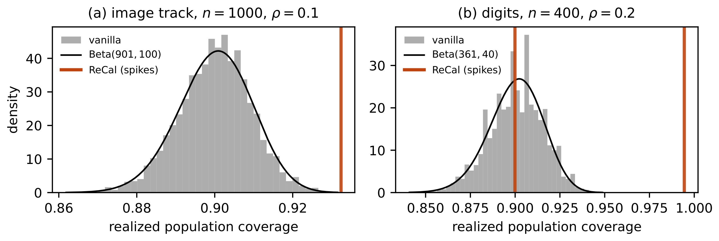
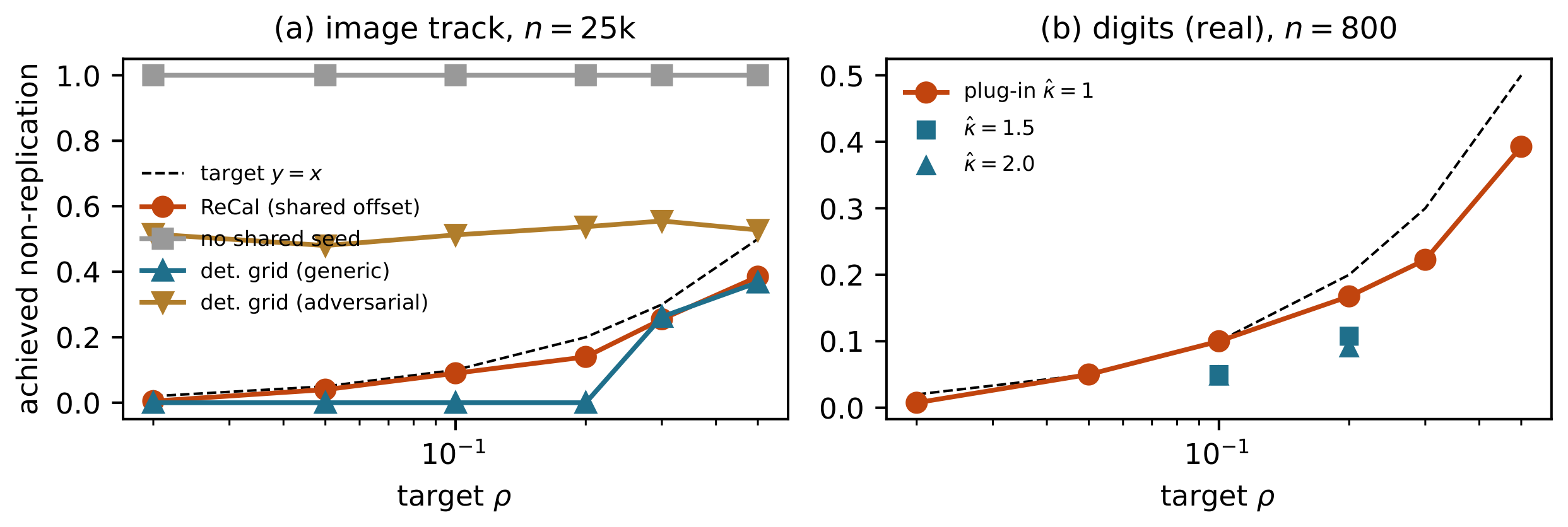
![**Figure 4:** **Measured sample-complexity frontier.** $\beta=\varepsilon/(2\hat{f})$ is fixed by $\varepsilon$ alone. (a) Mismatch vs. $n$: decay exponents $-.49, -.50, -.43, -.49$ across $\varepsilon$ (predicted $n^{-1/2}$); small- $\varepsilon$ curves saturate where the theory requires ($\beta\ll$ threshold spread). (b) $n^\ast$ vs. $1/(\varepsilon\rho)$ fits slope $2.09$ (CI $[1.99, 2.28]$; extrapolated points excluded), matching Corollary 7 and Theorem 13.](https://ittowtnkqtyixxjxrhou.supabase.co/storage/v1/object/public/public-images/ghzbhp5w/fig3_scaling.png)
\begin{tabular}{llcccc}
\toprule
  {} & Method & Coverage & Avg. size & Ident. & Agree \\
\midrule
\multirow{4}{*}{\shortstack[l]{digits\\($n{=}800$, \\$600 $pairs)}} & APS (derand.) &$.9001\pm.0109 $ & $ 1.08 $ & $.02 $ & $.98 $\\ & \textsc{ReCal}$ \rho{=}.2 $ & $.9365\pm.0233 $ & $ 1.12 $ & $.81 $ & $.98 $\\ & \textsc{ReCal}$ \rho{=}.1 $ & $.9626\pm.0341 $ & $ 3.65 $ & $.89 $ & $.88 $\\ & Det.-grid$ 2 $-list ($ \beta $ as $ \rho{=}.2 $) & $.9438\pm.0305 $ & $ 1.13 $ & $.63 $ & $.94 $ \\
\midrule
\multirow{5}{*}{\shortstack[l]{Llama-3.2-1B\\(real, WikiText, \\$n{=}5{,}000$, \\$100$pairs)}} & APS (derand.) &$.9000\pm.0044 $ & $ 83.7 $ & $.04 $ & $.55 $\\ & \textsc{ReCal}$ \rho{=}.1 $ & $.9297\pm.0183 $ & $ 132.8 $ & $.89 $ & $.93 $\\ & \textsc{ReCal}$ \rho{=}.05 $ & $.9573\pm.0299 $ & $ 10{,}586 $ & $.96 $ & $.92 $\\ & CRC top-$ p $ (standard) & $.9012\pm.0044 $ & $ 1084 $ & $.01 $ & $.19 $\\ & \textsc{ReCal}-CRC$ \rho{=}.1 $ & $.9356\pm.0140 $ & $ 12{,}717 $ & $.96 $ & $.96$ \\
\bottomrule
\end{tabular}
\begin{tabular}{llccccc}
\toprule
  {} & Method & Ident. & Agree & Jaccard & Churn (marg.) & Churn $\mid$ pair mism. (#) \\ \midrule \multirow{3}{*}{image} & derand. & $.02$ & $.66$ & $.92$ & $0.36$ & $0.37$   (59) \\ & bag- $10$ & $.00$ & $.63$ & $.91$ & $0.39$ & $0.39$   (60) \\ & \textsc{ReCal} $.1$ & $.97$ & $.97$ & $.94$ & $0.19$ & $5.82$   (2) \\ \midrule \multirow{3}{*}{digits} & derand. & $.05$ & $.98$ & $.92$ & $0.019$ & $0.02$   (57) \\ & bag- $10$ & $.00$ & $.98$ & $.92$ & $0.017$ & $0.02$   (60) \\ & \textsc{ReCal} $.1$ & $.93$ & $.93$ & $.92$ & $0.60$ & $9.01$   (4) \\ \midrule \multirow{3}{*}{\shortstack[l]{LLM\\(Llama-1B)}} & derand. & $.00$ & $.52$ & $.94$ & $5.0$ & $5.0$   (40) \\ & bag- $10$ & $.00$ & $.52$ & $.94$ & $4.8$ & $4.8$   (40) \\ & \textsc{ReCal} $.1$ & $.90$ & $.92$ & $.94$ & $15.1$ & $151$   (4) \\
\bottomrule
\end{tabular}
Environment and reproduction.
Every image-track, digits, frontier, attack, and synthetic-LM number in this paper regenerates deterministically in approximately three minutes on one CPU core; the four real-model tables regenerate from the cached logits in $6$ – $10$ CPU-minutes per model, and logit extraction itself used one GPU. The full suite was rerun end-to-end before finalizing this draft, and the paper reports that single run. All randomness derives from fixed master seeds (pool $20260808$, instance-jitter $777$, analyst resampling $424242$) with documented per-experiment offsets, and every pair's shared offset seed is derived deterministically. A common interface (an $(N, K)$ logit matrix with $(N)$ labels) substitutes real cached model outputs for the image and next-token generators with no other change. Next-token extraction computes logits on a WikiText-103 slice from locally cached checkpoints and has been verified end-to-end (measured test top-1: GPT-2 $.402$, Pythia-1.4B $.504$, Qwen2.5-1.5B $.519$, Llama-3.2-1B $.516$, consistent with published values for these models, and spanning vocabularies from $50$ k to $152$ k tokens); image extraction computes class logits from a ViT-Base checkpoint (google/vit-base-patch16-224) on an ImageNet-layout folder; memory scales as $N\times K\times2$ bytes in half precision ($\approx1$ GB for $10^{4}$ contexts at a $50$ k vocabulary).
Pools.
Image-classification testbed: $N{=}50{,}000$, $K{=}1{,}000$; labels uniform; per-example margin $\mu_i=\mathrm{softplus}(m+\xi_i)$, $\xi_i\sim\mathcal N(0, 1)$, with $m$ tuned by bisection (Gumbel approximation to the max of $K{-}1$ standard normals) to a top-1 of $0.78$; logits $z_i=\mu_ie_{y_i}+\mathcal N(0, I_K)$. Achieved top-1 $79.0%$, top-5 $89.9%$ (a real ResNet-152's top-5 is $\approx94%$; independent-coordinate logits thin the top-5 mass, a known limitation of this generator class). digits: scikit-learn digits, stratified $50/50$ split, multinomial logistic regression ($C{=}0.5$); pool = the $899$ held-out points; test accuracy $95.7%$. LLM-scale testbed: $N{=}10{,}000$, $K{=}8{,}192$; per-context Zipf (exponent $1.1$) logits under a random vocabulary permutation and per-context temperature $e^{0.35\mathcal N(0, 1)}$; labels drawn from the context distribution; the "model" sees temperature- $1.2$, noise-perturbed logits (deliberate miscalibration). Top-1 $8.9%$, mean entropy $7.0$ nats.
Scores and methods.
APS score $s_i=V_{i, o_i}-u_ip_{i, (o_i)}$ with $V$ the sorted-probability cumulative sums, $o_i$ the rank of the true label, and $u_i\in[0, 1)$ a fixed deterministic per-instance uniform (the hash surrogate of Remark 2; shared by all analysts, independent of calibration draws). "Fresh randomization" redraws $u$ per analyst and per test evaluation, as in the original APS. RAPS adds $\lambda\max(0, o-k_{\mathrm{reg}})$ with $(k_{\mathrm{reg}}, \lambda)=(5, 0.05)$. Thresholds use $k=\lceil(1-\alpha)(n+1)\rceil$; $\textsc{ReCal}$ rounds up on the shared offset grid; the seedless variant uses the fixed grid $\beta\mathbb Z$. Sizes and agreement metrics are computed from the monotone per-label score matrices on a fixed evaluation subsample ($10{,}000$ points on the image track, the full pool for digits; $4{,}000$ points for the synthetic, GPT-2, and Pythia pools and $2{,}000$ for Qwen and Llama): first $25$ pairs per configuration in Table 1–Table 3, $60$ pairs in Table 4. Coverage is computed on the full pool.
Grid rule.
$\beta=\hat\kappa\cdot\sqrt{2\alpha(1-\alpha)/n}, /(\hat{f}\rho)$ with $\hat{f}$ from a public pilot of $2{,}000$ pool draws (seed $1234$), window $\pm0.02$ around the pilot quantile; $\hat{f}=0.84$ (image), $1.31$ (digits), $0.75$ / $0.79$ (synthetic LLM testbed, APS/required-mass); per-model pilots for the real-LM runs are listed in the provenance paragraph above ($0.64$ – $1.15$ APS, $1.76$ – $4.38$ required-mass). $\hat\kappa=1$ unless stated; the paper's recommended default for deployment is $\hat\kappa=1.5$ (F2, Table 6).
Real LLM track: provenance and per-model details.
Logits were produced on locally cached checkpoints (single GPU, WikiText-103 test contexts of length $512$, half precision) and consumed through the common logits interface with no other change; suite runtime $6$ – $10$ minutes per model on one CPU core. Per model ($N$, $K$, top-1/top-5, entropy, APS pilot $\hat{f}$, mass-score pilot): GPT-2 ($10{,}000$, $50{,}257$, $.402/.624$, $3.59$ nats, $1.04$, $1.76$); Pythia-1.4B ($10{,}000$, $50{,}304$, $.504/.729$, $2.46$, $1.10$, $3.83$); Qwen2.5-1.5B ($10{,}000$, $151{,}936$, $.519/.754$, $2.18$, $0.64$, $4.35$); Llama-3.2-1B ($5{,}000$, $128{,}256$, $.516/.751$, $2.31$, $1.03$, $4.38$). Table 3 and Table 2 and the LLM rows of Table 4 and Table 6 come from these per-model runs, the LLM bars of Figure 1 from the Llama run, and every other number from the canonical synthetic-suite run. All nine per-model runs (the four families above and the five-point scale sweep below) produce mutually bit-identical image, digits, and frontier sections; the shared-seed design makes this checkable, and we verified it. Across machines, every discrete statistic reproduces exactly (the frontier slope to all printed digits, the attack counts, all fixed-pool thresholds) while floating-point aggregates agree to $\sim!10^{-5}$; the one genuine environment sensitivity is the digits track, which refits its logistic model at run time: a different scikit-learn build fits a marginally different model (test accuracy $.9555$ vs. $.9566$, pilot $\hat{f}$ $1.38$ vs. $1.31$), moving the $\rho{=}.1$ identity from $.887$ to $.930$; these alternate-build values come from a separate rerun. We disclose it, and it supplies a third independent stream for the Monte-Carlo paragraph below. For reference, the synthetic long-tail testbed at the matched operating point gives: APS derand. cov/size/ident/agree $.9005/2570/.01/.06$; $\textsc{ReCal}$ $\rho{=}.1$: $.9294/3108/.87/.84$ and $\rho{=}.05$: $.9539/4116/.98/.96$; CRC $.8997\to.9278$ with identity $.03\to.94$; spectrum churn $87\to80$ tokens; safety $.093/.053$ at $\hat\kappa{=}1/1.5$; the real models confirm this pattern qualitatively, except for the tail-geometry effect (F8) that only real vocabularies exhibit.
Model-scale sweep (Pythia $70$ M– $1.4$ B).
Five sizes of one family (one tokenizer, one $50{,}304$-token vocabulary, a $20\times$ parameter range) isolate the effect of model quality (Table 5, Figure 5). First, the protocol required no per-scale tuning across this sweep: the pilot density stays in $[0.96, 1.15]$ (the probability-integral-transform heuristic behind Assumption 5 holds at every scale), and the identical grid rule (same $\hat\kappa$, no per-model tuning) delivers identity $.85$ – $.94$ at $\rho{=}.1$ and $.94$ – $.96$ at $\rho{=}.05$, with $\hat\kappa{=}1.5$ at or below target everywhere except the $1.4$ B tie already noted. Second, within this sweep, scale alone does not produce replication: a $20\times$ larger model shrinks standard sets $559\to108$ tokens and lifts two-run agreement only from $.16$ to $.40$; larger models reduce churn, but exact agreement remains at most $.40$. The size cost varies non-monotonically within $46$ – $84%$, consistent with the tail-geometry effect of F8 at smaller magnitude.
\begin{tabular}{lccccccc}
\toprule
Model & Top-1 & Entropy & $\hat{f}$ & Std. size / agree & \textsc{ReCal} ident. & Cost & Non-rep. ($\hat\kappa{=}1.5$) \\ \midrule Pythia-70m & $.343$ & $3.89$ & $1.15$ & $559$ / $.16$ & $.87$ & $+46\%$ & $.070\pm.015$ \\ Pythia-160m & $.412$ & $3.53$ & $1.00$ & $342$ / $.28$ & $.85$ & $+47\%$ & $.060\pm.014$ \\ Pythia-410m & $.467$ & $2.75$ & $0.96$ & $162$ / $.32$ & $.89$ & $+65\%$ & $.070\pm.015$ \\ Pythia-1b & $.489$ & $2.54$ & $0.97$ & $127$ / $.38$ & $.94$ & $+84\%$ & $.033\pm.010$ \\ Pythia-1.4B & $.504$ & $2.46$ & $1.10$ & $108$ / $.40$ & $.93$ & $+58\%$ & $.103\pm.018$ \\
\bottomrule
\end{tabular}
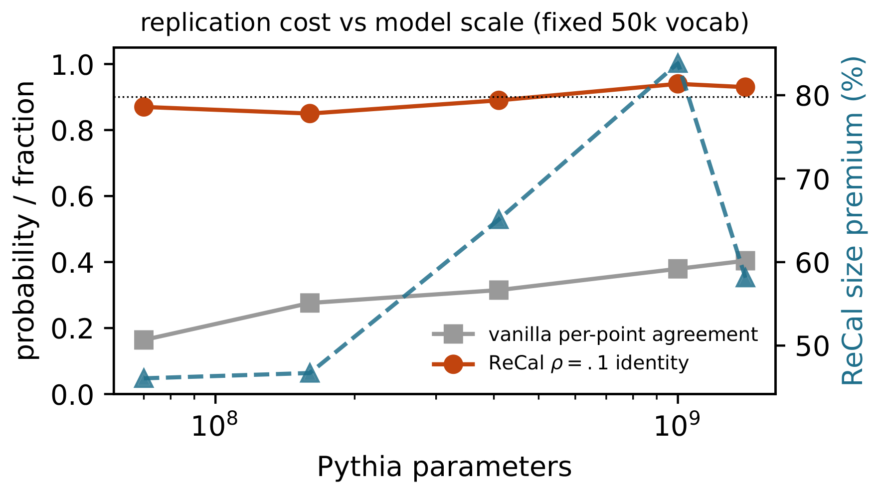
New experiments (specifications).
Spectrum (Table 4): $60$ pairs per track at $\rho{=}0.1$; per pair we compute exact set masks on the evaluation subsample and report identity, pointwise agreement, mean Jaccard (per test point $| \mathcal{C}\cap \mathcal{C}'|/\allowbreak\max{| \mathcal{C}\cup \mathcal{C}'|, 1}$, averaged over points and pairs), marginal churn $\mathbb{E}_X| \mathcal{C}\triangle \mathcal{C}'|$, and churn conditional on the pair mismatching (averaged over mismatching pairs only, with event counts; the marginal version, averaged over all pairs, would dilute rare events by construction). "bag- $10$ " recomputes each analyst's threshold as the mean of ten bootstrap-resample conformal quantiles of that analyst's own sample. Safety (Table 6): fresh pair streams, independent of the main tables ($400$ pairs per digits configuration, $300$ per LLM configuration). Cost curve (Figure 6): $40$ calibration draws per $\rho$, sizes on the first $15$.
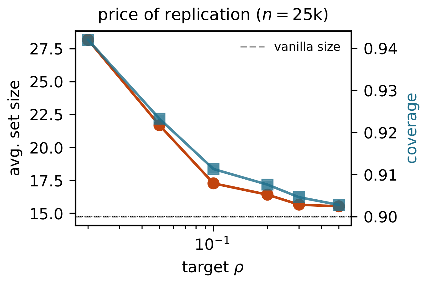
Sample-complexity frontier (Figure 4): $\varepsilon\in{.01, .02, .04, .08}$, $\beta=\varepsilon/(2\hat{f})$ fixed by $\varepsilon$ alone; $n$ on a $17$-point geometric grid $250\to64{,}000$; $600$ pairs per $(\varepsilon, n)$ cell measure the mismatch probability $p$ and the coverage inflation. Per $\varepsilon$, $\log p$ is regressed on $\log n$ over the unsaturated window $p\in[0.02, 0.45]$ (measured decay slopes $-0.49, -0.50, -0.43, -0.49$; the theoretical exponent is $-\tfrac12$); $n^{\ast}(\varepsilon, \rho)$ solves the fitted line at $p=\rho$. Six of the twelve $(\varepsilon, \rho)$ combinations resolve inside the measured grid and enter the frontier fit (slope $2.09$, bootstrap CI $[1.99, 2.28]$); two resolve just beyond it and are shown as open markers, excluded from the fit; four are censored beyond 1.28 x 10^5 and reported as such, exactly where the theory places them ($n^{\ast}\gtrsim7\times10^{5}$). The sweep holds $\alpha=0.1$ and $\kappa\approx1$ fixed: the $(\varepsilon\rho)^{-2}$ law is what is measured; the $\alpha(1-\alpha)$ and $\kappa^{2}$ factors of Corollary 7 and Theorem 13 are not separately probed. Selection attack (Figure 1 b): $n{=}5{,}000$, $M{=}20$ redraws, $300$ trials, pre-registered per-trial offset; the adversary deploys the draw with minimal population coverage (equivalently minimal sets, by monotonicity). At $\rho{=}0.1$: standard selected $.8920\pm.0024$ vs. honest $.9003$; $\textsc{ReCal}$ selected $.9170$ vs. honest $.9239$; $\ge2$ distinct $\textsc{ReCal}$ outputs in $30.7%$ of trials (the $(M{-}1)\rho{=}1.9$ union bound is vacuous here; the guarantee-preservation mechanism is what binds). At $\rho{=}0.01$: $\ge2$ distinct outputs in $1.3%$ of trials against the bound $19%$; selected $.9793$ vs. honest $.9797$. Risk control (Table 3): the required-mass score $M_i=V_{i, o_i}$ (cumulative sorted-probability mass through the true label, no jitter); $\hat\lambda$ is its conformal quantile (the CRC calibration of the monotone $0/1$ risk), and the deployed sets are ${y:\text{mass before }y<\hat\lambda}$ (calibrated top- $p$); $\textsc{ReCal}$ rounds $\hat\lambda$ on the shared grid in mass space; $100$ pairs. Corollary-level checks (image pool, $\rho{=}0.1$). Unequal calibration sizes (Corollary 8), $\beta$ set by the smaller analyst's rule: $(n_A, n_B)=(25\text{k}, 5\text{k})$ measures non-replication $.065\pm.012$ against the corollary's leading term $.102$, and $(25\text{k}, 1\text{k})$ measures $.052\pm.011$ against $.085$ ($400$ pairs each; both analysts'coverage $\ge.92$); the bound holds with $\approx1.6\times$ slack. Score mismatch (Corollary 25), analyst $B$ 's scores perturbed within sup norm $\eta_s$: the worst case (constant $+\eta_s$ shift) measures $.087/.123/.190$ at $\eta_s/\beta=.05/.1/.2$ against the additive bound $\text{base}+\eta_s/\beta=.143/.193/.293$ ($300$ pairs, base $.093\pm.017$), tracking the exact collision formula and converging to $\eta_s/\beta$ once $\eta_s$ exceeds the threshold spread; mean-zero noise of the same sup norm adds nothing ($.080$ – $.110$, statistically flat); the $\eta_s/\beta$ term is a sup-norm worst case, as stated. The population-mismatch term $\eta_P/f_{\min}$ and the membership bound of Corollary 25 remain analytic.
Real ImageNet run.
Cross-validated ResNet-50 predicted probabilities on the ILSVRC-2012 validation set ($N{=}50{,}000$, $K{=}1{,}000$; the float16-quantized probability matrix of [32]; recomputed top-1 $.727$, top-5 $.895$) enter the pipeline as $\log p$ logits; nothing else changes. At $n{=}25{,}000$, $100$ pairs: baseline identity $0.00$ (fresh and derandomized), agreement $.65/.87$, size $4.32$; $\textsc{ReCal}$ at $\rho{=}.1$: identity $.87$ ($\hat\kappa{=}1$; $.98$ at $\hat\kappa{=}1.5$), coverage $.910$, size $5.05$ ($+17%$); at $\rho{=}.01$: identity $.99$, size $13.2$; $\textsc{ReCal}$-RAPS $.94$ at $5.93$; seedless two-list mass $1.000$. Pilot $\hat{f}{=}2.03$.
Clinical site-split track.
The four UCI Heart Disease sites ([33]) (Cleveland Clinic $303$, Hungarian Institute of Cardiology $294$, V.A. Long Beach $200$, University Hospital Zurich $123$; CC BY 4.0; principal investigators A. Janosi, W. Steinbrunn, M. Pfisterer, R. Detrano). A logistic score on seven cross-site-complete features is trained on a public Cleveland split of $150$ patients ($.85$ training accuracy) and frozen, with deterministic instance jitter and a public pilot on the training scores ($\hat{f}{=}.67$); analysts calibrate on their own hospital with unequal sizes ($n_A{=}120$ Cleveland, $n_B{=}120$ – $200$ elsewhere; Corollary 8), $\hat\kappa{=}1.5$, $400$ trials. Baseline identity is $0.0$ for every pair. Cleveland–Budapest at $\rho{=}.3$: identity $.91$, per-site coverage $.982/.986$, sizes $1.84/1.89$ of $2$; at $\rho{=}.5$: identity $.84$, sizes $1.74/1.81$. Across all pairs (score Kolmogorov–Smirnov shift $.08$ – $.17$): identity $.78$ – $.96$, coverage $.97$ – $.99$. Identity is affordable at hospital scale only at coarse $\rho$ and near-vacuous sets: Corollary 14 in the field.
$\alpha$-dependence probe.
At fixed grid width $\beta^{\ast}$ (the protocol width at $\alpha{=}.1$, $\hat\kappa{=}1$) and $n{=}25{,}000$ on the image pool, mismatch was measured over $800$ pairs at each $\alpha\in{.05, .1, .2, .3, .4, .5}$ in two designs. On the raw APS score, whose pilot density at the working quantile varies $22\times$ over the sweep ($\hat{f}(q_\alpha)$ from $0.45$ to $9.7$), observed mismatch falls from $.069$ to $.0025$ and matches the plug-in prediction $B_n(\alpha)/(\hat{f}(q_\alpha)\beta^{\ast})$ with through-origin proportionality $0.97$ and $R^{2}=.99$: the bound's joint $(\alpha, f)$ structure holds at unit constant. On a rank-transformed copy of the pool ($f\equiv1$ exactly), which isolates the $\alpha(1-\alpha)$ factor, mismatch increases from $.028$ to $.073$ as predicted and lies below the theoretical bound $B_n(\alpha)/\beta^{\ast}$ at every level ($.037$ to $.083$; against $\sqrt{\alpha(1-\alpha)}$, $R^{2}=.54$ at $800$ pairs, binomial standard errors $\approx.008$).
Adaptive-limit check.
The limits of Proposition 12 are visible at the protocol's own scale. On the rank-transformed pool ($f\equiv1$, so the pilot ratio drops out), at $n{=}1.6\times10^{5}$, $\rho{=}.1$, $10^{4}$ pairs: mismatch $/\rho=.382\pm.019$ against the limit $\sqrt{2/\pi}/2\approx.399$; inflation $\times\rho/B_n$ equals $1.001$ – $1.005$ from $n{=}10^{4}$ on (limit $1$); and the $\sqrt{2/\pi}$ width of the last claim achieves mismatch $.100$ at the $\rho{=}.1$ target. On the raw APS score the pilot ratio enters as predicted: inflation $\times\rho/B_n$ rises $.56\to.93$ toward $f(q)/\hat{f}=1.04$, and mismatch $/\rho$ moves toward $.399, \hat{f}/f(q)=.38$ as $\beta_n\downarrow0$.
Finite-pool ties.
Because the "population" is a finite pool, redrawn indices repeat and standard thresholds can tie: the nonzero baseline identity rates ($\le.02$ image, $.02$ – $.05$ digits, $.00$ – $.04$ on the real LLMs, largest for Llama whose pool is $N{=}5{,}000$) are pool-atom artifacts that vanish for a continuous population (Proposition 3); they slightly help all methods equally.
\begin{tabular}{llcccc}
\toprule
  {} & Setting & $\hat\kappa$ & Non-rep. & Cov. inflation & Avg. size \\ \midrule \multirow{6}{*}{digits} & $\rho{=}0.1$ & $1.0$ & $0.075\pm0.013$ & $0.065$ & $3.79$ \\ & $\rho{=}0.1$ & $1.5$ & $0.050\pm0.011$ & $0.074$ & $2.89$ \\ & $\rho{=}0.1$ & $2.0$ & $0.048\pm0.011$ & $0.082$ & $6.47$ \\ & $\rho{=}0.2$ & $1.0$ & $0.160\pm0.018$ & $0.036$ & $1.11$ \\ & $\rho{=}0.2$ & $1.5$ & $0.107\pm0.015$ & $0.053$ & $1.15$ \\ & $\rho{=}0.2$ & $2.0$ & $0.090\pm0.014$ & $0.064$ & $4.67$ \\ \midrule \multirow{8}{*}{\shortstack[l]{LLM (real)\\all $\rho{=}0.1$}} & GPT-2 & $1.0$ & $0.103\pm0.018$ & $0.026$ & $526$ \\ & GPT-2 & $1.5$ & $0.050\pm0.013$ & $0.038$ & $589$ \\ & Pythia-1.4B & $1.0$ & $0.097\pm0.017$ & $0.027$ & $187$ \\ & Pythia-1.4B & $1.5$ & $0.103\pm0.018$ & $0.041$ & $253$ \\ & Qwen2.5-1.5B & $1.0$ & $0.060\pm0.014$ & $0.051$ & $15575$ \\ & Qwen2.5-1.5B & $1.5$ & $0.053\pm0.013$ & $0.063$ & $60880$ \\ & Llama-3.2-1B & $1.0$ & $0.073\pm0.015$ & $0.030$ & $139$ \\ & Llama-3.2-1B & $1.5$ & $0.043\pm0.012$ & $0.044$ & $147$ \\
\bottomrule
\end{tabular}
Monte Carlo precision.
Identity rates carry binomial standard errors: $.95$ over $100$ pairs is $\pm.022$; the digits $\rho{=}.1$ table entry ($.887$ over $600$ pairs, i.e. non-replication $.113\pm.013$) and the independent $400$-pair safety stream ($.075\pm.013$) are $2.1$ combined standard errors apart and bracket the $.10$ target; a full regeneration on a second machine, whose scikit-learn fit differs as noted above, gave $.070\pm.010$ on its own $600$-pair stream; the three independent streams straddle the target, reflecting the plug-in variability at $n{=}800$ and which makes $\hat\kappa{=}1.5$ the recommended default. A $0$-failure outcome over $100$ pairs (image track, $\rho{=}.01$) certifies only a $\le.03$ rate at $95%$ confidence by the rule of three; we state it as such.
References
Section Summary: This section compiles academic citations on statistical and machine learning methods for generating reliable predictions with uncertainty estimates. The works focus on conformal prediction approaches that provide distribution-free guarantees, alongside discussions of replicability, stability, and post-selection inference in models. Spanning foundational texts from the mid-2000s to recent conference papers and preprints through 2026, the references draw from statistics, computer science, and related fields.
[1] Vovk et al. (2005). Algorithmic learning in a random world. Springer.
[2] Lei et al. (2018). Distribution-free predictive inference for regression. Journal of the American Statistical Association. 113(523). pp. 1094–1111.
[3] Angelopoulos, Anastasios N and Bates, Stephen (2023). Conformal prediction: A gentle introduction. Foundations and Trends in Machine Learning. 16(4). pp. 494–591.
[4] Quach et al. (2024). Conformal language modeling. In International Conference on Learning Representations. pp. 11654–11681.
[5] Vovk, Vladimir (2012). Conditional validity of inductive conformal predictors. In Asian conference on machine learning. pp. 475–490.
[6] Berk et al. (2013). Valid post-selection inference. The Annals of Statistics. pp. 802–837.
[7] Taylor, Jonathan and Tibshirani, Robert J (2015). Statistical learning and selective inference. Proceedings of the National Academy of Sciences. 112(25). pp. 7629–7634.
[8] Fithian et al. (2014). Optimal inference after model selection. arXiv preprint arXiv:1410.2597.
[9] Prastalo, Gordan and Jablonka, Kevin Maik (2026). Reducing cross-sample prediction churn in scientific machine learning. arXiv preprint arXiv:2605.13826.
[10] Impagliazzo et al. (2022). Reproducibility in learning. In Proceedings of the 54th annual ACM SIGACT symposium on theory of computing. pp. 818–831.
[11] Bun et al. (2023). Stability is stable: Connections between replicability, privacy, and adaptive generalization. In Proceedings of the 55th Annual ACM Symposium on Theory of Computing. pp. 520–527.
[12] Dixon et al. (2023). List and certificate complexities in replicable learning. Advances in Neural Information Processing Systems. 36. pp. 30784–30806.
[13] Chase et al. (2023). Replicability and stability in learning. arXiv preprint arXiv:2304.03757.
[14] Hopkins et al. (2024). Replicability in high dimensional statistics. In 2024 IEEE 65th Annual Symposium on Foundations of Computer Science (FOCS). pp. 1–8.
[15] Ndiaye, Eugene (2022). Stable conformal prediction sets. In International Conference on Machine Learning. pp. 16462–16479.
[16] Romano et al. (2020). Classification with valid and adaptive coverage. Advances in neural information processing systems. 33. pp. 3581–3591.
[17] Angelopoulos et al. (2020). Uncertainty sets for image classifiers using conformal prediction. arXiv preprint arXiv:2009.14193.
[18] Chase et al. (2024). Local borsuk-ulam, stability, and replicability. In Proceedings of the 56th Annual ACM Symposium on Theory of Computing. pp. 1769–1780.
[19] Karbasi et al. (2023). Replicability in reinforcement learning. Advances in Neural Information Processing Systems. 36. pp. 74702–74735.
[20] Eaton et al. (2026). Replicable reinforcement learning with linear function approximation. In International Conference on Learning Representations. pp. 126582–126616.
[21] Liu, Sihan and Ye, Christopher (2024). Replicable uniformity testing. Advances in Neural Information Processing Systems. 37. pp. 32039–32075.
[22] Kalavasis et al. (2024). On the computational landscape of replicable learning. Advances in Neural Information Processing Systems. 37. pp. 105887–105927.
[23] Bian, Michael and Barber, Rina Foygel (2023). Training-conditional coverage for distribution-free predictive inference. Electronic Journal of Statistics. 17(2). pp. 2044–2066.
[24] Gupta et al. (2022). Nested conformal prediction and quantile out-of-bag ensemble methods. Pattern Recognition. 127. pp. 108496.
[25] Angelopoulos et al. (2024). Conformal risk control. In International conference on learning representations. pp. 55198–55218.
[26] Bashari et al. (2023). Derandomized novelty detection with FDR control via conformal e-values. Advances in Neural Information Processing Systems. 36. pp. 65585–65596.
[27] Balinsky, Alexander A and Balinsky, Alexander David (2025). When can we reuse a calibration set for multiple conformal predictions?. arXiv preprint arXiv:2506.19689.
[28] Scholten, Yan and Günnemann, Stephan (2025). Provably reliable conformal prediction sets in the presence of data poisoning. In International Conference on Learning Representations. pp. 55873–55897.
[29] Angelopoulos et al. (2022). Private prediction sets. Harvard Data Science Review. 4(2).
[30] Milani Fard et al. (2016). Launch and iterate: Reducing prediction churn. Advances in Neural Information Processing Systems. 29.
[31] Marx et al. (2020). Predictive multiplicity in classification. In International conference on machine learning. pp. 6765–6774.
[32] Northcutt et al. (2021). Pervasive label errors in test sets destabilize machine learning benchmarks. arXiv preprint arXiv:2103.14749.
[33] Detrano et al. (1989). International application of a new probability algorithm for the diagnosis of coronary artery disease. The American journal of cardiology. 64(5). pp. 304–310.
[34] Van der Vaart, Aad W (2000). Asymptotic statistics. Cambridge university press.