Learning Multiple Layers of Features from Tiny Images

Alex Krizhevsky
April 8, 2009

Abstract

Groups at MIT and NYU have collected a dataset of millions of tiny colour images from the web. It is, in principle, an excellent dataset for unsupervised training of deep generative models, but previous researchers who have tried this have found it difficult to learn a good set of filters from the images. We show how to train a multi-layer generative model that learns to extract meaningful features which resemble those found in the human visual cortex. Using a novel parallelization algorithm to distribute the work among multiple machines connected on a network, we show how training such a model can be done in reasonable time.

A second problematic aspect of the tiny images dataset is that there are no reliable class labels which makes it hard to use for object recognition experiments. We created two sets of reliable labels. The CIFAR-10 set has 6000 examples of each of 10 classes and the CIFAR-100 set has 600 examples of each of 100 non-overlapping classes. Using these labels, we show that object recognition is significantly improved by pre-training a layer of features on a large set of unlabeled tiny images.

Executive Summary: This report explores challenges in computer vision, particularly how machines can automatically learn meaningful patterns from vast collections of small, unlabeled images scraped from the web. In 2009, as digital images proliferated online, researchers faced a key problem: traditional methods struggled to extract useful features like edges or shapes from noisy, low-resolution data without extensive human labeling. This limited progress in applications like object recognition, which requires distinguishing everyday items such as animals or vehicles amid cluttered scenes. Addressing this now matters because it paves the way for more efficient AI systems that mimic human visual processing, reducing reliance on costly labeled datasets and enabling broader use in search engines, robotics, and surveillance.

The document aims to demonstrate how to train multi-layer generative models—energy-based systems called Restricted Boltzmann Machines (RBMs) stacked into Deep Belief Networks (DBNs)—to discover interpretable features from millions of tiny, unlabeled color images. It also evaluates whether these features boost performance in supervised object recognition tasks.

The authors analyzed a dataset of 80 million 32x32 pixel color images collected via web searches for English nouns, focusing experiments on a subset of about 2 million images from 2008. To preprocess, they applied a whitening transformation to reduce pixel correlations and noise, removing the 1,000 least variable directions while preserving image appearance. Initial training used small 8x8 image patches to simplify learning, then scaled to full images. Models learned features greedily, layer by layer, via an approximation called Contrastive Divergence over hundreds of training epochs. For classification tests, they created CIFAR-10—a reliable labeled set of 60,000 images across 10 classes like airplanes and cats, verified by human labelers—and compared methods like logistic regression and neural networks. A novel parallel algorithm distributed training across multiple machines and cores, enabling feasible computation times for large models with 10,000 hidden units.

Key results show the models successfully learned biologically plausible features. First, RBMs trained on patches produced localized edge detectors and low-frequency color filters, outperforming prior attempts that yielded only noisy or uniform patterns. Second, full-image training on unwhitened data evolved from initial "point-like" copies to broader edge and texture detectors, with learned pixel variances enabling higher-frequency details. Third, pre-training classifiers on these features dramatically improved accuracy: logistic regression on raw pixels hit about 40% on CIFAR-10 test sets, but on RBM features it reached 58-60%, a 50% relative gain; neural networks initialized from RBMs pushed this to 62% while converging in half the epochs of random starts. Fourth, a second RBM layer on first-layer features detected oriented edges and oppositions (e.g., favoring one edge direction over its mirror). Finally, the parallel training scaled nearly linearly: with 8 machines, it doubled speed for binary data and nearly so for continuous pixels, with communication costs under 50 MB per machine per batch.

These findings imply that unsupervised pre-training captures robust, human-like visual hierarchies, enhancing recognition by focusing on essential structures rather than pixel noise. This cuts risks of overfitting on small labeled sets, speeds development timelines, and improves performance in real-world scenarios with limited supervision—potentially lowering costs for vision systems by 20-50% through reduced labeling needs. Unlike earlier failures, success here stemmed from preprocessing and patch training, highlighting how data preparation unlocks deeper learning; it challenges assumptions that raw web data is unusable without heavy cleaning.

Leaders should adopt RBM pre-training for image classification pipelines, integrating it with neural networks for quick gains on similar low-res tasks. Trade-offs include higher upfront compute for pre-training versus faster end-to-end supervised baselines. Next, pilot deeper DBNs on expanded datasets like CIFAR-100 (100 classes, 60,000 images) or larger images to test scalability, and explore real-time applications in mobile vision.

Confidence in these results is high for small, noisy images, backed by consistent replication across experiments, but caution applies: the tiny size limits fine details like textures, web data introduces label noise, and Contrastive Divergence approximations may undervalue rare patterns. Further validation on diverse, high-res datasets would strengthen generalizability.

Chapter 1: Preliminaries

Section Summary: This chapter introduces the basics of training multi-layer generative models, like Restricted Boltzmann Machines and Deep Belief Networks, on a massive dataset of tiny 32x32 color images collected from web searches of everyday objects, totaling 80 million images with a subset of 2 million used for experiments. It highlights key properties of natural images, such as strong correlations between nearby pixels, color channel similarities, and symmetries from how photos are taken, which appear in the dataset's covariance matrix. To help models focus on complex patterns rather than simple pixel similarities, the chapter describes a ZCA whitening transformation that decorrelates pixels beforehand, visualized as local filters.

1.1 Introduction

In this work we describe how to train a multi-layer generative model of natural images. We use a dataset of millions of tiny colour images, described in the next section. This has been attempted by several groups but without success[3, 7]. The models on which we focus are RBMs (Restricted Boltzmann Machines) and DBNs (Deep Belief Networks). These models learn interesting-looking filters, which we show are more useful to a classifier than the raw pixels. We train the classifier on a labeled subset that we have collected and call the CIFAR-10 dataset.

1.2 Natural images

1.2.1 The dataset

The tiny images dataset on which we based all of our experiments was collected by colleagues at MIT and NYU over the span of six months; it is described in detail in [14]. They assembled it by searching the web for images of every non-abstract English noun in the lexical database WordNet[15, 8]. They used several search engines, including Google, Flickr, and Altavista and kept roughly the first 3000 results for each search term. After collecting all the images for a particular search term, they removed perfect duplicates and images in which an excessively large portion of the pixels were white, as they tended to be synthetic figures rather than natural images. The search term used to find an image provides it with a rough label, although it is extremely unreliable due to the nature of online image search technology.

In total, the dataset contains 80 million colour images downscaled to $32 \times 32$ and spread out across 79000 search terms. Most of our experiments with unsupervised learning were performed on a subset of about 2 million images.

1.2.2 Properties

Real images have various properties that other datasets do not. Many of these properties can be made apparent by examining the covariance matrix of the tiny images dataset. Figures 1.1 and 1.2 show this covariance matrix.

The main diagonal and its neighbours demonstrate the most apparent feature of real images: pixels are strongly correlated to nearby pixels and weakly correlated to faraway pixels. Various other properties can be observed as well, for example:

• The green value of one pixel is highly correlated to the green value of a neighbouring pixel, but slightly less correlated to the blue and red values of the neighbouring pixel.

• The images tend to be symmetric about the vertical and horizontal. For example, the colour of the top-left pixel is correlated to the colour of the top-right pixel and the bottom-left pixel. This kind of symmetry can be observed in all pixels in the faint anti-diagonals of the covariance matrix. It is probably caused by the way people take photographs – making the ground plane horizontal and centering on the main object.

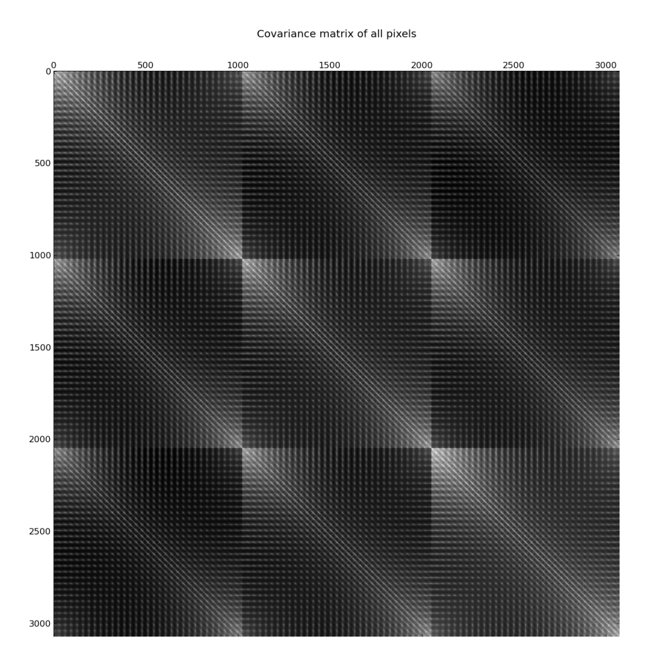
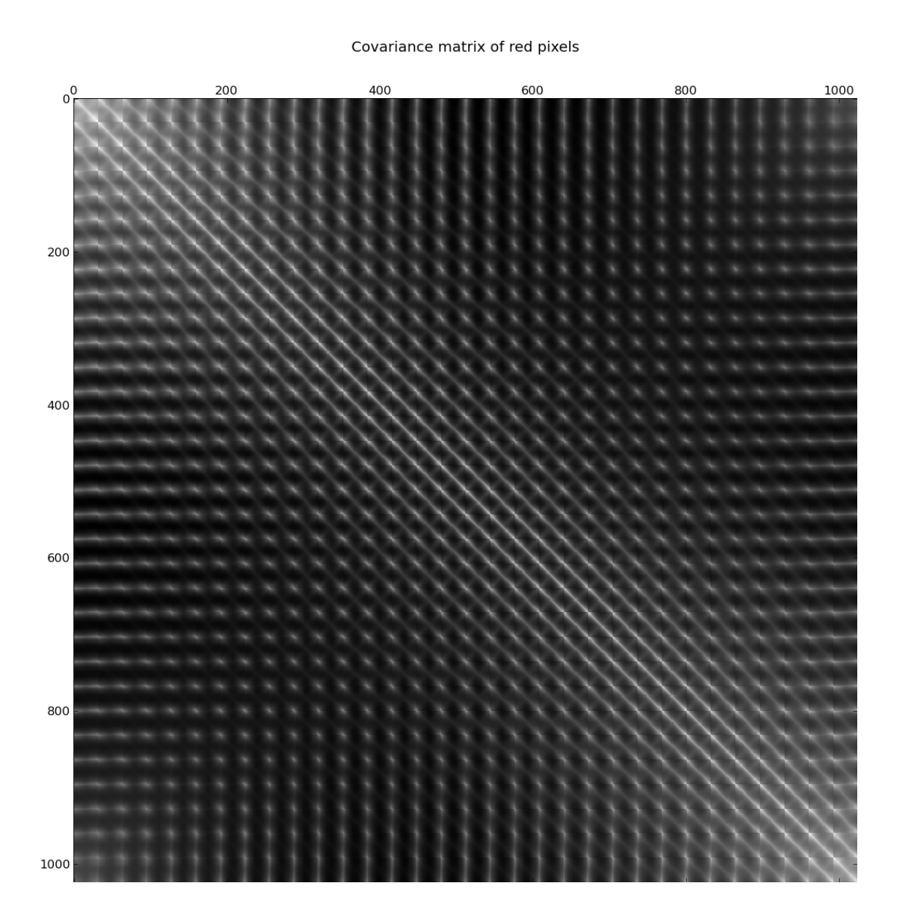
• As an extension of the above point, pixels are much more correlated with faraway pixels in the same row or column than with faraway pixels in a different row or column.

1.3 The ZCA whitening transformation

1.3.1 Motivation

As mentioned above, the tiny images exhibit strong correlations between nearby pixels. In particular, two-way correlations are quite strong. When learning a statistical model of images, it might be nice to force the model to focus on higher-order correlations rather than get distracted by modelling two-way correlations. The hypothesis is that this might make the model more likely to discover interesting regularities in the images rather than merely learn that nearby pixels are similar.[^1]

[^1]: Here when we say pixel, we are really referring to a particular colour channel of a pixel. The transformation we will describe decorrelates the value of a particular colour channel in a particular pixel from the value of another colour channel in another (or possibly the same) pixel. It does not decorrelate the values of all three colour channels in one pixel from the values of all three in another pixel.

One way to force the model to ignore second-order structure is to remove it. Luckily this can be done with a data preprocessing step that just consists of multiplying the data matrix by a whitening matrix. After the transformation, it will be impossible to predict the value of one pixel given the value of only one other pixel, so any statistical model would be wise not to try. The transformation is described in Appendix A.

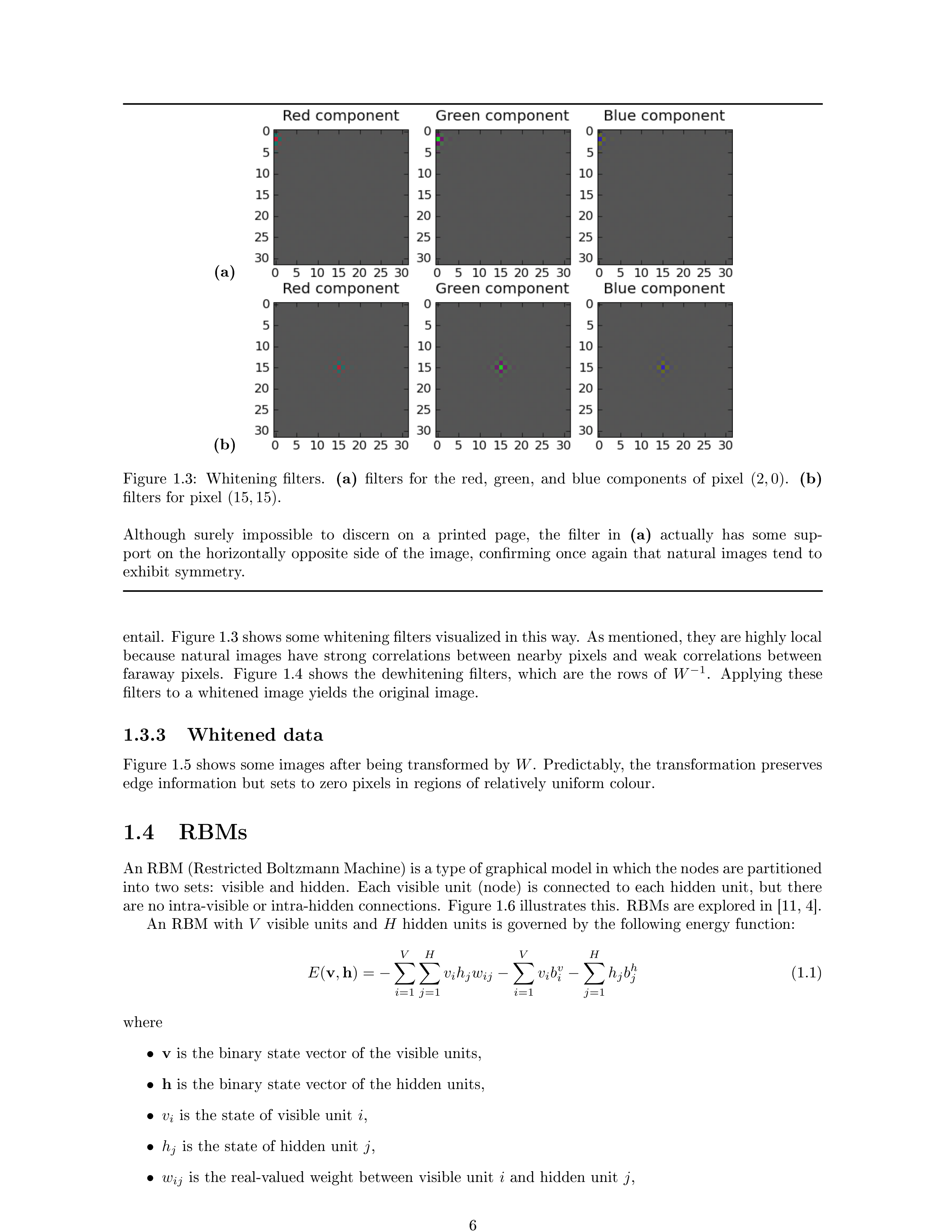
1.3.2 Whitening filters

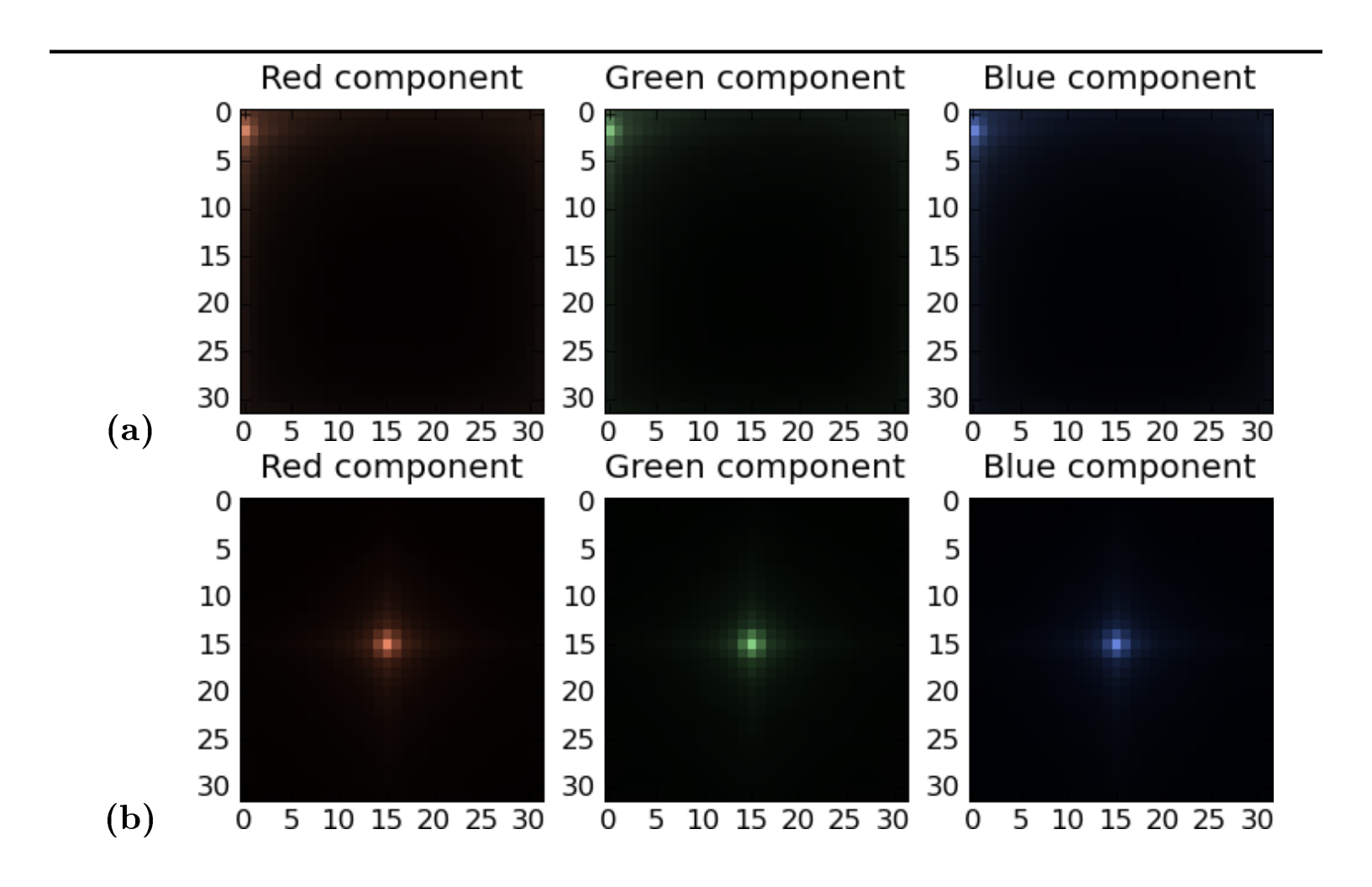
Using the notation of Appendix A, where $W$ is the whitening matrix, each row $W_i$ of $W$ can be thought of as a filter that is applied to the data points by taking the dot product of the filter $W_i$ and the data point $X_j$. If, as in our case, the data points are images, then each filter has exactly as many "pixels" as do the images, and so it is natural to try to visualize these filters to see the kinds of transformations they entail. Figure 1.3 shows some whitening filters visualized in this way. As mentioned, they are highly local because natural images have strong correlations between nearby pixels and weak correlations between faraway pixels. Figure 1.4 shows the dewhitening filters, which are the rows of $W^{-1}$. Applying these filters to a whitened image yields the original image.

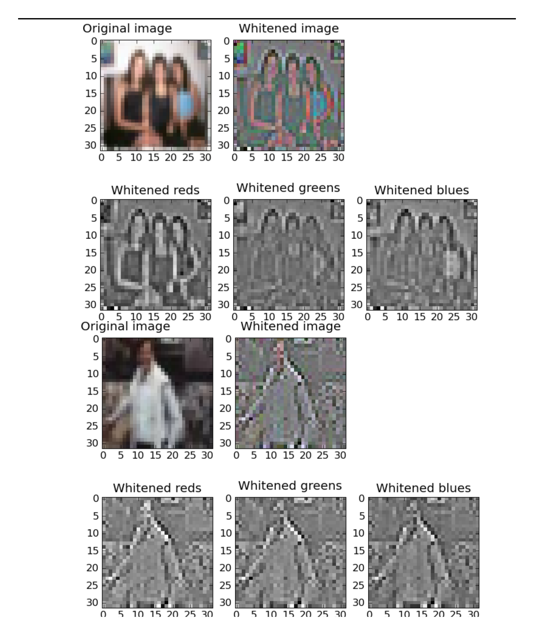
1.3.3 Whitened data

Figure 1.5 shows some images after being transformed by $W$. Predictably, the transformation preserves edge information but sets to zero pixels in regions of relatively uniform colour.

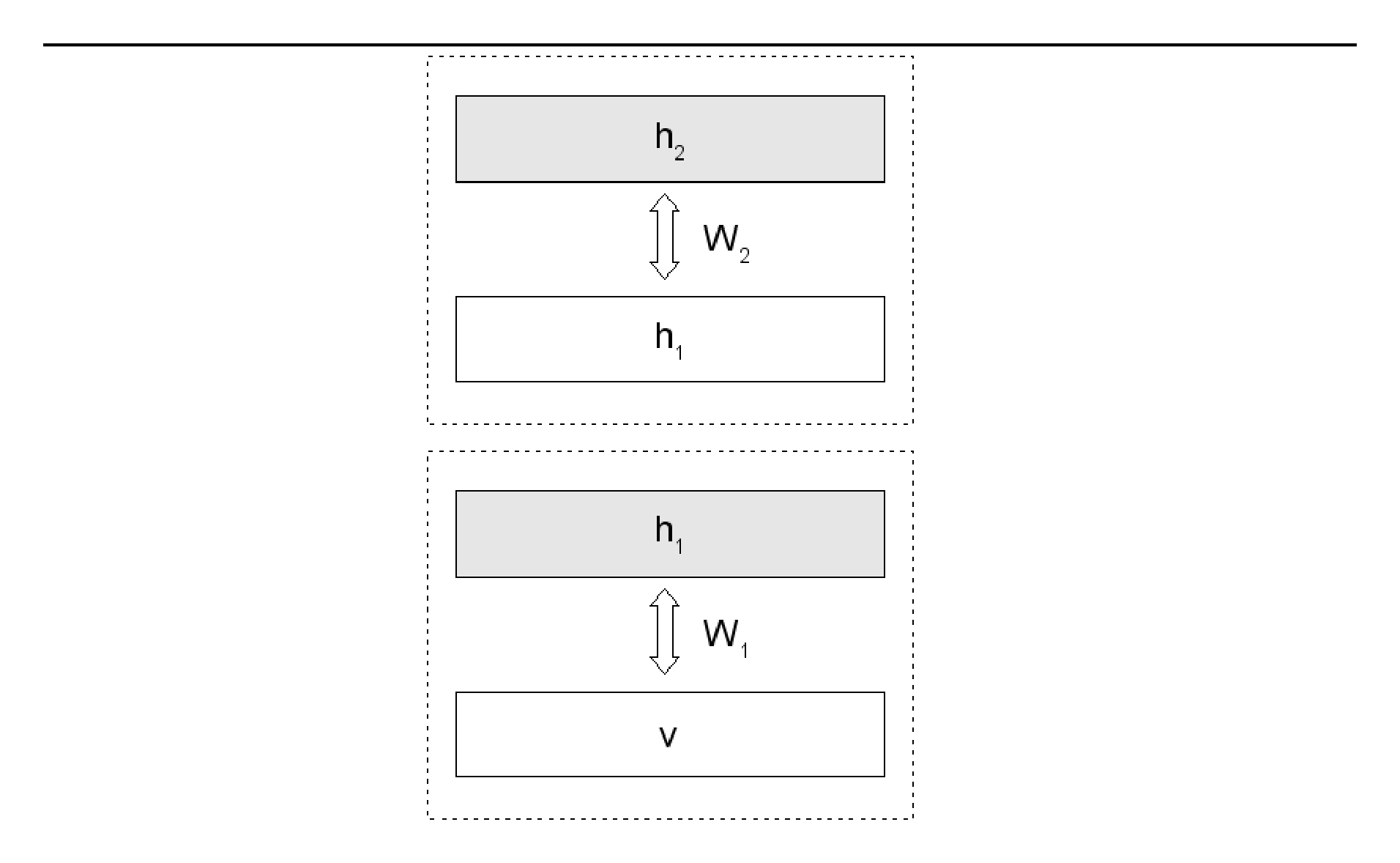
1.4 RBMs

An RBM (Restricted Boltzmann Machine) is a type of graphical model in which the nodes are partitioned into two sets: visible and hidden. Each visible unit (node) is connected to each hidden unit, but there are no intra-visible or intra-hidden connections. Figure 1.6 illustrates this. RBMs are explored in [11, 4].

An RBM with $V$ visible units and $H$ hidden units is governed by the following energy function:

$ E(\mathbf{v}, \mathbf{h}) = -\sum_{i=1}^{V}\sum_{j=1}^{H} v_i h_j w_{ij} - \sum_{i=1}^{V} v_i b_i^v - \sum_{j=1}^{H} h_j b_j^h \tag{1.1} $

where

• $\mathbf{v}$ is the binary state vector of the visible units,
• $\mathbf{h}$ is the binary state vector of the hidden units,
• $v_i$ is the state of visible unit $i$,
• $h_j$ is the state of hidden unit $j$,
• $w_{ij}$ is the real-valued weight between visible unit $i$ and hidden unit $j$,
• $b_i^v$ is the real-valued bias into visible unit $i$,
• $b_j^h$ is the real-valued bias into hidden unit $j$.

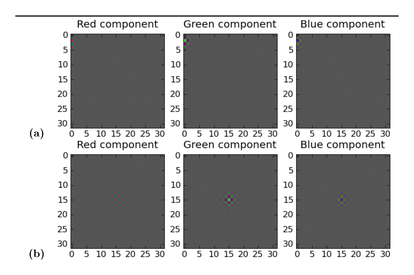
Although surely impossible to discern on a printed page, the filter in (a) actually has some support on the horizontally opposite side of the image, confirming once again that natural images tend to exhibit symmetry.

A probability is associated with configuration $(\mathbf{v}, \mathbf{h})$ as follows:

$ p(\mathbf{v}, \mathbf{h}) = \frac{e^{-E(\mathbf{v}, \mathbf{h})}}{\sum_{\mathbf{u}} \sum_{\mathbf{g}} e^{-E(\mathbf{u}, \mathbf{g})}}. \tag{1.2} $

Intuitively, configurations with low energy are assigned high probability and configurations with high energy are assigned low probability. The sum in the denominator is over all possible visible and hidden configurations, and is thus extremely hard to compute when the number of units is large.

The probability of a particular visible state configuration $\mathbf{v}$ is derived as follows:

$ \begin{aligned} p(\mathbf{v}) &= \sum_{\mathbf{g}} p(\mathbf{v}, \mathbf{g}) \ &= \frac{\sum_{\mathbf{g}} e^{-E(\mathbf{v}, \mathbf{g})}}{\sum_{\mathbf{u}} \sum_{\mathbf{g}} e^{-E(\mathbf{u}, \mathbf{g})}}. \end{aligned} \tag{1.3} $

At a very high-level, the RBM training procedure consists of fixing the states of the visible units $\mathbf{v}$ at some desired configuration and then finding settings of the parameters (the weights and biases) such that $p(\mathbf{v})$ is large. The hope is that the model will use the hidden units to generalize and to extract meaningful features from the data, and hence $p(\mathbf{u})$ will also be large for $\mathbf{u}$ drawn from the same distribution as $\mathbf{v}$.

We now derive a few other distributions that are entailed by equation (1.2). The formula for $p(\mathbf{h})$ is entirely analogous to that of $p(\mathbf{v})$:

$ p(\mathbf{h}) = \frac{\sum_{\mathbf{u}} e^{-E(\mathbf{u}, \mathbf{h})}}{\sum_{\mathbf{u}} \sum_{\mathbf{g}} e^{-E(\mathbf{u}, \mathbf{g})}}. $

We can also derive some simple conditional expressions:

$ \begin{aligned} p(\mathbf{v}|\mathbf{h}) &= \frac{p(\mathbf{v}, \mathbf{h})}{p(\mathbf{h})} \ &= \frac{e^{-E(\mathbf{v}, \mathbf{h})}}{\sum_{\mathbf{u}} e^{-E(\mathbf{u}, \mathbf{h})}} \ p(\mathbf{h}|\mathbf{v}) &= \frac{p(\mathbf{v}, \mathbf{h})}{p(\mathbf{v})} \ &= \frac{e^{-E(\mathbf{v}, \mathbf{h})}}{\sum_{\mathbf{g}} e^{-E(\mathbf{v}, \mathbf{g})}}. \end{aligned} $

We can also derive a closed-form expression for $p(v_k = 1|\mathbf{h})$, the probability of a particular visible unit being on given a hidden configuration. To do this, we introduce the notation

$ p(v_k = 1, \mathbf{v}_{i \neq k}, \mathbf{h}) $

to denote the probability of the configuration in which visible unit $k$ has state 1, the rest of the visible units have state $\mathbf{v}_{i \neq k}$, and the hidden units have state $\mathbf{h}$. Given this, we have

$ \begin{aligned} p(v_k = 1|\mathbf{h}) &= \frac{p(v_k = 1, \mathbf{h})}{p(\mathbf{h})} \ &= \frac{\sum_{\mathbf{v}{i \neq k}} p(v_k = 1, \mathbf{v}{i \neq k}, \mathbf{h})}{p(\mathbf{h})} \ &= \frac{\sum_{\mathbf{v}{i \neq k}} \frac{e^{-E(v_k=1, \mathbf{v}{i \neq k}, \mathbf{h})}}{\sum_{\mathbf{u}} \sum_{\mathbf{g}} e^{-E(\mathbf{u}, \mathbf{g})}}}{\frac{\sum_{\mathbf{u}} e^{-E(\mathbf{u}, \mathbf{h})}}{\sum_{\mathbf{u}} \sum_{\mathbf{g}} e^{-E(\mathbf{u}, \mathbf{g})}}} \ &= \frac{\sum_{\mathbf{v}{i \neq k}} e^{-E(v_k=1, \mathbf{v}{i \neq k}, \mathbf{h})}}{\sum_{\mathbf{u}} e^{-E(\mathbf{u}, \mathbf{h})}} \ &= \frac{\sum_{\mathbf{v}{i \neq k}} e^{(\sum{j=1}^{H} h_j w_{kj} + b_k^v) + (\sum_{i \neq k}^{V} \sum_{j=1}^{H} v_i h_j w_{ij} + \sum_{i \neq k}^{V} v_i b_i^v + \sum_{j=1}^{H} h_j b_j^h)}}{\sum_{\mathbf{u}} e^{-E(\mathbf{u}, \mathbf{h})}} \ &= \frac{[e^{(\sum_{j=1}^{H} h_j w_{kj} + b_k^v)}] \sum_{\mathbf{v}{i \neq k}} e^{(\sum{i \neq k}^{V} \sum_{j=1}^{H} v_i h_j w_{ij} + \sum_{i \neq k}^{V} v_i b_i^v + \sum_{j=1}^{H} h_j b_j^h)}}{\sum_{\mathbf{u}} e^{-E(\mathbf{u}, \mathbf{h})}} \ &= \frac{[e^{(\sum_{j=1}^{H} h_j w_{kj} + b_k^v)}] \sum_{\mathbf{v}{i \neq k}} e^{-E(v_k=0, \mathbf{v}{i \neq k}, \mathbf{h})}}{\sum_{\mathbf{u}} e^{-E(\mathbf{u}, \mathbf{h})}} \ &= \frac{[e^{(\sum_{j=1}^{H} h_j w_{kj} + b_k^v)}] \sum_{\mathbf{v}{i \neq k}} e^{-E(v_k=0, \mathbf{v}{i \neq k}, \mathbf{h})}}{\sum_{\mathbf{u}{i \neq k}} e^{-E(u_k=1, \mathbf{u}{i \neq k}, \mathbf{h})} + \sum_{\mathbf{u}{i \neq k}} e^{-E(u_k=0, \mathbf{u}{i \neq k}, \mathbf{h})}} \ &= \frac{[e^{(\sum_{j=1}^{H} h_j w_{kj} + b_k^v)}] \sum_{\mathbf{v}{i \neq k}} e^{-E(v_k=0, \mathbf{v}{i \neq k}, \mathbf{h})}}{[e^{(\sum_{j=1}^{H} h_j w_{kj} + b_k^v)}] \sum_{\mathbf{u}{i \neq k}} e^{-E(u_k=0, \mathbf{u}{i \neq k}, \mathbf{h})} + \sum_{\mathbf{u}{i \neq k}} e^{-E(u_k=0, \mathbf{u}{i \neq k}, \mathbf{h})}} \ &= \frac{1}{1 + e^{-(\sum_{j=1}^{H} h_j w_{kj} + b_k^v)}}. \end{aligned} $

Likewise,

$ p(h_k = 1|\mathbf{v}) = \frac{1}{1 + e^{-(\sum_{i=1}^{V} v_i w_{ik} + b_k^h)}}. \tag{1.4} $

So as can be expected from Figure 1.6, we find that the probability of a visible unit turning on is independent of the states of the other visible units, given the states of the hidden units. Likewise, the hidden states are independent of each other given the visible states. This property of RBMs makes sampling extremely efficient, as one can sample all the hidden units simultaneously and then all the visible units simultaneously.

1.4.1 Training RBMs

Given a set of $C$ training cases ${\mathbf{v}^c|c \in {1, \dots, C}}$, the goal is to maximize the average log probability of the set under the model's distribution:

$ \sum_{c=1}^{C} \log p(\mathbf{v}^c) = \sum_{c=1}^{C} \log \frac{\sum_{\mathbf{g}} e^{-E(\mathbf{v}^c, \mathbf{g})}}{\sum_{\mathbf{u}} \sum_{\mathbf{g}} e^{-E(\mathbf{u}, \mathbf{g})}}. $

We attempt to do this with gradient descent. Differentiating with respect to a weight $w_{ij}$, we have

$ \begin{aligned} \frac{\partial}{\partial w_{ij}} \sum_{c=1}^{C} \log p(\mathbf{v}^c) &= \frac{\partial}{\partial w_{ij}} \sum_{c=1}^{C} \log \frac{\sum_{\mathbf{g}} e^{-E(\mathbf{v}^c, \mathbf{g})}}{\sum_{\mathbf{u}} \sum_{\mathbf{g}} e^{-E(\mathbf{u}, \mathbf{g})}} \ &= \frac{\partial}{\partial w_{ij}} \left( \sum_{c=1}^{C} \log \sum_{\mathbf{g}} e^{-E(\mathbf{v}^c, \mathbf{g})} - \log \sum_{\mathbf{u}} \sum_{\mathbf{g}} e^{-E(\mathbf{u}, \mathbf{g})} \right). \end{aligned} \tag{1.5} $

First consider the first term:

$ \begin{aligned} \frac{\partial}{\partial w_{ij}} \sum_{c=1}^{C} \log \sum_{\mathbf{g}} e^{-E(\mathbf{v}^c, \mathbf{g})} &= \sum_{c=1}^{C} \frac{\frac{\partial}{\partial w_{ij}} \sum_{\mathbf{g}} e^{-E(\mathbf{v}^c, \mathbf{g})}}{\sum_{\mathbf{g}} e^{-E(\mathbf{v}^c, \mathbf{g})}} \ &= -\sum_{c=1}^{C} \frac{\sum_{\mathbf{g}} e^{-E(\mathbf{v}^c, \mathbf{g})} \frac{\partial E(\mathbf{v}^c, \mathbf{g})}{\partial w_{ij}}}{\sum_{\mathbf{g}} e^{-E(\mathbf{v}^c, \mathbf{g})}} \ &= -\sum_{c=1}^{C} \frac{\sum_{\mathbf{g}} e^{-E(\mathbf{v}^c, \mathbf{g})} v_i^c g_j}{\sum_{\mathbf{g}} e^{-E(\mathbf{v}^c, \mathbf{g})}}. \end{aligned} $

Notice that the term $\frac{\sum_{\mathbf{g}} e^{-E(\mathbf{v}^c, \mathbf{g})} v_i^c g_j}{\sum_{\mathbf{g}} e^{-E(\mathbf{v}^c, \mathbf{g})}}$ is just the expected value of $v_i^c g_j$ given that $\mathbf{v}$ is clamped to the data vector $\mathbf{v}^c$. This is easy to compute since we know $v_i^c$ and we can compute the expected value of $g_j$ using equation (1.4).

Turning our attention to the second term in equation (1.5):

$ \begin{aligned} \frac{\partial}{\partial w_{ij}} \sum_{c=1}^{C} \log \sum_{\mathbf{u}} \sum_{\mathbf{g}} e^{-E(\mathbf{u}, \mathbf{g})} &= \sum_{c=1}^{C} \frac{\frac{\partial}{\partial w_{ij}} \sum_{\mathbf{u}} \sum_{\mathbf{g}} e^{-E(\mathbf{u}, \mathbf{g})}}{\sum_{\mathbf{u}} \sum_{\mathbf{g}} e^{-E(\mathbf{u}, \mathbf{g})}} \ &= -\sum_{c=1}^{C} \frac{\sum_{\mathbf{u}} \sum_{\mathbf{g}} e^{-E(\mathbf{u}, \mathbf{g})} \frac{\partial E(\mathbf{u}, \mathbf{g})}{\partial w_{ij}}}{\sum_{\mathbf{u}} \sum_{\mathbf{g}} e^{-E(\mathbf{u}, \mathbf{g})}} \ &= -\sum_{c=1}^{C} \frac{\sum_{\mathbf{u}} \sum_{\mathbf{g}} e^{-E(\mathbf{u}, \mathbf{g})} u_i g_j}{\sum_{\mathbf{u}} \sum_{\mathbf{g}} e^{-E(\mathbf{u}, \mathbf{g})}}. \end{aligned} \tag{1.6} $

Here, the term $\frac{\sum_{\mathbf{u}} \sum_{\mathbf{g}} e^{-E(\mathbf{u}, \mathbf{g})} u_i g_j}{\sum_{\mathbf{u}} \sum_{\mathbf{g}} e^{-E(\mathbf{u}, \mathbf{g})}}$ is the expected value of $u_i g_j$ under the model's distribution. We can compute $u_i g_j$ by clamping the visible units at the data vector $\mathbf{v}^c$, then sampling the hidden units, then sampling the visible units, and repeating this procedure infinitely many times. After infinitely many iterations, the model will have forgotten its starting point and we will be sampling from its equilibrium distribution. However, it has been shown in [5] that this expectation can be approximated in finite time by a procedure known as Contrastive Divergence (CD). The CD learning procedure approximates (1.6) by running the sampling chain for only a few steps. It is illustrated in Figure 1.7. We name CD-$N$ the algorithm that samples the hidden units $N + 1$ times.

In practice, we use CD-1 almost exclusively because it produces adequate results. CD-1 learning amounts to lowering the energy that the model assigns to training vectors and raising the energy of the model's "reconstructions" of those training vectors. It has the potential pitfall that places in the energy surface that are nowhere near data do not get explicitly modified by the algorithm, although they are affected by the changes in parameters that CD-1 induces.

Renaming $g$s to $h$s, the update rule for weight $w_{ij}$ is

$ \Delta w_{ij} = \epsilon_w (E_{data}[v_i h_j] - E_{model}[v_i h_j]) $

where $\epsilon_w$ is the weight learning rate hyperparameter, $E_{data}$ is the expectation under the model's distribution when the the visible units are clamped to the data, and $E_{model}$ is the expectation under the model's distribution when the visible units are unclamped. As discussed above, $E_{model}$ is approximated using CD.

The update rules for the biases are similarly derived to be

$ \begin{aligned} \Delta b_i^v &= \epsilon_{b^v} (E_{data}[v_i] - E_{model}[v_i]) \ \Delta b_j^h &= \epsilon_{b^h} (E_{data}[h_j] - E_{model}[h_j]). \end{aligned} $

1.4.2 Deep Belief Networks (DBNs)

Deep Belief Networks extend the RBM architecture to multiple hidden layers, where the weights in layer $l$ are trained by keeping all the weights in the lower layers constant and taking as data the activities of the hidden units at layer $l - 1$. So the DBN training algorithm trains the layers greedily and in sequence. Layer $l$ is trained after layer $l - 1$. If one makes the size of the second hidden layer the same as the size of the first hidden layer and initializes the weights of the second from the weights of the first, it can be proven that training the second hidden layer while keeping the first hidden layer's weights constant improves the log likelihood of the data under the model[9]. Figure 1.8 shows a two-layer DBN architecture.

Looking at the DBN as a top-down generative model, Jensen's inequality tells us that

$ \log p(\mathbf{v}|W_1, W_2) \geq \sum_{\mathbf{h}_1} q(\mathbf{h}_1|\mathbf{v}) \log \frac{p(\mathbf{v}, \mathbf{h}_1|W_1, W_2)}{q(\mathbf{h}_1|\mathbf{v})} $

for any distribution $q(\mathbf{h}_1|\mathbf{v})$. In particular, we may set $q(\mathbf{h}_1|\mathbf{v}) = p(\mathbf{h}_1|\mathbf{v}, W_1)$ and get

$ \begin{aligned} \log p(\mathbf{v}|W_1, W_2) &\geq \sum_{\mathbf{h}_1} p(\mathbf{h}_1|\mathbf{v}, W_1) \log \frac{p(\mathbf{v}, \mathbf{h}_1|W_1, W_2)}{p(\mathbf{h}1|\mathbf{v}, W_1)} \ &= \sum{\mathbf{h}_1} p(\mathbf{h}_1|\mathbf{v}, W_1) \log \frac{p(\mathbf{v}|\mathbf{h}_1, W_1)p(\mathbf{h}_1|W_2)}{p(\mathbf{h}1|\mathbf{v}, W_1)} \ &= \sum{\mathbf{h}_1} p(\mathbf{h}_1|\mathbf{v}, W_1) \log p(\mathbf{h}1|W_2) + \sum{\mathbf{h}_1} p(\mathbf{h}_1|\mathbf{v}, W_1) \log \frac{p(\mathbf{v}|\mathbf{h}_1, W_1)}{p(\mathbf{h}1|\mathbf{v}, W_1)} \ &= \sum{\mathbf{h}_1} p(\mathbf{h}_1|\mathbf{v}, W_1) \log p(\mathbf{h}1|W_2) + \sum{\mathbf{h}_1} p(\mathbf{h}_1|\mathbf{v}, W_1) \log \frac{p(\mathbf{v}|W_1)}{p(\mathbf{h}1|W_1)} \ &= \sum{\mathbf{h}_1} p(\mathbf{h}_1|\mathbf{v}, W_1) \log p(\mathbf{h}1|W_2) \ &\quad - \sum{\mathbf{h}_1} p(\mathbf{h}_1|\mathbf{v}, W_1) \log p(\mathbf{h}_1|W_1) + \log p(\mathbf{v}|W_1). \end{aligned} \tag{1.7} $

If we initialize $W_2$ at $W_1^{\top}$, then the first two terms cancel out and so the bound is tight. Training the second layer of the DBN while keeping $W_1$ fixed amounts to maximizing

$ \sum_{\mathbf{h}_1} p(\mathbf{h}_1|\mathbf{v}, W_1) \log p(\mathbf{h}_1|W_2) $

which is the first term in equation (1.7). Since the other terms stay constant, when we train the second hidden layer we are increasing the bound on the log probability of the data. Since the bound is initially tight due to our initialization of $W_2$, we must also be increasing the log probability of the data. We can extend this reasoning to more layers with the caveat that the bound is no longer tight as we initialize $W_3$ after learning $W_2$ and $W_1$, and so we may increase the bound while lowering the actual log probability of the data. The bound is also not tight in the case of Gaussian-Bernoulli RBMs, which we discuss next, and which we use to model tiny images.

RBMs and DBNs have been shown to be capable of extracting meaningful features when trained on other vision datasets, such as hand-written digits and faces ([6, 12]).

1.4.3 Gaussian-Bernoulli RBMs

An RBM in which the visible units can only take on binary values is, at best, very inconvenient for modeling real-valued data such as pixel intensities. To model real-valued data, we replace the model's energy function with

$ E(\mathbf{v}, \mathbf{h}) = \sum_{i=1}^{V} \frac{(v_i - b_i^v)^2}{2\sigma_i^2} - \sum_{j=1}^{H} b_j^h h_j - \sum_{i=1}^{V} \sum_{j=1}^{H} \frac{v_i}{\sigma_i} h_j w_{ij}. \tag{1.8} $

This type of model is explored in [6, 2]. Here, $v_i$ denotes the now real-valued activity of visible unit $v_i$. Notice that here each visible unit adds a parabolic (quadratic) offset to the energy function, where $\sigma_i$ controls the width of the parabola. This is in contrast to the binary-to-binary RBM energy function (1.1), to which each visible unit adds only a linear offset. The significance of this is that in the binary-to-binary case, a visible unit cannot precisely express its preference for a particular value. This is the reason why adapting a binary-to-binary RBM to model real values, by treating the visible units' activation probabilities as their activations, is a bad idea.[^2]

[^2]: The model we use is also different from the "product of uni-Gauss experts" presented in [5]. In that model, a Gaussian is associated with each hidden unit. Given a data point, each hidden unit uses its posterior to stochastically decide whether or not to activate its Gaussian. The product of all the activated Gaussians (also a Gaussian) is used to compute the reconstruction of the data given the hidden units' activities. The product of uni-Gauss experts model also uses the hidden units to model the variance of the Gaussians, unlike the Gaussian RBM model which we use. However, we show in section 1.4.3.2 how to learn the variances of the Gaussians in the model we use.

Given the energy function (1.8), we can derive the distribution $p(\mathbf{v}|\mathbf{h})$ as follows:

$ \begin{aligned} p(\mathbf{v}|\mathbf{h}) &= \frac{e^{-E(\mathbf{v}, \mathbf{h})}}{\int_{\mathbf{u}} e^{-E(\mathbf{u}, \mathbf{h})} d\mathbf{u}} \ &= \frac{e^{-\sum_{i=1}^{V} \frac{(v_i-b_i^v)^2}{2\sigma_i^2} + \sum_{j=1}^{H} b_j^h h_j + \sum_{i=1}^{V} \sum_{j=1}^{H} \frac{v_i}{\sigma_i} h_j w_{ij}}}{\int_{\mathbf{u}} e^{-\sum_{i=1}^{V} \frac{(u_i-b_i^v)^2}{2\sigma_i^2} + \sum_{j=1}^{H} b_j^h h_j + \sum_{i=1}^{V} \sum_{j=1}^{H} \frac{u_i}{\sigma_i} h_j w_{ij}} d\mathbf{u}} \ &= \frac{e^{-\sum_{i=1}^{V} \frac{(v_i-b_i^v)^2}{2\sigma_i^2} + \sum_{j=1}^{H} b_j^h h_j + \sum_{i=1}^{V} \sum_{j=1}^{H} \frac{v_i}{\sigma_i} h_j w_{ij}}}{\prod_{i=1}^{V} \left[ e^{\frac{1}{2} \cdot (\sum_{j=1}^{H} h_j w_{ij})^2 + \sum_{j=1}^{H} b_j^h h_j + \frac{1}{\sigma_i} \cdot b_i^v \sum_{j=1}^{H} h_j w_{ij}} \cdot \sigma_i \sqrt{2\pi} \right]} \ &= \frac{\prod_{i=1}^{V} e^{-\frac{(v_i-b_i^v)^2}{2\sigma_i^2} + \sum_{j=1}^{H} b_j^h h_j + \frac{v_i}{\sigma_i} \sum_{j=1}^{H} h_j w_{ij}}}{\prod_{i=1}^{V} \left[ e^{\frac{1}{2} \cdot (\sum_{j=1}^{H} h_j w_{ij})^2 + \sum_{j=1}^{H} b_j^h h_j + \frac{1}{\sigma_i} \cdot b_i^v \sum_{j=1}^{H} h_j w_{ij}} \cdot \sigma_i \sqrt{2\pi} \right]} \ &= \prod_{i=1}^{V} \frac{1}{\sigma_i \sqrt{2\pi}} \cdot e^{-\frac{(v_i-b_i^v)^2}{2\sigma_i^2} - \frac{1}{2} (\sum_{j=1}^{H} h_j w_{ij})^2 + \frac{1}{\sigma_i} (v_i-b_i^v)(\sum_{j=1}^{H} h_j w_{ij})} \ &= \prod_{i=1}^{V} \frac{1}{\sigma_i \sqrt{2\pi}} \cdot e^{-\frac{1}{2\sigma_i^2} \left[ (v_i-b_i^v)^2 + \sigma_i^2 (\sum_{j=1}^{H} h_j w_{ij})^2 - 2\sigma_i(v_i-b_i^v)(\sum_{j=1}^{H} h_j w_{ij}) \right]} \ &= \prod_{i=1}^{V} \frac{1}{\sigma_i \sqrt{2\pi}} \cdot e^{-\frac{1}{2\sigma_i^2} (v_i-b_i^v - \sigma_i \sum_{j=1}^{H} h_j w_{ij})^2}, \end{aligned} $

which we recognize as the $V$-dimensional Gaussian distribution with diagonal covariance given by

$ \begin{bmatrix} \sigma_1^2 & 0 & 0 & 0 \ 0 & \sigma_2^2 & 0 & 0 \ 0 & 0 & \ddots & 0 \ 0 & 0 & 0 & \sigma_V^2 \end{bmatrix} $

and mean in dimension $i$ given by

$ b^v_i + \sigma_i \sum_{j=1}^H h_j w_{ij}. $

As before, we can compute $p(h_k = 1|\mathbf{v})$ as follows:

$ \begin{aligned} p(h_k = 1|\mathbf{v}) &= \frac{\sum_{\mathbf{h}{j \neq k}} p(\mathbf{v}, h_k = 1, \mathbf{h}{j \neq k})}{p(\mathbf{v})} \ &= \frac{\sum_{\mathbf{h}{j \neq k}} e^{-E(\mathbf{v}, h_k = 1, \mathbf{h}{j \neq k})}}{\sum_{\mathbf{g}} e^{-E(\mathbf{v}, \mathbf{g})}} \ &= \frac{\sum_{\mathbf{h}{j \neq k}} e^{\left( \sum{i=1}^V \frac{v_i}{\sigma_i} w_{ik} + b^h_k \right) + \left( \sum_{i=1}^V \sum_{j \neq k} \frac{v_i}{\sigma_i} h_j w_{ij} + \sum_{i=1}^V \frac{(v_i-b^v_i)^2}{2\sigma_i^2} + \sum_{j \neq k} h_j b^h_j \right)}}{\sum_{\mathbf{g}} e^{-E(\mathbf{v}, \mathbf{g})}} \ &= \frac{e^{\left( \sum_{i=1}^V \frac{v_i}{\sigma_i} w_{ik} + b^h_k \right)} \sum_{\mathbf{h}{j \neq k}} e^{\left( \sum{i=1}^V \sum_{j \neq k} \frac{v_i}{\sigma_i} h_j w_{ij} + \sum_{i=1}^V \frac{(v_i-b^v_i)^2}{2\sigma_i^2} + \sum_{j \neq k} h_j b^h_j \right)}}{\sum_{\mathbf{g}} e^{-E(\mathbf{v}, \mathbf{g})}} \ &= \frac{e^{\left( \sum_{i=1}^V \frac{v_i}{\sigma_i} w_{ik} + b^h_k \right)} \sum_{\mathbf{h}{j \neq k}} e^{-E(\mathbf{v}, h_k = 0, \mathbf{h}{j \neq k})}}{\sum_{\mathbf{g}{j \neq k}} e^{-E(\mathbf{v}, g_k = 0, \mathbf{g})} + \sum{\mathbf{g}{j \neq k}} e^{-E(\mathbf{v}, g_k = 1, \mathbf{g})}} \ &= \frac{e^{\left( \sum{i=1}^V \frac{v_i}{\sigma_i} w_{ik} + b^h_k \right)} \sum_{\mathbf{h}{j \neq k}} e^{-E(\mathbf{v}, h_k = 0, \mathbf{h}{j \neq k})}}{\sum_{\mathbf{g}{j \neq k}} e^{-E(\mathbf{v}, g_k = 0, \mathbf{g})} + e^{\left( \sum{i=1}^V \frac{v_i}{\sigma_i} w_{ik} + b^h_k \right)} \sum_{\mathbf{g}{j \neq k}} e^{-E(\mathbf{v}, g_k = 0, \mathbf{g})}} \ &= \frac{e^{\left( \sum{i=1}^V \frac{v_i}{\sigma_i} w_{ik} + b^h_k \right)}}{1 + e^{\left( \sum_{i=1}^V \frac{v_i}{\sigma_i} w_{ik} + b^h_k \right)}} \ &= \frac{1}{1 + e^{-\left( \sum_{i=1}^V \frac{v_i}{\sigma_i} w_{ik} + b^h_k \right)}} \end{aligned} $

which is the same as in the binary-visibles case except here the real-valued visible activity $v_i$ is scaled by the reciprocal of its standard deviation $\sigma_i$.

1.4.3.1 Training Gaussian-Bernoulli RBMs

The training procedure for a Gaussian-Bernoulli RBM is identical to that of an ordinary RBM. As in that case, we take the derivative shown in equation (1.5). We find that

$ \begin{aligned} \frac{\partial}{\partial w_{ij}} \sum_{c=1}^C \log \sum_{\mathbf{g}} e^{-E(\mathbf{v}^c, \mathbf{g})} &= - \sum_{c=1}^C \frac{\sum_{\mathbf{g}} e^{-E(\mathbf{v}^c, \mathbf{g})} \frac{\partial E(\mathbf{v}^c, \mathbf{g})}{\partial w_{ij}}}{\sum_{\mathbf{g}} e^{-E(\mathbf{v}^c, \mathbf{g})}} \ &= - \frac{1}{\sigma_i} \sum_{c=1}^C \frac{\sum_{\mathbf{g}} e^{-E(\mathbf{v}^c, \mathbf{g})} v^c_i h^c_j}{\sum_{\mathbf{g}} e^{-E(\mathbf{v}^c, \mathbf{g})}}. \end{aligned} $

And similarly,

$ \frac{\partial}{\partial w_{ij}} \sum_{c=1}^C \log \int_{\mathbf{u}} \sum_{\mathbf{g}} e^{-E(\mathbf{u}, \mathbf{g})} = - \frac{1}{\sigma_i} \sum_{c=1}^C \frac{\sum_{\mathbf{u}} \sum_{\mathbf{g}} e^{-E(\mathbf{u}, \mathbf{g})} u_i g_j}{\sum_{\mathbf{u}} \sum_{\mathbf{g}} e^{-E(\mathbf{u}, \mathbf{g})}} $

which we estimate, as before, using CD.

1.4.3.2 Learning visible variances

Recall that the energy function of a Gaussian-Bernoulli RBM is

$ E(\mathbf{v}, \mathbf{h}) = \sum_{i=1}^V \frac{(v_i - b^v_i)^2}{2\sigma_i^2} - \sum_{j=1}^H b^h_j h_j - \sum_{i=1}^V \sum_{j=1}^H \frac{v_i}{\sigma_i} h_j w_{ij}. $

We attempt to maximize the log probability of the data vectors

$ \begin{aligned} \log p(\mathbf{v}) &= \log \frac{\sum_{\mathbf{h}} e^{-E(\mathbf{v}, \mathbf{h})}}{\int_{\mathbf{u}} \sum_{\mathbf{g}} e^{-E(\mathbf{u}, \mathbf{g})} d\mathbf{u}}. \ &= \log \sum_{\mathbf{h}} e^{-E(\mathbf{v}, \mathbf{h})} - \log \int_{\mathbf{u}} \sum_{\mathbf{g}} e^{-E(\mathbf{u}, \mathbf{g})} d\mathbf{u}. \end{aligned} $

The first term is the negative of the free energy that the model assigns to vector $\mathbf{v}$, and it can be expanded as follows:

$ \begin{aligned} -F(\mathbf{v}) &= \log \sum_{\mathbf{h}} e^{-E(\mathbf{v}, \mathbf{h})} \ &= \log \sum_{\mathbf{h}} e^{-\sum_{i=1}^V \frac{(v_i-b^v_i)^2}{2\sigma_i^2} + \sum_{j=1}^H b^h_j h_j + \sum_{i=1}^V \sum_{j=1}^H \frac{v_i}{\sigma_i} h_j w_{ij}} \ &= \log \left( e^{-\sum_{i=1}^V \frac{(v_i-b^v_i)^2}{2\sigma_i^2}} \sum_{\mathbf{h}} e^{\sum_{j=1}^H b^h_j h_j + \sum_{i=1}^V \sum_{j=1}^H \frac{v_i}{\sigma_i} h_j w_{ij}} \right) \ &= - \sum_{i=1}^V \frac{(v_i - b^v_i)^2}{2\sigma_i^2} + \log \sum_{\mathbf{h}} e^{\sum_{j=1}^H b^h_j h_j + \sum_{i=1}^V \sum_{j=1}^H \frac{v_i}{\sigma_i} h_j w_{ij}} \ &= - \sum_{i=1}^V \frac{(v_i - b^v_i)^2}{2\sigma_i^2} + \log \sum_{\mathbf{h}} e^{\sum_{j=1}^H h_j \left( b^h_j + \sum_{i=1}^V \frac{v_i}{\sigma_i} w_{ij} \right)} \ &= - \sum_{i=1}^V \frac{(v_i - b^v_i)^2}{2\sigma_i^2} + \log \sum_{\mathbf{h}} \prod_{j=1}^H e^{h_j \left( b^h_j + \sum_{i=1}^V \frac{v_i}{\sigma_i} w_{ij} \right)} \ &= - \sum_{i=1}^V \frac{(v_i - b^v_i)^2}{2\sigma_i^2} + \log \prod_{j=1}^H \left( 1 + e^{b^h_j + \sum_{i=1}^V \frac{v_i}{\sigma_i} w_{ij}} \right) \ &= - \sum_{i=1}^V \frac{(v_i - b^v_i)^2}{2\sigma_i^2} + \sum_{j=1}^H \log \left( 1 + e^{b^h_j + \sum_{i=1}^V \frac{v_i}{\sigma_i} w_{ij}} \right). \end{aligned} $

The second-last step is justified by the fact that each $h_j$ is either 0 or 1. The derivative of $-F(\mathbf{v})$ with respect to $\sigma_i$ is

$ \begin{aligned} \frac{\partial (-F(\mathbf{v}))}{\partial \sigma_i} &= \frac{(v_i - b^v_i)^2}{\sigma_i^3} + \frac{\partial}{\partial \sigma_i} \sum_{j=1}^H \log \left( 1 + e^{b^h_j + \sum_{i=1}^V \frac{v_i}{\sigma_i} w_{ij}} \right) \ &= \frac{(v_i - b^v_i)^2}{\sigma_i^3} - \sum_{j=1}^H \frac{e^{b^h_j + \sum_{i=1}^V \frac{v_i}{\sigma_i} w_{ij}}}{1 + e^{b^h_j + \sum_{i=1}^V \frac{v_i}{\sigma_i} w_{ij}}} \cdot \frac{w_{ij}v_i}{\sigma_i^2} \ &= \frac{(v_i - b^v_i)^2}{\sigma_i^3} - \sum_{j=1}^H \frac{1}{1 + e^{-b^h_j - \sum_{i=1}^V \frac{v_i}{\sigma_i} w_{ij}}} \cdot \frac{w_{ij}v_i}{\sigma_i^2} \ &= \frac{(v_i - b^v_i)^2}{\sigma_i^3} - \sum_{j=1}^H a_j \cdot \frac{w_{ij}v_i}{\sigma_i^2}. \end{aligned} $

where $a_j$ is the real-valued, deterministic activation probability of hidden unit $j$ given the visible vector $\mathbf{v}$.

Likewise, the derivative with respect to $\log \int_{\mathbf{u}} \sum_{\mathbf{g}} e^{-E(\mathbf{u},\mathbf{g})} d\mathbf{u}$ is

$ \frac{\partial}{\partial \sigma_i} \log \int_{\mathbf{u}} \sum_{\mathbf{g}} e^{-E(\mathbf{u},\mathbf{g})} d\mathbf{u} = \frac{\int_{\mathbf{u}} \sum_{\mathbf{g}} e^{-E(\mathbf{u},\mathbf{g})} \left[ \frac{(u_i - b^v_i)^2}{\sigma_i^3} - \sum_{j=1}^H g_j \cdot \frac{w_{ij}u_i}{\sigma_i^2} \right] d\mathbf{u}}{\int_{\mathbf{u}} \sum_{\mathbf{g}} e^{-E(\mathbf{u},\mathbf{g})}d\mathbf{u}} $

which is just the expected value of

$ \frac{(v_i - b^v_i)^2}{\sigma_i^3} - \sum_{j=1}^H h_j \cdot \frac{w_{ij}v_i}{\sigma_i^2} $

under the model's distribution. Therefore, the update rule for $\sigma_i$ is

$ \Delta \sigma_i = \epsilon_{\sigma} \left( E_{\text{data}} \left[ \frac{(v_i - b^v_i)^2}{\sigma_i^3} - \sum_{j=1}^H h_j \cdot \frac{w_{ij}v_i}{\sigma_i^2} \right] - E_{\text{model}} \left[ \frac{(v_i - b^v_i)^2}{\sigma_i^3} - \sum_{j=1}^H h_j \cdot \frac{w_{ij}v_i}{\sigma_i^2} \right] \right) $

where $\epsilon_{\sigma}$ is the learning rate hyperparameter. As for weights, we use CD-1 to approximate the expectation under the model.

1.4.3.3 Visualizing filters

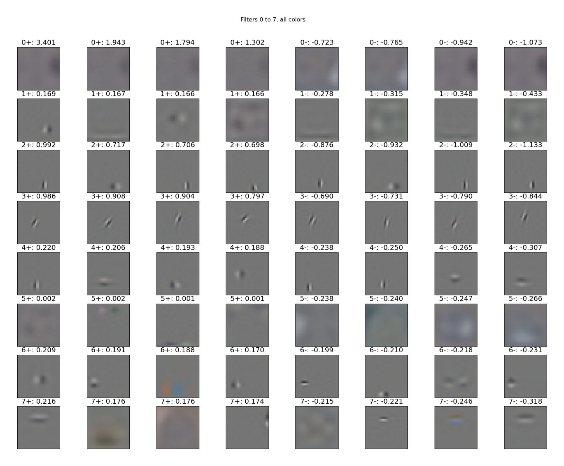
There is an intuitive way to interpret the weights of a Gaussian-Bernoulli RBM trained on images, and that is to look at the filters that the hidden units apply to the image. Each hidden unit is connected with some weight to each pixel. If we arrange these weights on a $32 \times 32$ grid, we obtain a visualization of the filter applied by the hidden unit. Figure 2.13 shows this type of visualization of 64 different hidden units. In creating these visualizations, we use intensity to indicate the strength of the weight. So a green region in the filter denotes a set of weights that have strong positive connections to the green channel of the pixels. But a purple region indicates strong negative connections to the green channel of the pixels, since this is the colour produced by setting the red and blue channels to high values and the green channel to a low value. In this sense, purple is "negative green," yellow is "negative blue," and turquoise is "negative red".

1.4.4 Measuring performance

Ideally, we would like to be able to evaluate $p(\mathbf{v})$ for data vector $\mathbf{v}$. But this is intractable for models with large numbers of hidden units due to the denominator in (1.3). Instead we use the "reconstruction error". The reconstruction error is the squared difference $(\mathbf{v} - \mathbf{v}')^2$ between the data vector $\mathbf{v}$, and the vector produced by sampling the hidden units given $\mathbf{v}$ to obtain a hidden configuration $\mathbf{h}$, and then sampling the visible units given $\mathbf{h}$ to obtain a visible configuration $\mathbf{v}'$. This is not a very good measure of how well the model's probability distribution matches that of the data, because the reconstruction error depends heavily on how fast the Markov chain mixes.

1.5 Feed-forward neural networks

In our experiments we use the weights learned by an RBM to initialize feed-forward neural networks which we train with the standard backpropagation algorithm. In Appendix B we give a brief overview of the algorithm.

Chapter 2: Learning a generative model of images

Section Summary: This chapter explores the quest to create a generative model for natural images that can identify useful high-level details, like the positions and directions of edges, to aid in classification tasks and mimic aspects of human vision. Early efforts, including previous studies and initial training on full images using a technique called an RBM, produced only random or useless patterns instead of meaningful features, even after attempts to filter out image noise by removing minor variations in the data. Success came when the researchers shifted to training smaller models on tiny 8x8 sections of images, which learned edge-detecting filters, and they combined these into a larger model for better results.

2.1 Motivation

The major, recurrent theme throughout this work is our search for a good generative model of natural images. In addition, we seek a model that is capable of extracting useful high-level features from images, such as the locations and orientations of contours. The hope is that such features would be much more useful to a classifier than the raw pixels. Finally, such a model would have some connection to the physical realities of human vision, as the visual cortex contains neurons that detect high-level features such as edges.

2.2 Previous work

One of the authors of the 80 million tiny images dataset unsuccessfully attempted to train the type of model that we are interested in here [3]. He was unsuccessful in the sense that the model he trained did not learn interesting filters. The model learned noisy global filters and point-like identity functions similar to the ones of Figure 2.12. Another group also attempted to train this type of model on $16 \times 16$ colour patches of natural images and came out only with filters that are everywhere uniform or global and noisy [7].

2.3 Initial attempts

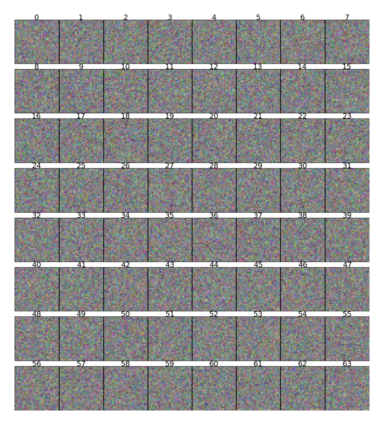
We started out by attempting to train an RBM with 8000 hidden units on a subset of 2 million images of the tiny images dataset. The subset was whitened but left otherwise unchanged. For this experiment we set the variance of each of the visible units to 1, since that is the variance that the whitening transformation produced. Unfortunately this model developed a lot of filters like the ones in Figure 2.1. Nothing that could be mistaken for a "feature".

2.4 Deleting directions of variance

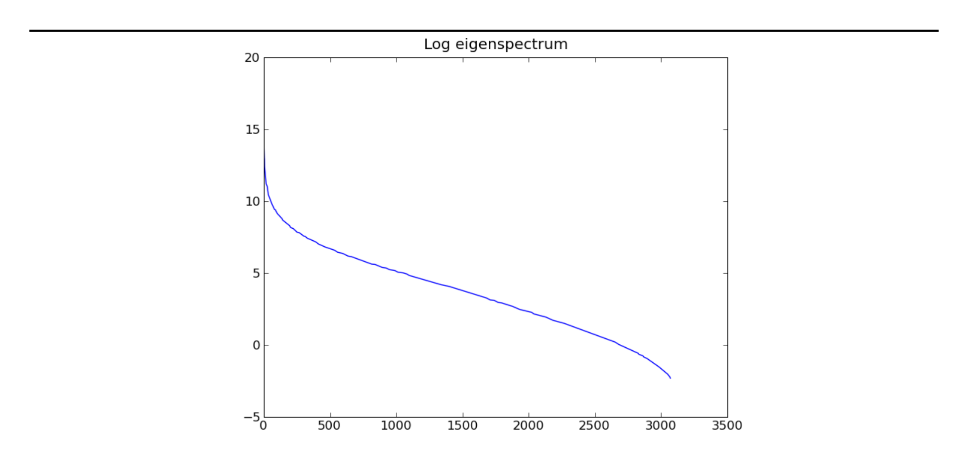
One theory was that high-frequency noise in the images was making it hard for the model to latch on to the real structure. It was busy modelling the noise, not the images. To mitigate this, we decided to remove some of the least significant directions of variance from the dataset. We accomplished this by setting to zero those entries of the diagonal matrix $D$ of equation (A.1) that correspond to the 1000 least significant principal components (these are the 1000 smallest entries of $D$). This has no discernible effect on the appearance of the images since the 2072 directions of variance that remain are far more important. In support of this claim, Figure 2.3 compares images that have been whitened and then dewhitened with the original filter with those using the new filter that also deletes the 1000 least significant principal components. Figure 2.2 plots the log-eigenspectrum of the tiny images dataset.

Unfortunately, this extra pre-processing step failed to convince the RBM to learn interesting features. But we nonetheless considered it a sensible step so we kept it for the remainder of our experiments.

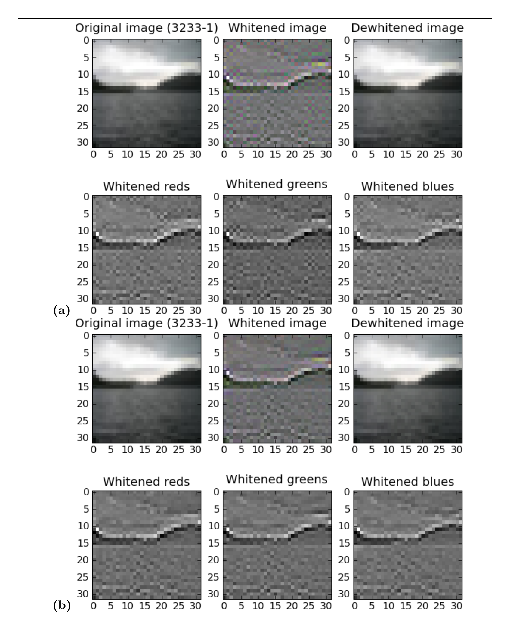
Notice that the whitened image appears smoother and less noisy in (b) than in (a), but the dewhitened image in (b) is identical to that in (a). This confirms that this modified whitening transformation is still invertible, even if not technically so.

2.5 Training on patches of images

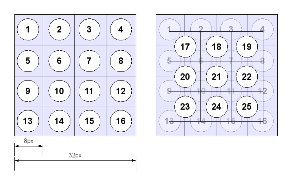
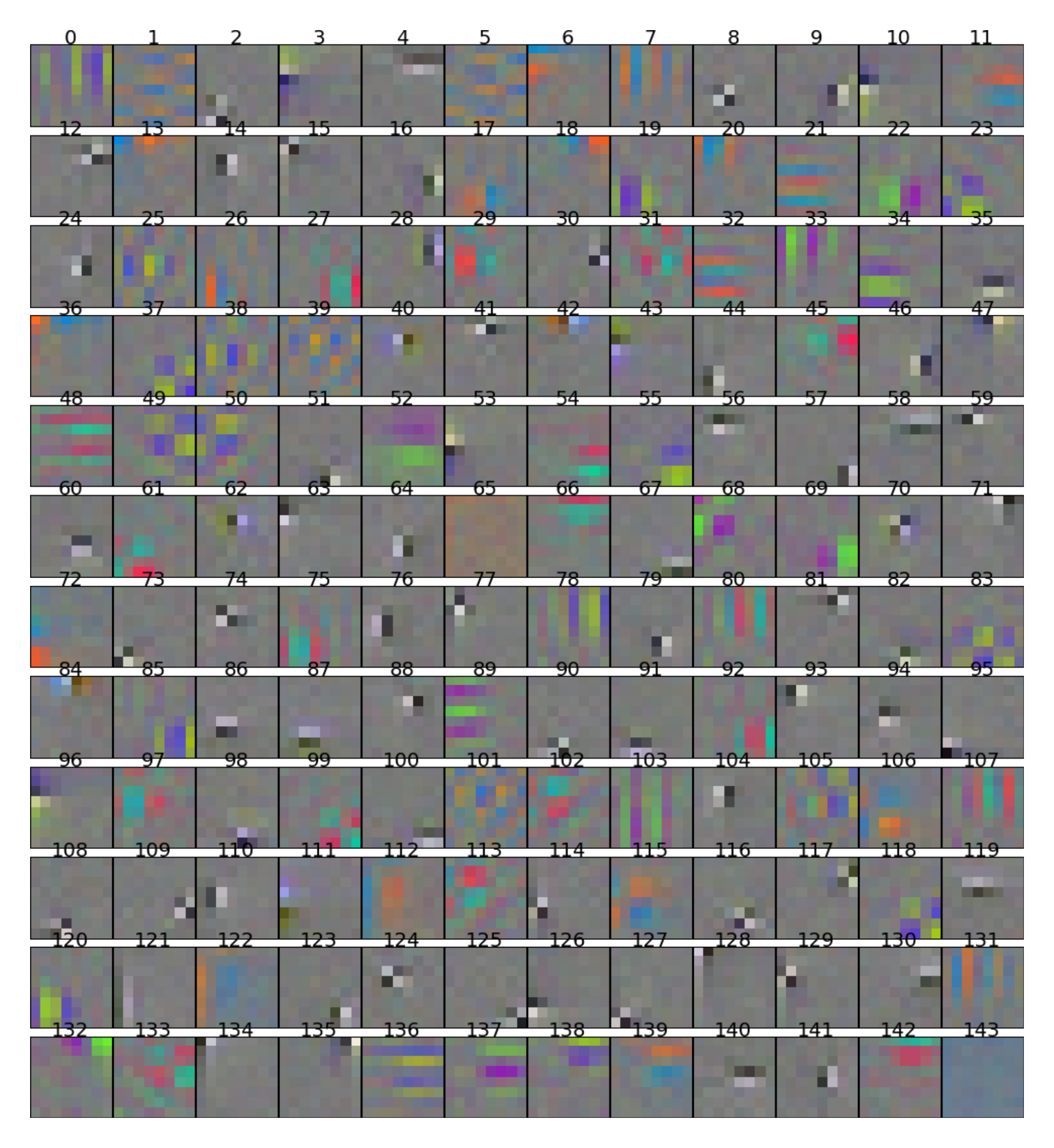
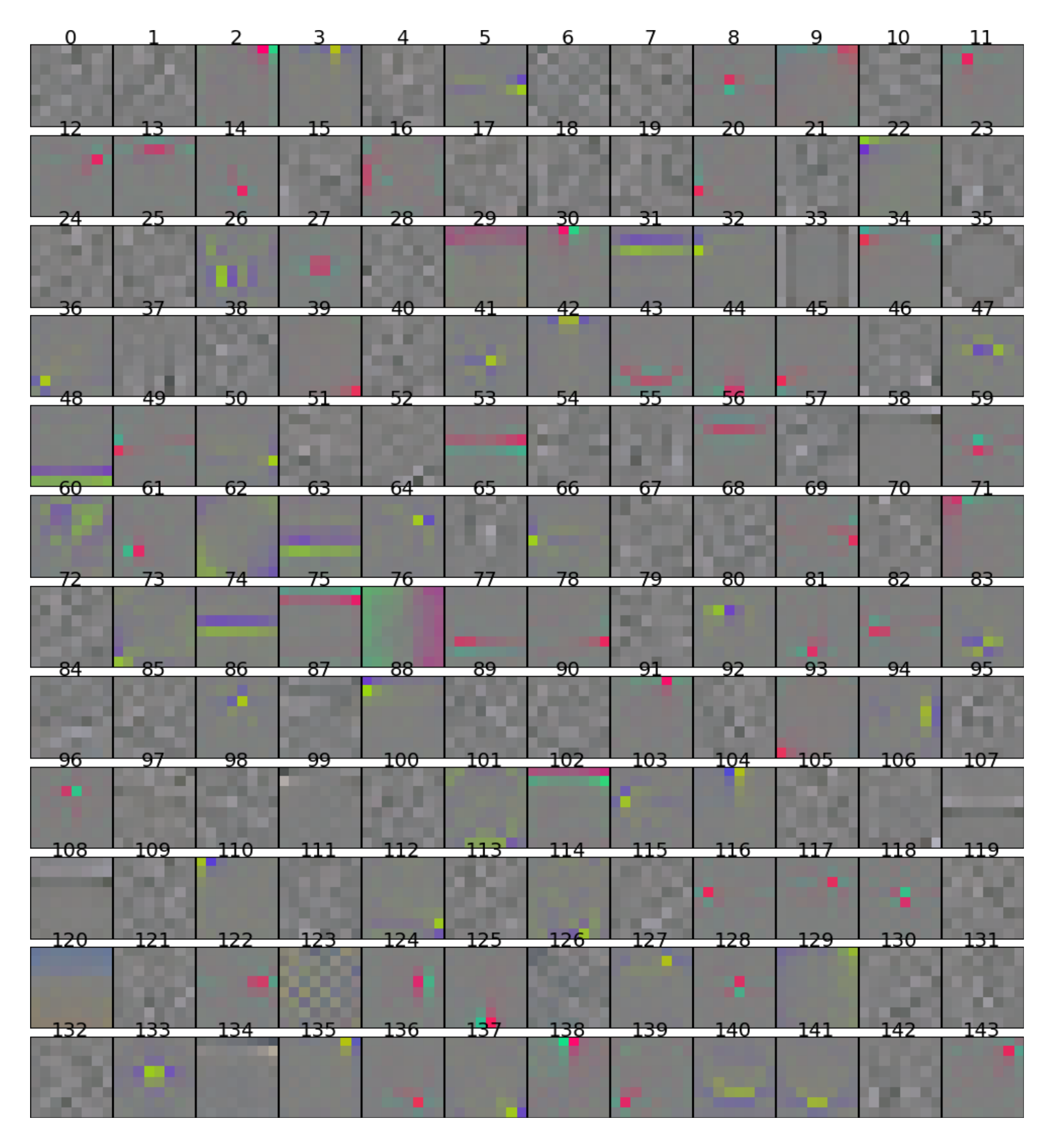
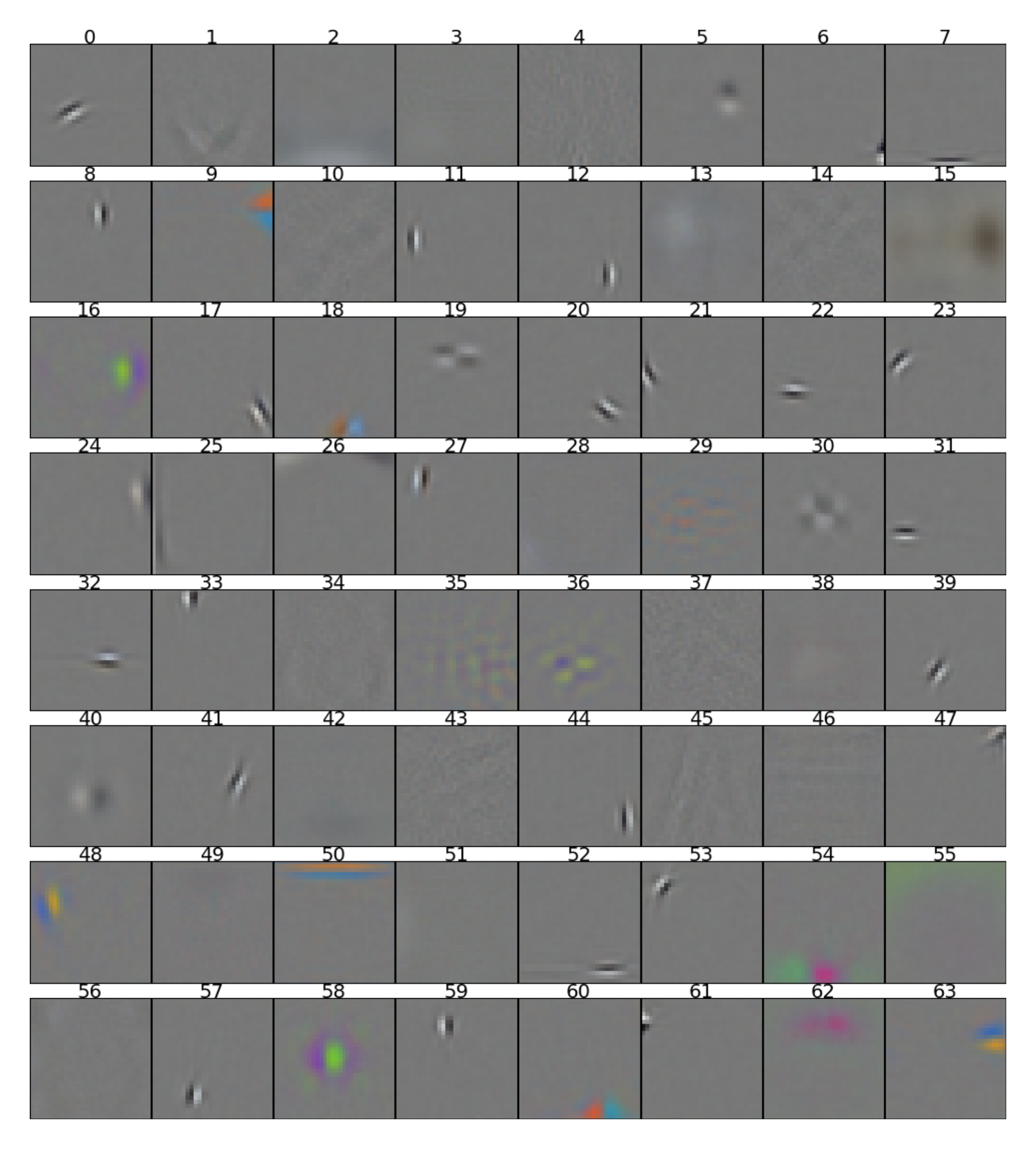
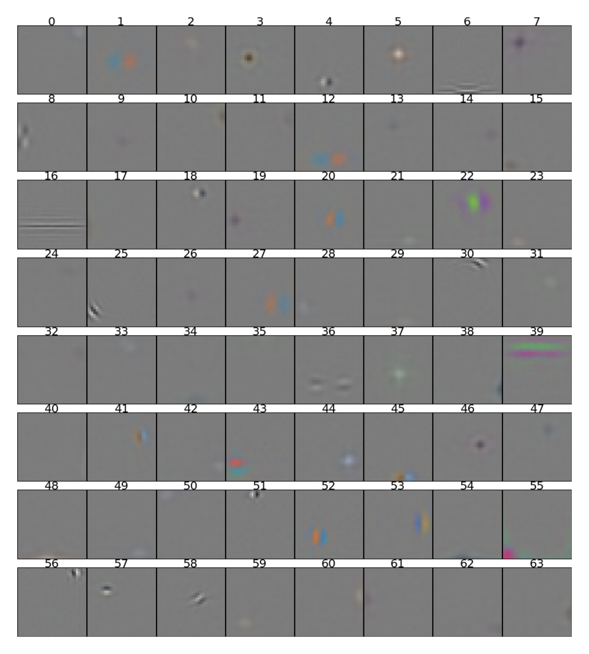
Frustrated by the model's inability to extract meaningful features, we decided to train on $8 \times 8$ patches of the images. This greatly reduced the data dimensionality and hence the required model complexity, measured in the number of hidden units. We divided the $32 \times 32$ images into 25 $8 \times 8$ patches as shown in Figure 2.4. In addition to the patches shown in Figure 2.4, we created a 26th patch: an $8 \times 8$ subsampled version of the entire $32 \times 32$ image. We trained 26 independent RBMs with 300 hidden units on each of these patches; Figures 2.5 and 2.6 show the filters that they learned. These are the types of filters that we were looking for — edge detectors.

One immediately noticeable pattern among the filters of Figure 2.5 is the RBM's affinity for low-frequency colour filters and high-frequency black-and-white filters. One explanation may be that the black-and-white filters are actually wider in the "colour dimension", since they have strong connections to all colour channels. We may also speculate that precise edge position information and rough colour information is sufficient to build a good model of natural images.

2.5.1 Merging RBMs trained on patches

Once we have trained 26 of these RBMs on the tiny image patches, we can combine them in a very straightforward (perhaps naive) way by training a new RBM with 7800 ($26 \times 300$) hidden units. We initialize the first 300 of these hidden units with the weights from the RBM trained on patch #1, the next 300 with the weights trained on patch #2, and so forth. However, each of the hidden units in the big RBM is connected to every pixel in the $32 \times 32$ image, so we initialize to 0 the weights that didn't exist in the RBMs trained on patches (for example, the weight from a pixel in patch #2 to a hidden unit from an RBM trained on patch #1). The weights from the hidden units that belonged to the RBM trained on patch #26 (the subsampled global patch) are initialized as depicted in Figure 2.7. The bias of a visible unit of the big RBM is initialized to the average bias that the unit received among the small RBMs.

Interestingly, this type of model behaves very well, in the sense that the weights don't blow up and the filters stay roughly as they were in the RBMs trained on patches. In addition, it is able to reconstruct images much better than the average small RBM is able to reconstruct image patches. This despite the fact that the patches that we trained on were overlapping, so the visible units in the big RBM must essentially learn to reconcile the inputs from two or three sets of hidden units, each of which comes from a different small RBM.

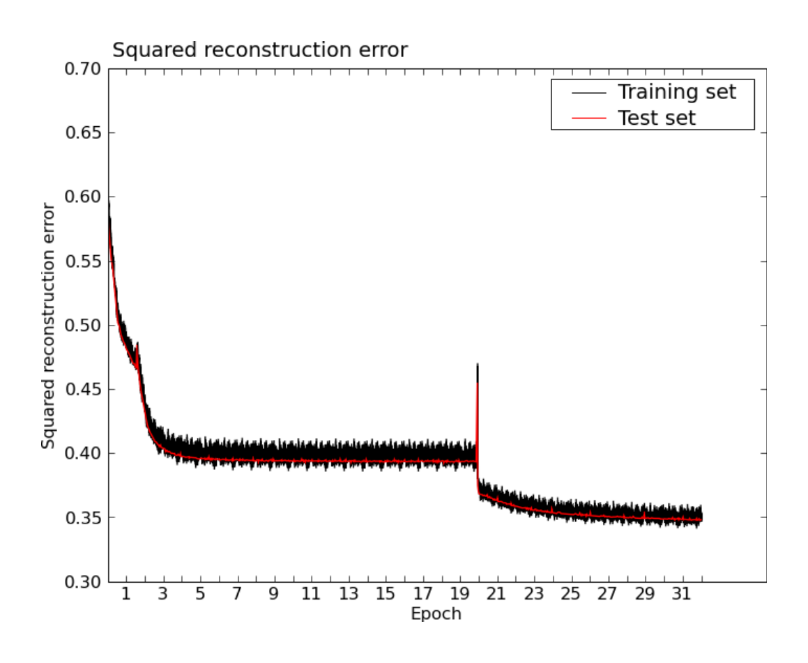
Figures 2.8 and 2.9 show some of the filters learned by this model (although in truth, they were for the most part learned by the small RBMs). Figure 2.10 shows the reconstruction error as a function of training time. The reconstruction error up to epoch 20 is the average among the independently-trained small RBMs. The large spike at epoch 20 is the point at which the small RBMs were combined into one big RBM. The merger initially has an adverse effect on the reconstruction error but it very quickly descends below its previous minimum.

2.6 Training RBMs on 32x32 images

After our successes training models of $8 \times 8$ and $16 \times 16$ patches, we decided to try with $32 \times 32$ images once more. This time we developed an algorithm for parallelizing the training across all the CPU cores of a machine. Later, we further parallelized across machines on a network, and this algorithm is described in Chapter 4.

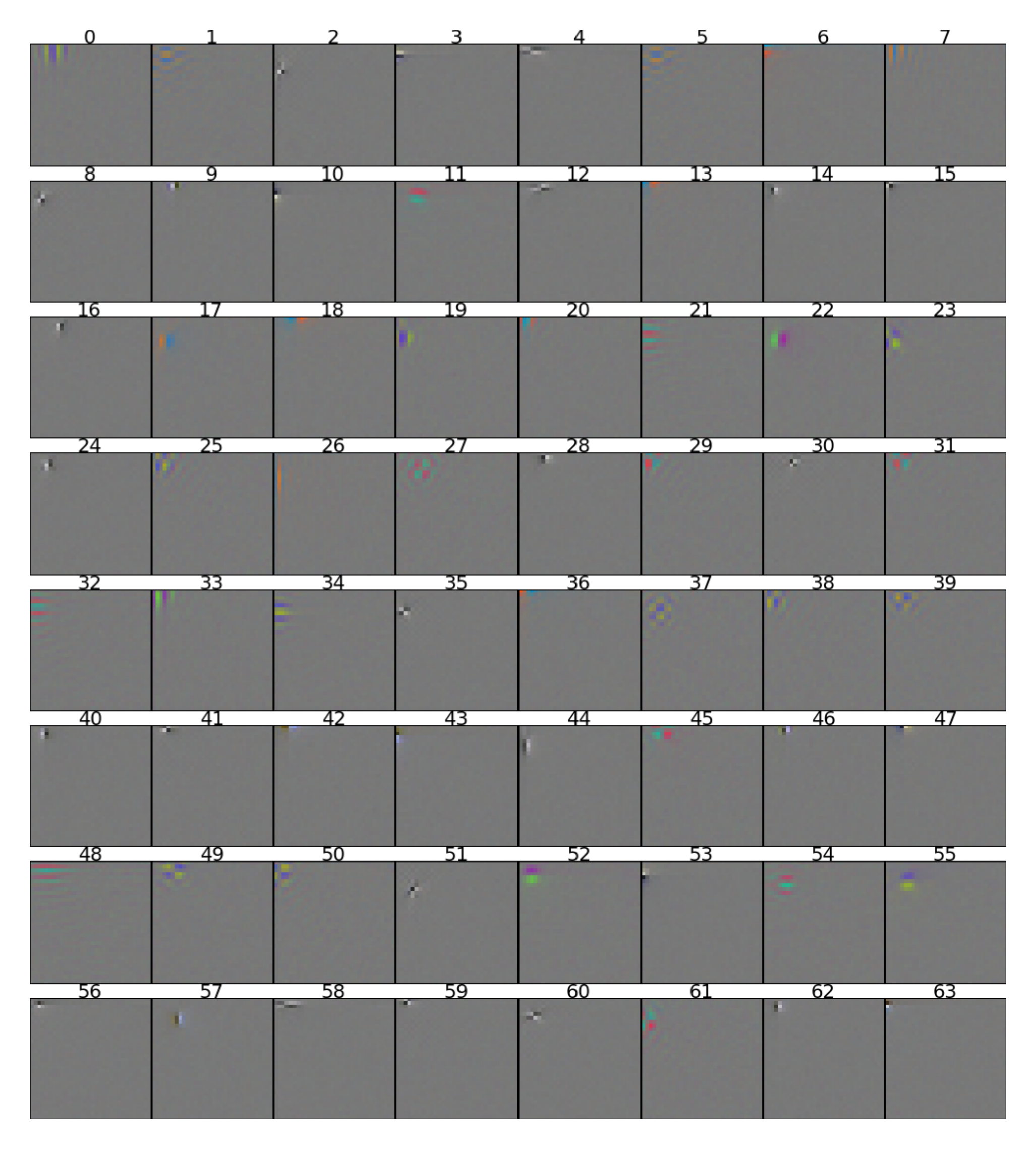
With this new, faster training algorithm we were quickly able to train an RBM with 10000 hidden units on the $32 \times 32$ whitened images. A sample of the filters that it learned is shown in Figure 2.11. They appear very similar to the filters learned by the RBMs trained on patches.

After successfully training this RBM, we decided to try training an RBM on unwhitened data. We again preprocessed the data by deleting the 1000 least-significant directions of variance, as described in section 2.4. We measured the average standard deviation of the pixels in this dataset to be 69, so we set the standard deviation of the visible units of the RBM to 69 as well. A curious thing happens when training on unwhitened data – all of the filters go through a point stage before they turn into edge filters. A sample of such point filters is shown in Figure 2.12. In the point stage, the filters simply "copy" data from the visible units to the hidden units. The filters remain in this point stage for a significant amount of time, which can create the illusion that the RBM has finished learning and that further training is futile. However, the point filters eventually evaporate and in their place form all kinds of edge filters, a sample of which is shown in Figure 2.13[^1]. The edge filters do not necessarily form at or near the positions of their pointy ancestors, though this is common. Notice that these filters are generally larger than the ones learned by the RBM trained on whitened data (Figure 2.11). This is most likely due to the fact that a green pixel in a whitened image can indicate a whole region of green in the unwhitened image.

[^1]: Note that these filters are from a different RBM than that which produced the point filters pictured in Figure 2.12.

2.7 Learning visible standard deviations

We then turned our attention to learning the standard deviations of the visible units. Notice that the edge filters learned by this RBM have a higher frequency than those learned by the RBM of Figure 2.13. This is due to the fact that this RBM has learned to set its visible standard deviations to values lower than 1, and so its hidden units learned to be more precise.](figure_028_page30.png)

Every row represents a hidden unit $h$ in the second-level RBM, and in every column are the filters of the first-level RBM to which $h$ has the strongest connections. The four filters on the left are the ones to which $h$ has the strongest positive connection and the four filters on the right are the ones to which $h$ has the strongest negative connections.

In a few instances we see examples of the RBM favouring a certain edge filter orientation and disfavouring the mirror orientation (see for example second-last row, columns 2 and 8).

Chapter 3: Object classification experiments

Section Summary: Researchers created the CIFAR-10 dataset by hiring students to carefully label and clean 60,000 images from a larger collection, focusing on ten everyday object classes like airplanes, cars, and animals, ensuring each image showed a single, clear, realistic example. They also developed a related CIFAR-100 dataset with more classes for added complexity. To classify these images, they tested various computer models, finding that ones using learned features from specialized algorithms called RBMs outperformed simple pixel-based approaches, with a neural network fine-tuned from these features achieving the best accuracy.

3.1 The labeled subset[^1]

We paid students to label a subset of the tiny images dataset. The labeled subset we collected consists of ten classes of objects with 6000 images in each class. The classes are airplane, automobile (but not truck or pickup truck), bird, cat, deer, dog, frog, horse, ship, and truck (but not pickup truck). Since each image in the dataset already comes with a noisy label (the search term used to find the image), all we needed the labelers to do was to filter out the mislabeled images. To that end, each labeler was given a class and asked to examine all the images which were found with that class as the search term. Since the dataset contains only about 3000 images per search term, the labelers were also asked to examine all the images which were found with a search term that is a hyponym (as defined by WordNet) of the main search term. As an example, some of the hyponyms of ship are cargo ship, ocean liner, and frigate. The labelers were instructed to reject images which did not belong to their assigned class. The criteria for deciding whether an image belongs to a class were as follows[^2]:

• The class name should be high on the list of likely answers to the question "What is in this picture?"
• The image should be photo-realistic. Labelers were instructed to reject line drawings.
• The image should contain only one prominent instance of the object to which the class refers.
• The object may be partially occluded or seen from an unusual viewpoint as long as its identity is still clear to the labeler.

The labelers were paid a fixed sum per hour spent labeling, so there was no incentive to rush through the task. Furthermore, we personally verified every label submitted by the labelers. We removed duplicate images from the dataset by comparing images with the L2 norm and using a rejection threshold liberal enough to capture not just perfect duplicates but also re-saved JPEGs and the like. Finally, we divided the dataset into a training and test set, the training set receiving a randomly-selected 5000 images from each class.

We call this the CIFAR-10 dataset, after the Canadian Institute for Advanced Research, which funded the project. In addition to this dataset, we have labeled another set – 600 images in each of 100 classes. This we call the CIFAR-100 dataset. The methodology for collecting this dataset was identical to that for CIFAR-10. The CIFAR-100 classes are mutually exclusive with the CIFAR-10 classes, and so they can be used as negative examples for CIFAR-10. For example, CIFAR-10 has the classes automobile and truck, but neither of these classes includes images of pickup trucks. CIFAR-100 has the class pickup truck. Furthermore, the CIFAR-100 classes come in 20 superclasses of five classes each. For example, the superclass reptile consists of the five classes crocodile, dinosaur, lizard, turtle, and snake. The idea is that classes within the same superclass are similar and thus harder to distinguish than classes that belong to different superclasses. Appendix D lists the entire class structure of CIFAR-100.

All of our experiments were with the CIFAR-10 dataset because the CIFAR-100 was only very recently completed.

[^1]: We thank Vinod Nair for his substantial contribution to the labeling project.

[^2]: The instruction sheet which was handed out to the labelers is reproduced in Appendix C.

3.2 Methods

We compared several methods of classifying the images in the CIFAR-10 dataset. Each of these methods used multinomial logistic regression at its output layer, so we distinguish the methods mainly by the input they took:

1. The raw pixels (unwhitened).
2. The raw pixels (whitened).
3. The features learned by an RBM trained on the raw pixels.
4. The features learned by an RBM trained on the features learned by the RBM of #3.

One can also use the features learned by an RBM to initialize a neural network, and this gave us our best results (this approach was presented in [6]). The neural net had one hidden layer of logistic units ($f(x) = \frac{1}{1+e^{-x}}$), whose weights to the visible units we initialized from the RBM trained on raw (unwhitened) pixels. We initialized the hidden-to-output weights from the logistic regression model trained on RBM features as input. So, initially, the output of the neural net was exactly identical to the output of the logistic regression model. But the net learned to fine-tune the RBM weights to improve generalization performance slightly. In this fashion it is also possible to initialize two-hidden-layer neural nets with the features learned by two layers of RBMs, and so forth. However, two hidden layers did not give us any improvement over one. This result is in line with that found in [10].

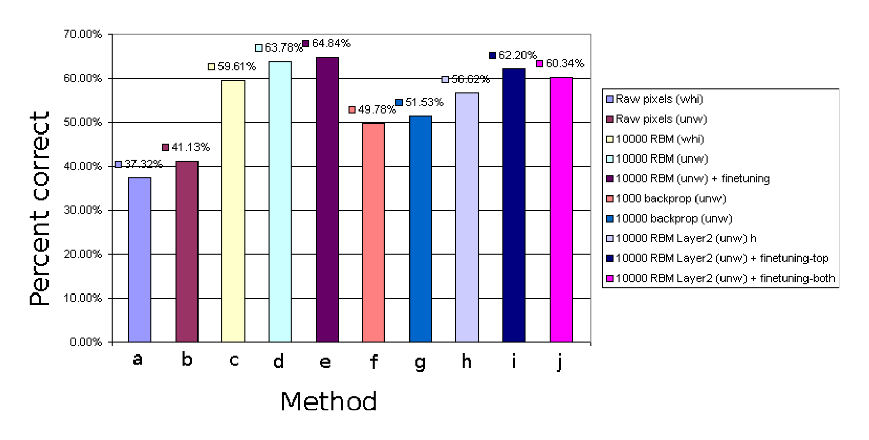
Our results are summarized in Figure 3.1[^3]. Each of our models produced a probability distribution over the ten classes, so we took the most probable class as the model's prediction. We found that the RBM features were far more useful in the classification task than the raw pixels. Furthermore, features from an RBM trained on unwhitened data outperformed those from an RBM trained on whitened data. This may be due to the fact that the whitening transformation fixes the variance in every direction at 1, possibly exaggerating the significance of some directions which correspond mainly to noise (although, as mentioned, we deleted the 1000 least-significant directions of variance from the data). The neural net that was initialized with RBM features achieved the best result, just slightly improving on the logistic regression model trained on RBM features. The figure also makes clear that, for the purpose of classification, the features learned by an RBM trained on the raw pixels are superior to the features learned by a randomly-initialized neural net. We should also mention that the neural nets initialized from RBM features take many fewer epochs to train than the equivalently-sized randomly-initialized nets, because all the RBM-initialized neural net has to do is fine-tune the weights learned by the RBM which was trained on 2 million tiny images[^4].

[^3]: The last model performed slightly worse than the second-last model probably because it had roughly $2 \times 10^8$ parameters and thus had a strong tendency to overfit. The model's size also made it slow and very cumbersome to train. We did not run many instances of it to find the best setting of the hyperparameters.

[^4]: Which, admittedly, it took a long time to learn.

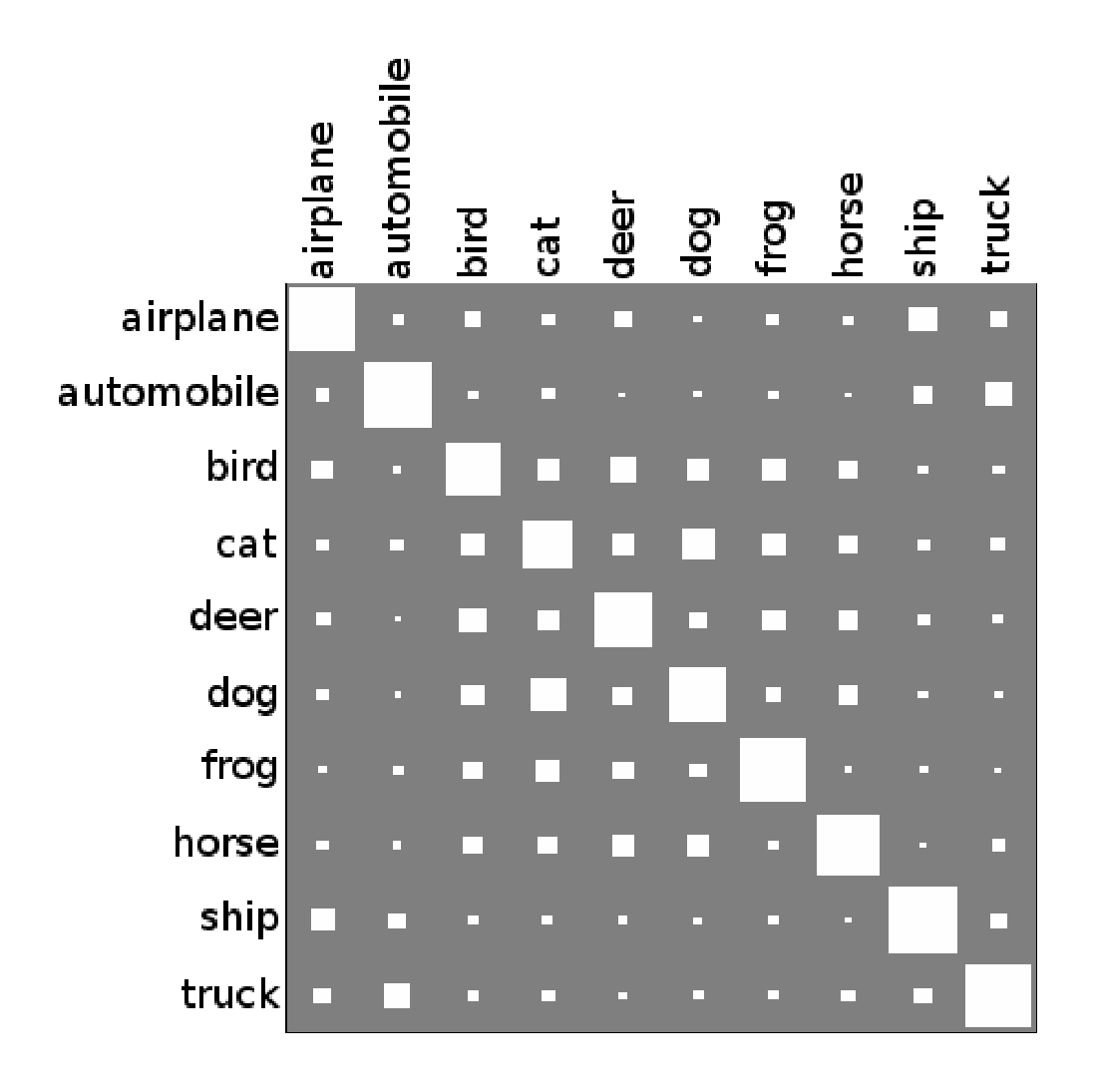
Figure 3.2 shows the "confusion matrix" of the logistic regression model trained on RBM features (unwhitened). The matrix summarizes which classes get mistaken for which other classes by the model. It is interesting to note that the animal classes seem to form a distinct cluster from the non-animal classes. Seldom is an animal mistaken for a non-animal, save for the occasional misidentification of a bird as a plane[^5].

[^5]: It is a pity we did not have the foresight to include Superman as the 11th class.

(a,b) Logistic regression on the raw, whitened and unwhitened data. (c,d) Logistic regression on 10000 RBM features from an RBM trained on whitened, unwhitened data. (e) Backprop net with one hidden layer initialized from the 10000 features learned by an RBM trained on unwhitened data. The hidden-out connections were initialized from the model of (d). (f) Backprop net with one hidden layer of 1000 units, trained on unwhitened data and with logistic regression at the output. (g) Backprop net with one hidden layer of 10000 units, trained on unwhitened pixels and with logistic regression at the output. (h) Logistic regression on 10000 RBM features from an RBM trained on the 10000 features learned by an RBM trained on unwhitened data. (i) Backprop net with one hidden layer initialized from the 10000 features learned by an RBM trained on the 10000 features from an RBM trained on unwhitened data. The hidden-out connections were initialized from the model of (h). (j) Backprop net with two hidden layers, the first initialized as in (e) and the second as in (i). The hidden-out connections were initialized as in (i) as well.

Notice how frequently a cat is mistaken for a dog, and how infrequently an animal is mistaken for a non-animal (or vice versa).

Chapter 4: Parallelizing the training of RBMs

Section Summary: This chapter outlines a method for speeding up the training of restricted Boltzmann machines (RBMs), a type of neural network, by distributing the workload across multiple computers. The approach divides the network's hidden and visible components among the machines, allowing each to perform partial calculations on the data before sharing results to synchronize and complete the updates, based on a technique called contrastive divergence. It works especially well for networks with binary data, requiring minimal communication that grows steadily with more machines, and can even use multiple processor cores on each computer for further efficiency.

4.1 Introduction

Here we describe an algorithm for parallelizing the training of RBMs. When both the hidden and visible units are binary, the algorithm is extremely efficient, in that it requires very little communication and hence scales very well. When the visible units are Gaussian the algorithm is less efficient but in the problem we tested, it scales nearly as well as in the binary-to-binary case. In either case the total amount of communication required scales linearly with the number of machines, while the amount of communication required per machine is constant. If the machines have more than one core, the work can be further distributed among the cores. The specific algorithm we will describe is a distributed version of CD-1, but the principle remains the same for any variant of CD, including Persistent CD (PCD)[13].

4.2 The algorithm

Recall that (undistributed) CD-1 training consists roughly of the following steps, where there are $I$ visible units and $J$ hidden units:

1. Get the data $V = [v_0, v_1, ..., v_I]$.
2. Compute hidden unit activities $H = [h_0, h_1, ..., h_J]$ given the data.
3. Compute visible unit activities ("negative data") $V' = [v'_0, v'_1, ..., v'_I]$ given the hidden unit activities of the previous step.
4. Compute hidden unit activities $H' = [h'_0, h'_1, ..., h'_J]$ given the visible unit activities of the previous step.

The weight update for weight $w_{ij}$ is

$ \Delta w_{ij} = \epsilon (v_i h_j - v'_i h'_j). $

If we're doing batch training, the weight update is

$ \Delta w_{ij} = \epsilon (\langle v_i h_j \rangle - \langle v'_i h'_j \rangle) $

where $\langle \rangle$ denotes expectation among the training cases in the batch.

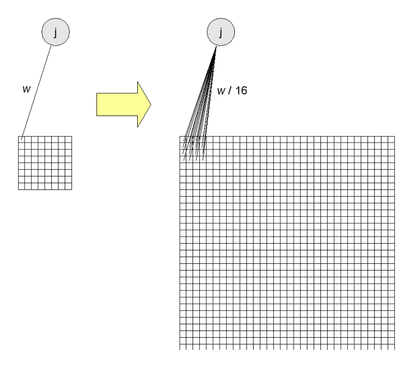
The distributed algorithm parallelizes steps 2, 3, and 4 and inserts synchronization points[^6] after each of these steps so that all the machines proceed in lockstep. If there are $n$ machines, each machine is responsible for computing $1/n$ of the hidden unit activities in steps 2 and 4 and $1/n$ of the visible unit activities in step 3. We assume that all machines have access to the whole dataset. It's probably easiest to describe this with a picture. Figure 4.1 shows which weights each machine "cares about" (i.e. which weights it has to know) when there are four machines in total.

[^6]: A synchronization point is a section of code that all machines must execute before any machine can proceed beyond it.

For $K$ machines, the algorithm proceeds as follows:

1. Each machine has access to the whole dataset so it knows $V = [v_0, v_1, ..., v_I]$.
2. Each machine $k$ computes its hidden unit activities $H_k = [h^k_0, h^k_1, ..., h^k_{J/K}]$ given the data $V$. Note that each machine computes the hidden unit activities of only $J/K$ hidden units. It does this using the green weights in Figure 4.1.
3. All the machines send the result of their computation in step 2 to each other.
4. Now knowing all the hidden unit activities, each machine computes its visible unit activities ("negative data") $V'k = [v'^k_0, v'^k_1, ..., v'^k{I/K}]$ using the purple weights in Figure 4.1.
5. All the machines send the result of their computation in step 4 to each other.
6. Now knowing all the negative data, each machine computes its hidden unit activities $H'k = [h'^k_0, h'^k_1, ..., h'^k{J/K}]$ using the green weights in Figure 4.1.
7. All the machines send the result of their computation in step 6 to each other.

Notice that since each $h_j$ is only 1 bit, the cost of communicating the hidden unit activities is very small. If the visible units are also binary, the cost of communicating the $v_i$s is also small. This is why the algorithm scales particularly well for binary-to-binary RBMs.

After step 3, each machine has enough data to compute $\langle v_i h_j \rangle$ for all the weights that it cares about. After step 7, each machine has enough data to compute $\langle v'_i h'_j \rangle$ for all the weights that it cares about. This is essentially all there is to it.

You'll notice that most weights are updated twice (but on different machines), because most weights are known to two machines (in Figure 4.1 notice, for example, that some green weights on machine 1 are purple weights on machine 2). This is the price of parallelization. In fact, in our implementation, we updated every weight twice, even the ones that are known to only one machine. This is a relatively small amount of extra computation, and avoiding it would result in having to do two small matrix multiplications instead of one large one.

Wary of floating point nastiness, you might also wonder: if each weight update is computed twice, can we be sure that the two computations arrive at exactly the same answer? When the visible units are binary, we can. This is because the "floating point operations" constitute taking the product of the data matrix with the matrix of hidden activities, both of which are binary (although they are likely to be stored as floating point). When the visible units are Gaussian, however, this really does present a problem. Because we have no control over the matrix multiplication algorithm that our numerical package uses to compute matrix products, and further because each weight may be stored in a different location of the weight matrix on each machine (and the weight matrices may even have slightly different shapes on different machines!), we cannot be sure that the sequence of floating point operations that compute weight update $\Delta w_{ij}$ on one machine will be exactly the same as that which compute it on a different machine. This causes the values stored for these weights to diverge on the two machines and requires that we introduce a weight synchronization step to our algorithm. In practice, the divergence is very small even if all our calculations are done in single-precision floating point, so the weight synchronization step need not execute very frequently. The weight synchronization step proceeds as follows:

1. Designate the purple weights (Figure 4.1) as the weights of the RBM and forget about the green weights.
2. Each machine $k$ sends to machine $k'$ the slice of its purple weights that machine $k'$ needs to know in order to fill in its green weights.

Notice that each machine must send $\frac{1}{K}$th of the weight matrix to $K-1$ machines. Since $K$ machines are sending stuff around, the total amount of communication does not exceed $\frac{K-1}{K} \cdot (\text{size of weight matrix})$. Thus the amount of communication required for weight synchronization is constant in the number of machines, which means that floating point does not manage to spoil the algorithm – the algorithm does not require an inordinate amount of correction as the number of machines increases.

We've omitted biases from our discussion thus far; that is because they are only a minor nuisance. The biases are divided into $K$ chunks just like the weights. Each machine is responsible for updating the visible biases corresponding to the visible units on the purple weights in Figure 4.1 and the hidden biases corresponding to the hidden units on the green weights in Figure 4.1. Each bias is known to only one machine, so its update only has to be computed once. Recall that the bias updates in CD-1 are

$ \Delta b^v_i = \epsilon (\langle v_i \rangle - \langle v'_i \rangle), $

$ \Delta b^h_j = \epsilon (\langle h_j \rangle - \langle h'_j \rangle) $

where $b^v_i$ denotes the bias of visible unit $i$ and $b^h_j$ denotes the bias of hidden unit $j$. Clearly after step 1, each machine can compute $\langle v_i \rangle$. After step 2 it can compute $\langle h_j \rangle$. After step 4 it can compute $\langle v'_i \rangle$. And after step 6 it can compute $\langle h'_j \rangle$.

4.3 Implementation

We implemented this algorithm as a C extension to a Python program. The Python code initializes the matrices, communication channels, and so forth. The C code does the actual computation. We use whatever implementation of BLAS (Basic Linear Algebra Subprograms) is available to perform matrix and vector operations.

We use TCP sockets to communicate between machines. Our implementation is also capable of distributing the work across multiple cores of the same machine, in the same manner as described above. The only difference is that communication between cores is done via shared memory instead of sockets. We used the pthreads library to parallelize across cores.

We execute the weight synchronization step after training on each batch of 8000 images. This proved sufficient to keep the weights synchronized to within $10^{-9}$ at single precision. Our implementation also computes momentum and weight decay for all the weights.

When parallelizing across $K$ machines, our implementation spawns $K-1$ writer threads and $K-1$ reader threads on each machine, in addition to the threads that do the actual computation (the "worker" threads). The number of worker threads is a run-time variable, but it is most sensible to set it to the number of available cores on the machine.

4.3.1 Writer threads

Each writer thread is responsible for sending data to a particular other machine. Associated with each writer thread is a queue. The worker threads add items to these queues when they have finished their computation. The writer threads dequeue these items and send them to their target machine. We have separated communication from computation in this way so that a machine that has everything it needs to continue its computation does not need to delay performing it just because it still has to send some data to another machine.

4.3.2 Reader threads

Each reader thread is responsible for receiving data from a particular other machine. The reader thread reads data from its target machine as soon as it arrives. This setup ensures that no attempt to send data ever blocks because the receiver is still computing. There is always a thread on the other side that's ready to receive. Similarly, since the data is received as soon as it becomes available, no machine ever has to delay receiving data merely because it is still computing.

4.4 Results

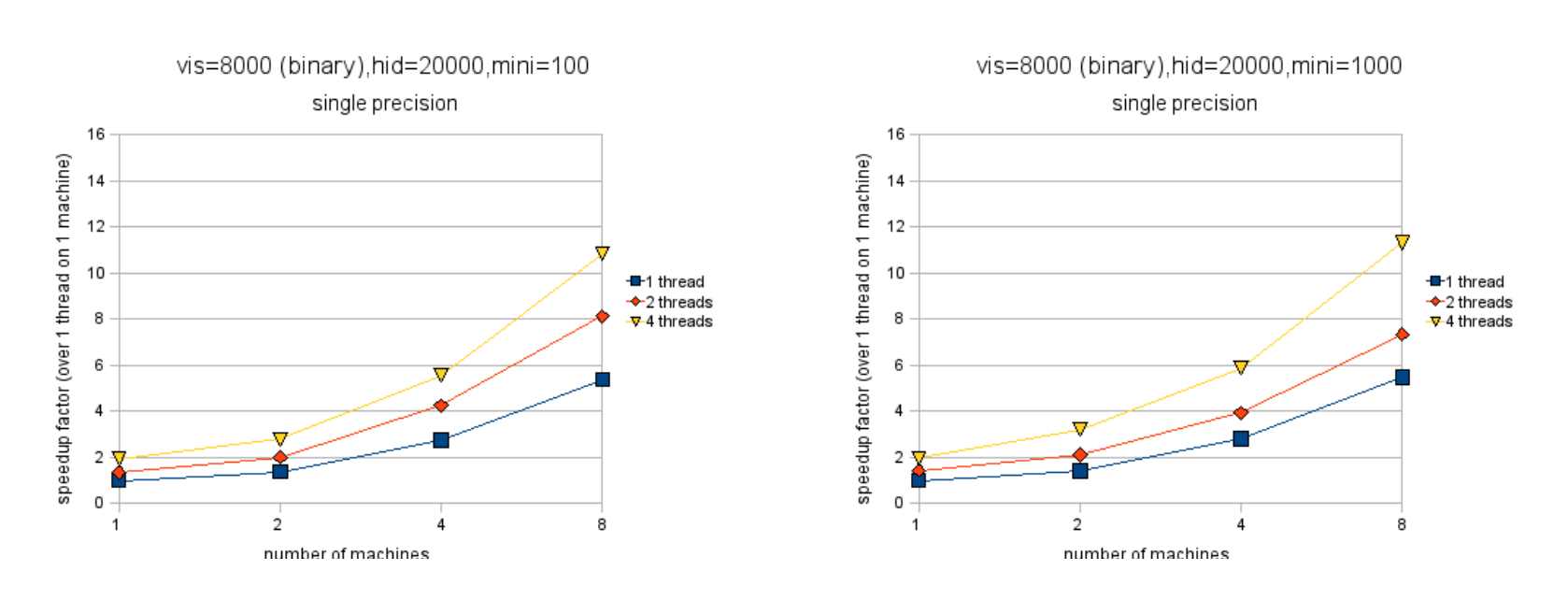
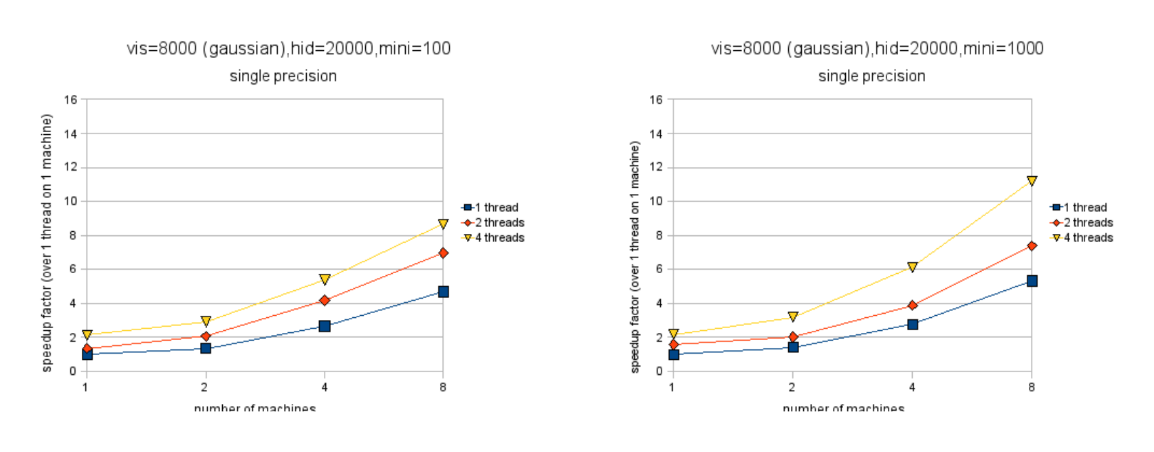
We have tested our implementation of the algorithm on a relatively large problem – 8000 visible units and 20000 hidden units. The training data consisted of 8000 examples of random binary data (hopefully no confusion arises from the fact that we have two different quantities whose value is 8000). We ran these tests on machines with two dual-core Intel Xeon 3GHz CPUs. We used Intel's MKL (Math Kernel Library) for matrix operations. These machines are memory bandwidth-limited so returns diminished when we started running the fourth thread. We measured our network speed at 105 MB/s, where 1 MB = 1000000 bytes. We measured our network latency at 0.091ms. Our network is such that multiple machines can communicate at the peak speed without slowing each other down. In all our experiments, the weight synchronization step took no more than four seconds to perform (two seconds at single precision), and these times are included in all our figures. The RBM we study here takes, at best, several minutes per batch to train (see Figure 4.4), so the four-second synchronization step is imperceptible.

Figures 4.2 and 4.3 show the speedup factor when parallelizing across different numbers of machines and threads[^7]. Note that these figures do not show absolute speeds so no comparison between them (nor between the subfigures) is possible. Figures 4.4 and 4.5 show the actual computation times of these RBMs on 8000 training examples. Not surprisingly, double precision is slower than single precision and smaller minibatch sizes are slower than larger ones. Single precision is much faster initially (nearly 3x) but winds up about 2x faster after much parallelization.

[^7]: The numbers for one thread running on one machine were computed using a different version of the code – one that did not incur all the overhead of parallelization. The numbers for multiple threads running on one machine were computed using yet a third version of the code – one that did not incur the penalty of parallelizing across machines (i.e. having to compute each weight update twice). When parallelizing merely across cores and not machines, there is a variant of this algorithm in which each weight only has to be updated once and only by one core, and all the other cores immediately "see" the new weight after it has been updated. This variant also reduces the number of sync points from three to two per iteration.

There are a couple of other things worth noting. For binary-to-binary RBMs, it is in some cases better to parallelize across machines than across cores. This effect is impossible to find with Gaussian-to-binary RBMs, the cost of communication between machines making itself shown. The effect is also harder to find for binary-to-binary RBMs when the minibatch size is 100, following the intuition that the efficiency of the algorithm will depend on how frequently the machines have to talk to each other. The figures also make clear that the algorithm scales better when using double-precision floating point as opposed to single-precision, although single-precision is still faster in all cases.

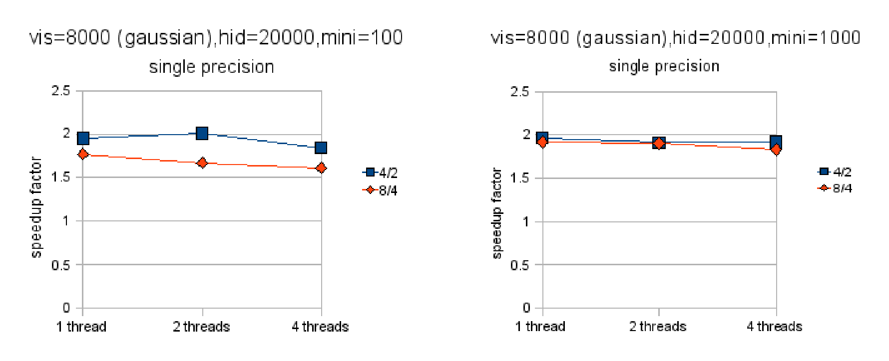
With binary visible units, the algorithm appears to scale rather linearly with the number of machines. Figure 4.6 illustrates this vividly. It shows that doubling the number of machines very nearly doubles the performance in all cases[^8]. This suggests that the cost of communication is negligible, even in the cases when the minibatch size is 100 and the communication is hence rather fragmented. When the visible units are Gaussian, the algorithm scales just slightly worse. Notice that when the minibatch size is 1000,

[^8]: The reason we didn't show the speedup factor when using two machines versus one machine on these graphs is that the one-machine numbers were computed using different code (explained in the previous footnote) and so they wouldn't offer a fair comparison.

![Figure 4.3: Speedup due to parallelization for a Gaussian-to-binary RBM (versus one thread running on one machine). (a) Minibatch size 100, double precision floats, (b) minibatch size 1000, double precision floats, (c) minibatch size 100, single precision floats, (d) minibatch size 1000, single precision floats.

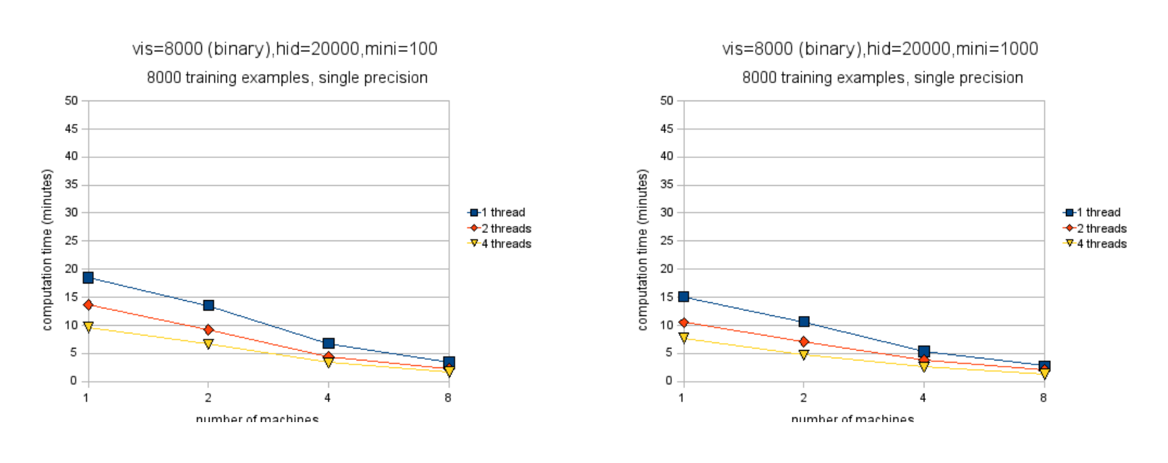
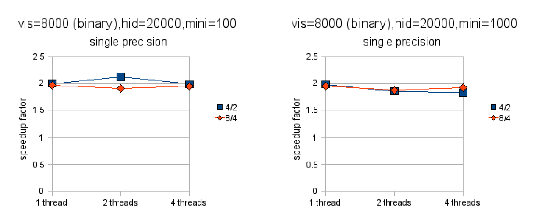
the algorithm scales almost as well in the Gaussian-to-binary case as in the binary-to-binary case. When the minibatch size is 100, the binary-to-binary version scales better than the Gaussian-to-binary one. Figure 4.7 shows that in the Gaussian-to-binary case doubling the number machines almost, but not quite, doubles performance.

4.4.1 Communication cost analysis

We can analyze the communication cost more formally. Given $K$ machines, we can compute the amount of data transmitted per training batch of 8000 examples like this: in steps 3 and 7, each machine has to send its hidden unit activities to all the other machines. Thus it has to send

$ 2 \cdot (K - 1) \cdot 8000 \cdot \frac{20000}{K} \text{ bits}. $

In step 5 each machine has to send its visible unit activities to all the other machines. If the visible units are binary, this is another

$ (K - 1) \cdot 8000 \cdot \frac{8000}{K} \text{ bits}. $

These sum to

$ \frac{(K - 1) (3.84 \times 10^8)}{K} \text{ bits} $

$ = 48 \cdot \frac{(K - 1)}{K} \text{ MB}. $

Thus the total amount of data sent (equivalently, received) by all machines is $48 \cdot (K - 1)$ MB. In the Gaussian-to-binary case, this number is appropriately larger depending on whether we're using single or double precision floats. In either case, the cost of communication rises linearly with the number of machines. Table 4.1 shows how much data was transferred by the RBMs that we trained (not including weight synchronization, which is very quick). Note that the cost of communication per machine is bounded from above by a constant (48MB in this case). So if machines can communicate with each other without slowing down the communication of other machines, the communication cost essentially does not increase with the number of machines.

: Table 4.1: Total amount of data sent (equivalently, received) by the RBMs discussed in the text.

\begin{tabular}{|c|c|c|c|c|}
\hline
\textbf{Number of machines:} & 1 & 2 & 4 & 8 \\ \hline
\textbf{Data sent (MB) (binary visibles):} & 0 & 48 & 144 & 336 \\ \hline
\textbf{Data sent (MB) (Gaussian visibles, single precision):} & 0 & 296 & 888 & 2072 \\ \hline
\textbf{Data sent (MB) (Gaussian visibles, double precision):} & 0 & 552 & 1656 & 3864 \\ \hline
\end{tabular}

It looks as though we have not yet reached the point at which the benefit of parallelization is outweighed by the cost of communication for this large problem. But when we used this algorithm to train an RBM on binarized MNIST digits (784 visible units, 392 hidden units), the benefits of parallelization disappeared after we added the second machine. But at that point it was already taking only a few seconds per batch.

4.5 Other algorithms

We'll briefly discuss a few other algorithms that could be used to parallelize RBM training. All of these algorithms require a substantial amount of inter-machine communication, so they are not ideal for binary-to-binary RBMs. But for some problems, some of these algorithms require less communication in the Gaussian-to-binary case than does the algorithm we have presented.

There is a variant of the algorithm that we have presented that performs the weight synchronization step after each weight update. Due to the frequent weight synchronization, it has the benefit of not having to compute each weight update twice, thereby saving itself some computation. It has a second benefit of not having to communicate the hidden unit activities twice. Still, it will perform poorly in most cases due to the large amount of communication required for the weight synchronization step. But if the minibatch size is sufficiently large it will outperform the algorithm presented here. Assuming single-precision floats, this variant requires less communication than the algorithm presented here when the following holds:

$ \frac{mhK}{8} + 4mvK \geq 4vh $

where $m$ is the minibatch size, $v$ is the number of visible units, $h$ is the number of hidden units, and $K$ is the number of machines. Notice that the right-hand side is just a multiple of the size of the weight matrix. So, broadly speaking, the variant requires less communication when the weight matrix is small compared to the left-hand side. Just to get an idea for what this means, in the problem that we have been considering ($v = 8000, h = 20000$), with $K = 8$ machines the variant would require less communication than the algorithm we presented when the minibatch size is greater than 1538. Notice, however, that merely adding machines pushes the inequality in a direction favourable to the variant, so it may start to look more attractive depending on the problem and number of machines.

Another variant of the algorithm presented here is suitable for training RBMs in which there are fewer hidden units than visible units. In this variant, each machine only knows $1/K$th of the data (the data is partitioned by dimensions, as before), where $K$ is the number of machines. The algorithm proceeds as follows:

1. Knowing only some of the data, no machine can compute the hidden unit activity of any hidden unit. So instead each machine computes the hidden unit inputs to all the hidden units due to its $1/K$th of the data. It does this with the purple weights of Figure 4.1.

2. Each machine sends to each other machine the $1/K$th of the inputs that the receiver cares about.

3. Once all the machines have all the inputs they need to compute their respective hidden unit activities, they all send these activities to each other. These are binary values so this step is cheap.

4. Each machine computes $1/K$th of the negative data given all the hidden unit activities, again using the purple weights.

5. The machines cooperate to compute the hidden unit activities due to the negative data, as in steps 1-4.

This algorithm trades communicating data for communicating hidden unit inputs. Roughly speaking, if the number of hidden units is less than half of the number of visible units, this is a win. Notice that in this variant, each machine only needs to know the purple weights (Figure 4.1). This means that each weight is only stored on one machine, so its update needs to be computed only once. This algorithm also avoids the weight divergence problem due to floating point imprecision that we have discussed above.

One can also imagine a similar algorithm for the case when there are more hidden units than visible units. In this algorithm, each machine will know all the data but it will only know the green weights of Figure 4.1. Thus no machine alone will be able to compute the data reconstruction, but they will cooperate by sending each other visible unit inputs.[^1]

A third, naive algorithm for distributing RBM training would simply have the different machines train on different (mini-)minibatches, and then send their weight updates to some designated "main" machine. This machine would then average the weight updates and send out the new weight matrix to all the other machines. It does not take much calculation to see that this algorithm would be incredibly slow. The weight matrix would have to be sent $2(K - 1)$ times for every minibatch.

[^1]: We have actually tested this algorithm on the 8000 visible / 20000 hidden problem, and it turned out to be about 30% faster than the algorithm presented here, even though in this problem there are more hidden units than visible units. It appears that the cost of communication is not that great in our situation. This is the version of the algorithm that we used for training our RBMs.

Appendix A

The ZCA whitening transformation

Section Summary: ZCA whitening is a technique to transform a set of data points so that their dimensions become uncorrelated and each has a variance of exactly one, starting from data that already has zero mean. It works by finding a special symmetric matrix called W, derived from the inverse square root of the data's covariance matrix, which rotates the data into its principal components, scales them to unit variance, and rotates back to the original space. This process, also known as Zero Components Analysis, uses the data's own structure to "whiten" it, and the reverse transformation restores the original scaling.

We can store $n$ $d$-dimensional data points in the columns of a $d \times n$ matrix $X$. Assuming the data points have zero mean, their covariance matrix is given by

$ \frac{1}{n-1} XX^\top. $

We wish to decorrelate the data dimensions from one another. We can do this with a linear transformation $W$, which will transform the data matrix $X$ as follows:

$ Y = WX. $

In order for $W$ to be a decorrelating matrix, $YY^\top$ must be diagonal. However, we can restrict our search only to $W$s that satisfy

$ YY^\top = (n - 1)I. $

In other words, $W$s that make the covariance matrix of the transformed data matrix equal to the identity. There are multiple $W$s that fit this description, so we can restrict our search further by requiring

$ W = W^\top. $

Given these restrictions, we can find $W$:

$ \begin{aligned} YY^\top &= (n - 1)I \ WXX^\top W^\top &= (n - 1)I \ W^\top WXX^\top W^\top &= (n - 1)W^\top \ W^2XX^\top W^\top &= (n - 1)W^\top \ W^2XX^\top &= (n - 1)I \ W^2 &= (n - 1)(XX^\top)^{-1} \ W &= \sqrt{n-1}(XX^\top)^{-\frac{1}{2}}. \end{aligned} $

$(XX^\top)^{-\frac{1}{2}}$ is easily found because $XX^\top$ is symmetric and hence orthogonally diagonalizable. That is,

$ XX^\top = PDP^\top $

for some orthogonal matrix $P$ and diagonal matrix $D$. So

$ \begin{aligned} (XX^\top)^{-\frac{1}{2}} &= ((XX^\top)^{-1})^{\frac{1}{2}} \ &= ((PDP^\top)^{-1})^{\frac{1}{2}} \ &= (PD^{-1}P^\top)^{\frac{1}{2}} \ &= PD^{-\frac{1}{2}}P^\top\tag{A.1} \end{aligned} $

where $D^{-\frac{1}{2}}$ is just $D$ with all the elements taken to the power $-\frac{1}{2}$.

So, $W = (XX^\top)^{-\frac{1}{2}}$ transforms $X$ in such a way that the resultant data dimensions are uncorrelated with one another and the variance in each dimension is exactly 1. $W$ may also be thought of as rotating $X$ to the space of its principal components, dividing each principal component by the square root of the variance in that direction, and then rotating back to pixel space. $W$ is called a whitening matrix, and is referred to as the Zero Components Analysis (ZCA) solution to the equation

$ YY^\top = \text{diagonal}. $

The dewhitening matrix, $W^{-1}$, is given by

$ W^{-1} = PD^{\frac{1}{2}}P^\top. $

Appendix B

Feed-forward neural networks

Section Summary: A feed-forward neural network is a simple model inspired by the brain, where information flows in one direction through layers of interconnected nodes called neurons, starting from input data and ending with an output prediction. Each neuron takes inputs from the previous layer, adds a bias and weights them, then applies a mathematical function to produce its own output, with the goal of maximizing a differentiable score based on how well the final outputs match desired results. Training involves feeding in data, calculating how to adjust the weights and biases using gradients derived through a process called backpropagation, which efficiently computes changes by working backward from the output layer.

A feed-forward neural network with one hidden layer is shown in Figure B.1. Neuron $k$ in layer $l$ receives as input the value

$ x_k^l = b_k^l + \sum_{i=1}^{N_{l-1}} w_{ik}^{l-1} y_i^{l-1} $

where

• $b_k^l$ is the bias into neuron $k$ in layer $l$,
• $N_{l-1}$ is the number of neurons in layer $l-1$,
• $w_{ik}^{l-1}$ is the weight between unit $i$ in layer $l-1$ and unit $k$ in layer $l$, and
• $y_i^{l-1}$ is the output of unit $i$ in layer $l-1$.

The neuron then computes its output

$ y_k^l = f(x_k^l) $

where $f$ is any differentiable function of the neuron's total input. The "neurons" in the data layer just output the data. Finally, we come up with some function

$ E(y_1^L, \dots, y_{N_L}^L) $

of the output that we would like the neural net to maximize (this can be seen as just another layer on top of the output layer), where $L$ is the number of layers in the neural network. $E$ should be differentiable so $\frac{\partial E}{\partial y_k^L}$ is readily computable.

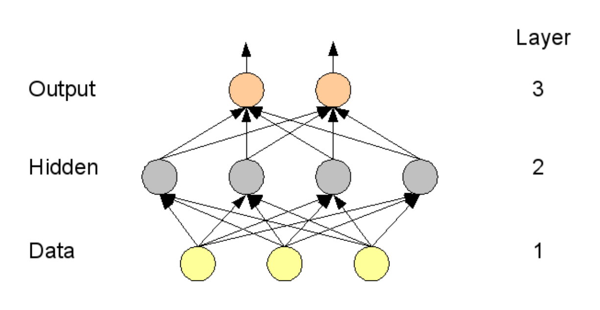
Training the network consists of clamping the data neurons at the data and updating the parameters (the weights and biases) in the direction of the gradient. The derivatives can be computed as follows:

$ \begin{aligned} \frac{\partial E}{\partial w_{ik}^{l-1}} &= \frac{\partial E}{\partial x_k^l} y_i^{l-1} \ \frac{\partial E}{\partial b_k^l} &= \frac{\partial E}{\partial x_k^l} \ \frac{\partial E}{\partial x_k^l} &= \frac{\partial E}{\partial y_k^l} \frac{\partial y_k^l}{\partial x_k^l} \ \frac{\partial E}{\partial y_k^l} &= \begin{cases} \frac{\partial E}{\partial y_k^L} & \text{if } l = L \ \sum_{i=1}^{N_{l+1}} \frac{\partial E}{\partial x_i^{l+1}} w_{ki}^l & \text{otherwise} \end{cases}. \end{aligned} $

$\frac{\partial E}{\partial y_k^L}$ is assumed to be readily computable and from this all the other derivatives can be computed, working down from the top layer. This is called the backpropagation algorithm.

Appendix C

Labeler instruction sheet

Section Summary: Labelers should include an image only if they would naturally describe its main object with the given category name, prioritizing the exclusion of mismatches over accidentally leaving out good fits. Reject images with multiple equally prominent objects, line drawings or cartoons, though photorealistic drawings are acceptable, and avoid dismissing them due to unusual viewpoints, partial occlusions, or busy or plain backgrounds. Duplicates can be included without worry since they will be removed later, and for categories with multiple meanings, stick to the primary one if unsure.

Criteria for deciding whether to include an image

1. The main test is: Would you be quite likely to say the category name if asked to give a single basic category to describe the main object in the image?

2. It's worse to include one that shouldn't be included than to exclude one. False positives are worse than false negatives.

3. If there is more than one object that is roughly equally prominent, reject even if they are all of the right class.

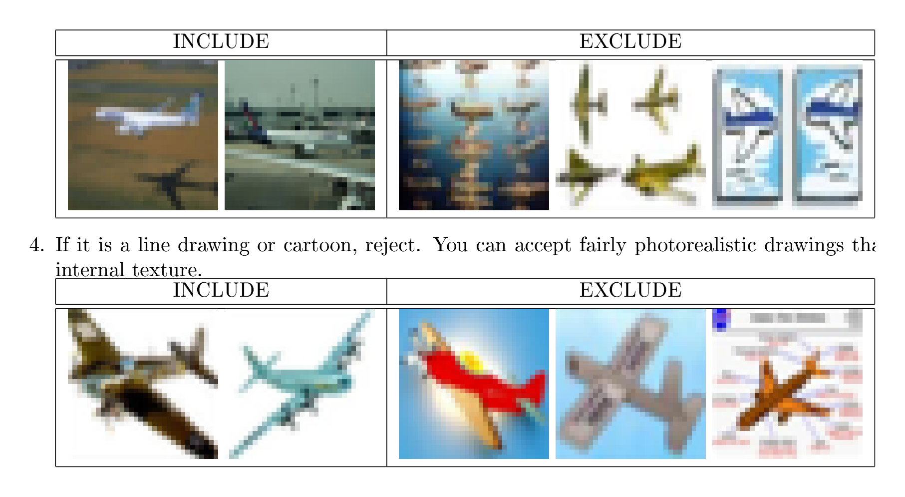
4. If it is a line drawing or cartoon, reject. You can accept fairly photorealistic drawings that have internal texture.

5. Do not reject just because the viewpoint is unusual or the object is partially occluded (provided you think you might have assigned the right label without priming). We want ones with unusual viewpoints.

6. Do not reject just because the background is cluttered. We want some cluttered backgrounds. But also, do not reject just because the background is uniform.

7. Do not worry too much about accepting duplicates or near duplicates. If you are pretty sure it's a duplicate, reject it. But we will eliminate any remaining duplicates later, so including duplicates is not a bad error.

8. If a category has two meanings (like mouse), only include the main meaning. If there is doubt about what this is, then ask.

Appendix D

CIFAR-100 class structure

Section Summary: The CIFAR-100 dataset organizes its 100 image categories into 20 broader groups called superclasses, with each superclass containing exactly five related classes. For instance, superclasses cover topics like aquatic mammals, flowers, household furniture, insects, and vehicles, ranging from natural elements like trees and animals to man-made items like food containers and electrical devices. When class names are plural, such as "bottles" or "apples," the dataset allows images showing multiple instances of those items.

Following is the class and superclass structure of the CIFAR-100 dataset. Each superclass contains five classes. Where the name of the class is plural, the labelers were instructed not to reject images in which multiple instances of the object appear.

1. aquatic mammals

   • beaver
   • dolphin
   • otter
   • seal
   • whale

2. fish

   • flatfish
   • ordinary fish (excluding trout and flatfish and salmon)
   • ray
   • shark
   • trout

3. flowers

   • orchids
   • poppies
   • rose
   • sunflowers
   • tulips

4. food containers

   • bottles
   • bowls
   • cans
   • cups, mugs, glasses
   • plates

5. fruit and vegetables

   • apples
   • mushrooms
   • oranges
   • pears
   • sweet peppers

6. household electrical devices

   • clock
   • computer keyboard
   • lamp
   • telephone
   • television

7. household furniture

   • bed
   • chair
   • couch
   • table
   • wardrobe

8. insects

   • bee
   • beetle
   • butterfly
   • caterpillar
   • cockroach

9. large carnivores

   • bear
   • leopard
   • lion
   • tiger
   • wolf

10. large man-made outdoor things

    • bridge
    • castle
    • house
    • road
    • skyscraper

11. large natural outdoor scenes

    • cloud
    • forest
    • mountain
    • plain
    • sea

12. large omnivores/herbivores

    • camel
    • cattle
    • chimpanzee
    • elephant
    • kangaroo

13. mid-size mammals

    • fox
    • porcupine
    • possum
    • raccoon
    • skunk

14. non-insect invertebrates

    • crab
    • lobster
    • snail
    • spider
    • worm

15. people

    • baby
    • boy
    • girl
    • man
    • woman

16. reptiles

    • crocodile
    • dinosaur
    • lizard
    • snake
    • turtle

17. small mammals

    • hamster
    • mouse
    • rabbit
    • shrew
    • squirrel

18. trees

    • maple
    • oak
    • palm
    • pine
    • willow

19. vehicles 1

    • bicycle
    • bus
    • motorcycle
    • pickup truck
    • train

20. vehicles 2

    • lawn-mower
    • rocket
    • streetcar
    • tank
    • tractor

Bibliography

Section Summary: This bibliography lists various academic papers, personal communications, and resources primarily related to artificial intelligence, neural networks, and machine learning techniques for tasks like image recognition and data processing. Key entries include works by researchers such as Geoffrey Hinton on training deep networks and reducing data dimensions, as well as studies on object recognition and lexical databases like WordNet, which is a tool for understanding English words and is accessible online. These sources span from the 1980s to 2009, providing foundational insights into unsupervised learning and computational models inspired by the brain.

[1] Bell, A. J., Sejnowski, T. J., 1997, The "independent components" of natural scenes are edge filters

[2] Bengio, Y., Lamblin, P., Popovici, D., Larochelle, H., 2006, Greedy Layer-Wise Training of Deep Networks

[3] Fergus, R., personal communication

[4] Freund, Y., Haussler, D., 1992, Unsupervised learning of distributions on binary vectors using two layer networks

[5] Hinton, G. E., 2002, Training Products of Experts by Minimizing Contrastive Divergence

[6] Hinton, G. E., Salakhutdinov, R. R., 2006, Reducing the dimensionality of data with neural networks

[7] Le Roux, N., 2009, personal communication

[8] Miller, G. A., 1995, WordNet: a lexical database for English

[9] Salakhutdinov, R., Murray, I., 2008, On the Quantitative Analysis of Deep Belief Networks

[10] Serre, T., Wolf, L., Bileschi, S., Riesenhuber, M., Poggio, T., 2007, Robust Object Recognition with Cortex-Like Mechanisms

[11] Smolensky, P., 1986, Information processing in dynamical systems: Foundations of harmony theory

[12] Teh, Y., Hinton, G. E., 2001, Rate-coded Restricted Boltzmann Machines for Face Recognition

[13] Tieleman, T., 2008, Training Restricted Boltzmann Machines using Approximations to the Likelihood Gradient

[14] Torralba, A., Fergus, R., Freeman, W. T., 2008, 80 million tiny images: a large dataset for non-parametric object and scene recognition

[15] WordNet can be found at http://wordnet.princeton.edu/